Efficient Aggregation of Multiple Classes of Information in Wireless Sensor Networks

Abstract
:
1. Introduction
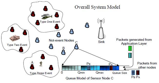
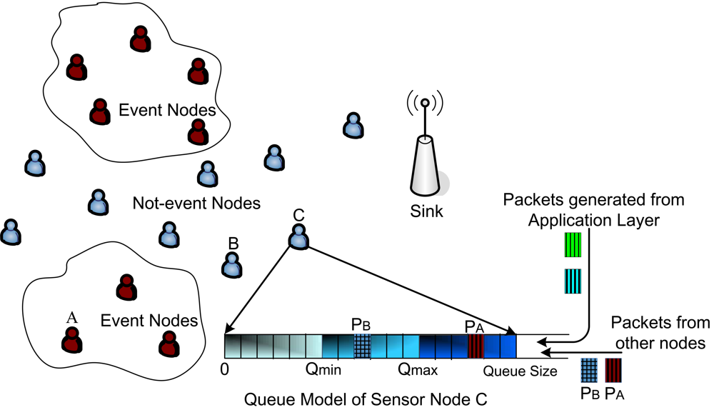
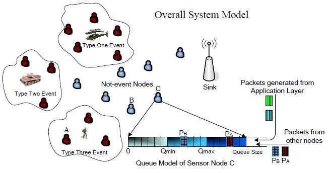
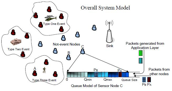
- In a WSN, packets with information of the desired event (Event packets), such as fires in the forest, are more important and urgent than those without event information (Non-Event packets). (Note that Non-Event packets are inevitable since sensor nodes need to contact with the sink periodically to notify that they are alive.) Therefore, in PCC we distinguish them with different priority thereby providing different throughput and dropping probability.
- When congestion occurs, packets from nodes far from the sink have a smaller chance to reach the destination than those from the nodes close to the sink [6]. Without any control, the WSN can only collect the information from the nodes near the sinks. Therefore, in PCC, we assign packets an index to store the probability of a packet successfully reaching any node along its path to the sink. Then PCC can dynamically adjust its dropping probability during congestion, to guarantee fairness for all nodes and coverage fidelity of the whole network.
- In a large WSN, wireless link quality changes according to multiple factors, such as obstacles between transmitter and receiver, multiple-path transmissions, and interference among neighbor links. In PCC, we consider the influence of link quality as an important parameter to indicate network resource utilization and the successful probability of transmissions.
- We make use of cumulative survival probability of a packet reaching a node along its path to the sink and the priority of different event information to design a mechanism to efficiently and fairly collect different categories of information in a single WSN, called Pricing System.
2. Priority-based Coverage-aware Congestion Control (PCC)
2.1. System Model and Design Considerations
- High Event Packets Throughput: In a WSN with both Event and Non-Event packets, it is important to ensure that Event packet throughput is high. In addition, since Event packet generation rate is normally higher than that of Non-Event packets, congestion may occur when events are detected by different sensor nodes simultaneously. Therefore, our mechanism should first guarantee high Event packet throughput when nodes are congested, to make sure that emergency information, like fire in the forest, is reported to the sink correctly and in a timely manner. We set up two thresholds in the sensor node queue to drop Event and Non-Event packets to give the former higher priority. To the best of our knowledge, few papers differentiate Event and Non-Event packets in WSNs with the exception of Event-to-Sink Reliable Transport (ESRT) [7]. Note that our work is different from ESRT, which is implemented in the transport layer and is an end-to-end congestion control method. PCC, on the other hand, is distributed and is based on network layer queue scheduling and MAC layer information feedback, as will be discussed in the following sections.
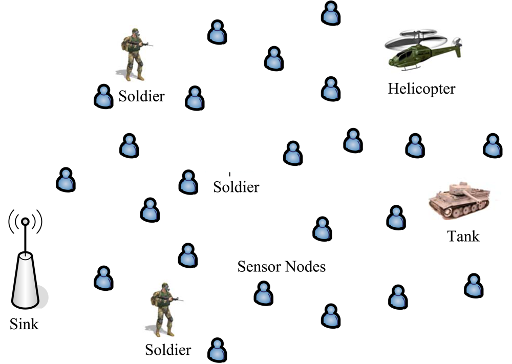
- Coverage Fidelity: As we explained in Section 1., packet throughput from a specific sensor node drastically decreases when packets traverse multiple hops to the sink. Therefore, packets generated by nodes nearby the sink have much higher probability of reaching the sink than those generated by nodes far away from the sinks. This leads to a spatial bias in the information collected in a multihop WSN. However, it is crucial to achieve coverage fidelity in a WSN because each monitoring area is usually equally important or remote areas are even more important since they are more difficult to be monitored by direct methods. Unlike other proposed methods, we consider the fairness among different areas at the application layer. Our proposed mechanism ensures that the sink receives equal number of packets with the same priority from all the sensor nodes in the sensor network. In IFRC [8], authors describe MAC layer fairness. However, MAC layer fairness does not ensure application layer fairness since the sink is biased to receive packets from nodes that are near it.
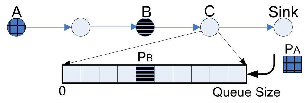
- Flexible Queue Scheduler: Most queue schedulers drop packets from the tail rather than any position in the queue. But tail-dropping does not work well in our new scheme. For instance, if the queue in a sensor node is near fully occupied and dominated with Non-Event packets, when an Event packet arrives, it is better to drop Non-Event packets because Event packets are more important. To address Coverage Fidelity, we can consider the scenario in Figure 3, where node B is closer to node C than node A, and the sink is at the rightmost end. If node A generates packet PA and node B generates packet PB simultaneously, PB will normally arrive at node C earlier. When PA arrives at node C whose queue is highly utilized, PA may be dropped while PB remains in the queue. This results in unfairness to different sensors. To mitigate this our proposed method checks the status of all packets in the queue and selectively drops packets according to an optimization algorithm, which will be introduced in the next section. With the help of a list of pointers to packets in the queue, it is feasible to drop intermediate packets with much lower complexity than expected.
- Resource Efficiency: Another important concern in a WSN is resource efficiency since sensor nodes usually have limited power and channel bandwidth [9, 10]. In a WSN, packets from sensors far from the sink normally consume more network resource than those from nodes nearby the sink. In our proposed method, we give preference to maintain packets from remote nodes since those packets have consumed more network resource and have lower probability to reach the sink when the intermediate relaying node experiences severe congestion. Therefore, when the same information is collected from different sensors in the network, our mechanism can efficiently utilize network resources by reducing the average number of point-to-point transmissions.
- MAC/PHY Link Quality: In a multihop WSN, the interference among neighboring links can severely reduce the transmission opportunities in MAC layer. In addition, in a WSN, wireless link qualities, such as noise and channel fading, are quite distinct according to locations, obstacles, etc. The link condition at MAC/PHY layer can also influence the success probabilities that packets reach the sink. In respect to resource efficiency, packets traveling through low quality links consume higher system resource since they require more re-transmission due to MAC collisions or more transmission time due to lower PHY layer transmission rate. Therefore, our mechanism will give packets traveling though poor quality links from remote nodes higher probability to reach the sink.
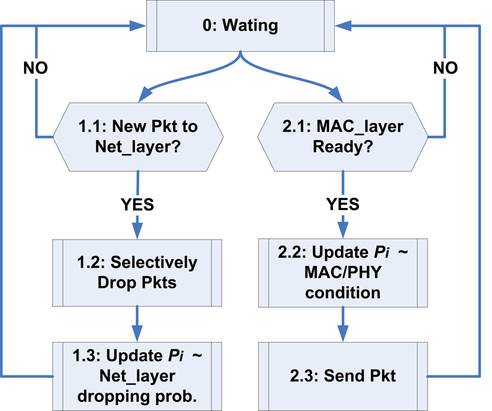
2.2. Protocol and Algorithm Design of PCC
Queue Handler
- 0 ≤ N ≤ Qmin: buffer all incoming packets.
- Qmin < N < Qmax: begin dropping Non-Event packets while keeping all Event packets. The dropping rate is selected such that the average number of Non-Event packets NN̄ = FN(N).
- Qmax ≤ N ≤ Q: drop all Non-Event packets and begin to drop some Event packets. The dropping rate is selected such that the average number of Event packets NĒ = FE(N).
| Algorithm 1 Optimization Algorithm | |
| Input: P⃗, F(N) | |
| Output: K | |
| 1: | Initial K ⇐ [0] |
| 2: | while TRUE do |
| 3: | for i = 1 to NP do |
| 4: | |
| 5: | end for |
| 6: | counter ⇐ 0 |
| 7: | for i = 1 to NP do |
| 8: | if ki > 1 then |
| 9: | ki ⇐ 1 |
| 10: | counter ⇐ counter + 1 |
| 11: | P⃗ ⇐ P⃗\Pi |
| 12: | end if |
| 13: | end for |
| 14: | if counter = 0 then |
| 15: | return K; |
| 16: | else |
| 17: | F(N) ⇐ F(N) − counter |
| 18: | end if |
| 19: | end while |
Link Quality Measurement
Discussions
2.3. Evaluation and Comparison
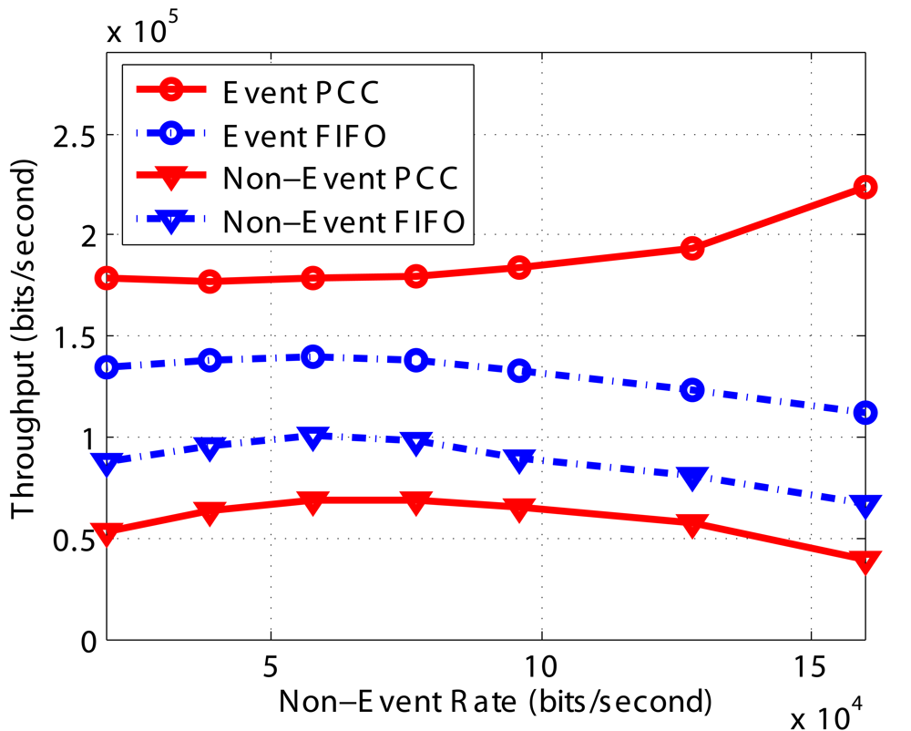
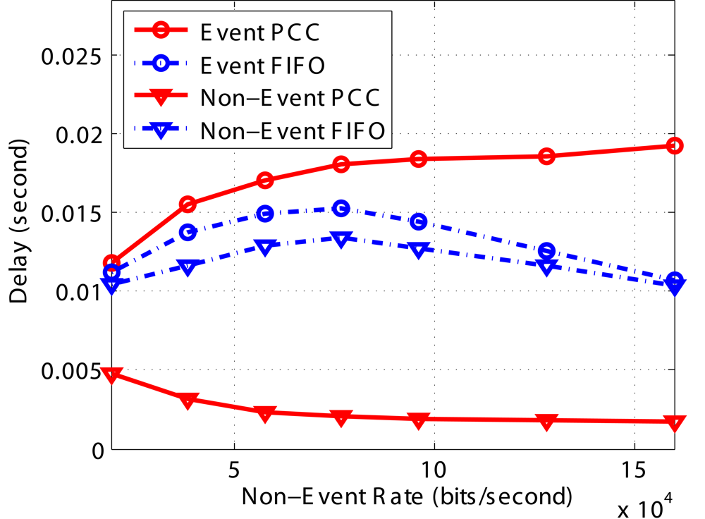
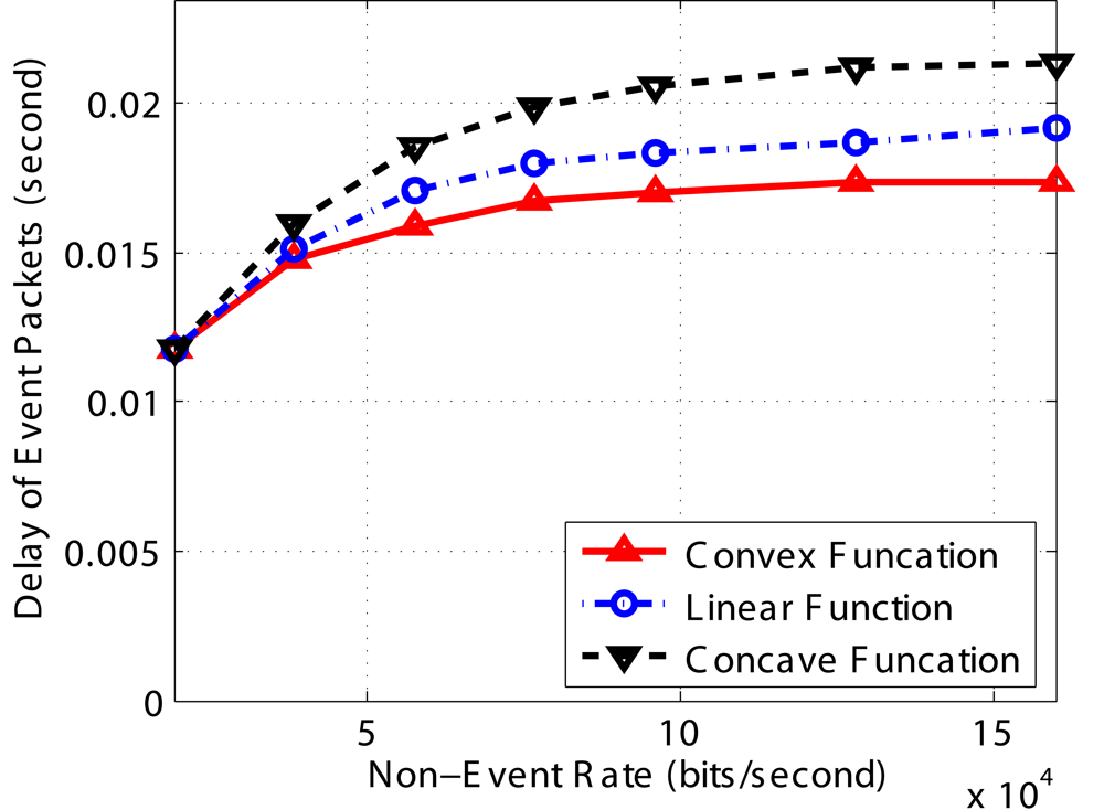
Throughput and Delay
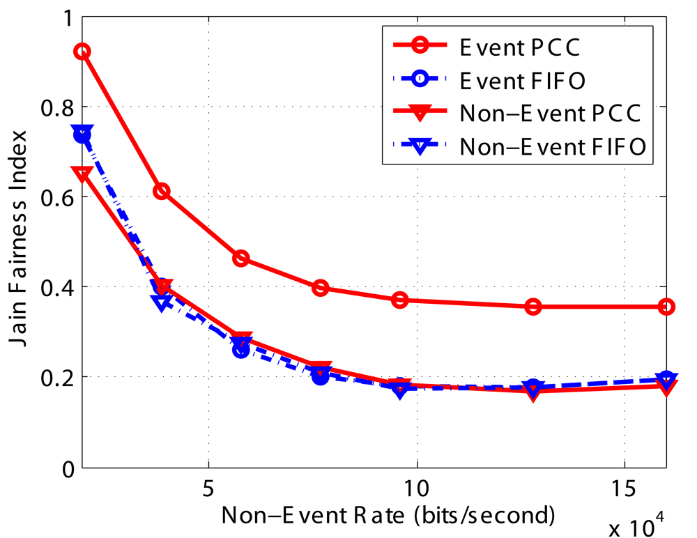
Coverage Fidelity
FE(N) and FN(N)
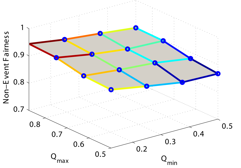
Qmin and Qmax
3. A Generalized Approach for Multiple Event Types
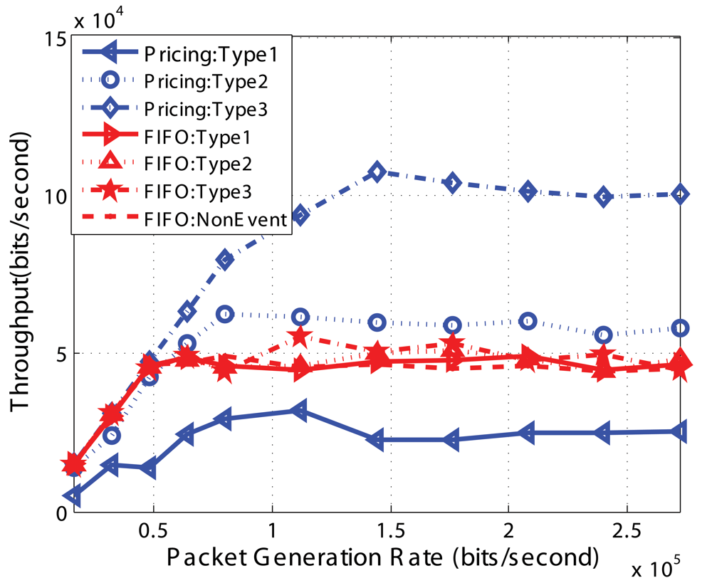
- The sink acts as the information consumer and sets a price that it is willing to pay for each different types of Event packets. Higher prices indicates the sink prefers the sensor network to collect this corresponding category of Event packet at the cost of more transmission resource. The ratio of different prices determines the balance between the priority and coverage. If all prices are equal, the Pricing system degrades to PCC. If one of the prices is ∞, the sink is willing to only accept the corresponding category of Event packets and consequently the wireless sensor network would block all other types of Event packets.
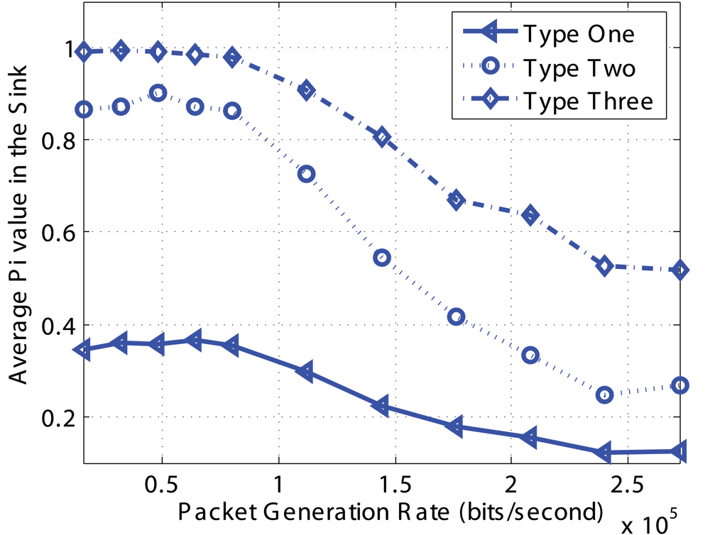
- The sensors operate as the information providers and when congested selectively drop packets according to the value that the sink places on the information in each packet (determined by the price set by the sink). When the buffer utilization is high, the sensor tends to keep packets with the lower accumulated survival probability Pi and higher price. The detailed algorithm is introduced in Section 3.1..
- The prices can dynamically vary according to the changes in the physical environment and the network condition. When the sink modifies the prices, the new prices are broadcast to the entire network and each sensor node uses the new prices to adjust the dropping policy during congestion.
3.1. Protocol and Algorithm
Task 1
Task 2
- 0 ≤ N ≤ Qmin: Keep all packets since the utilization of the buffer is low.
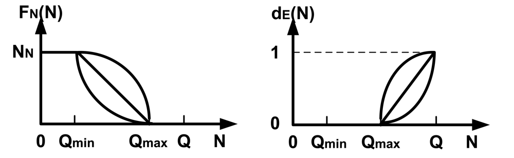
- Qmin ≤ N ≤ Qmax: Keep all types of Event packets and begin to drop Non-Event packets according to the function FN(N) shown in left part of Figure 5. The optimization problems becomessuch thatwhere R is the price of Non-Event packets, and K⃗N = [k1, k2, …, kNN] is the accepting probability, which is the decision variable. In the optimization algorithm, we would like the ratio of different type of price to be equal to the ratio of the cumulative survival probability of different types of packets as much as possible. The ideal case is when the Jain's Fairness Index equals 1, which is achieved when R1 : R2 : … : RM = P1k1 : P2k2 : … : PMkM. In other words, we ensure that Event packets for which the sink is willing to pay a higher price has higher accumulated survival probability (Piki) and the ratio of the cumulative survival probability follows the ratio of the prices. If two classes of packets traverse through similar network conditions, the ratio of throughput of these two types of packets should be similar to the ratio of the prices. Note that network condition includes both network link quality and the probability of being dropped in a node along the path to the sink. If the prices of two classes of packets are the same, we would like the probability of packets received at the sink to be the same. If all the prices are equal, the optimization problem becomes the same as Section 2.. Since all Non-Event packets have the same price and we selectively drop Non-Event packets, Equation 14 becomesNote that if R = 0, then ki = 0.
- Qmax ≤ N ≤ Q: After dropping all Non-Event packets, begin dropping Event packets since the buffer is highly utilized. The dropping strategy follows the optimization problem given by,such thatwhere Rj is the price of packet j, and K⃗E = [k1, k2, …, kNE] is the accepting probability, which is the decision variable. The meaning of the optimization is the same as explained in last paragraph. FE(N) = N + 1 − dE(N) and the dE(N) function are shown in the right part of Figure 5. Note that, if Rj = 0, then kj = 0.
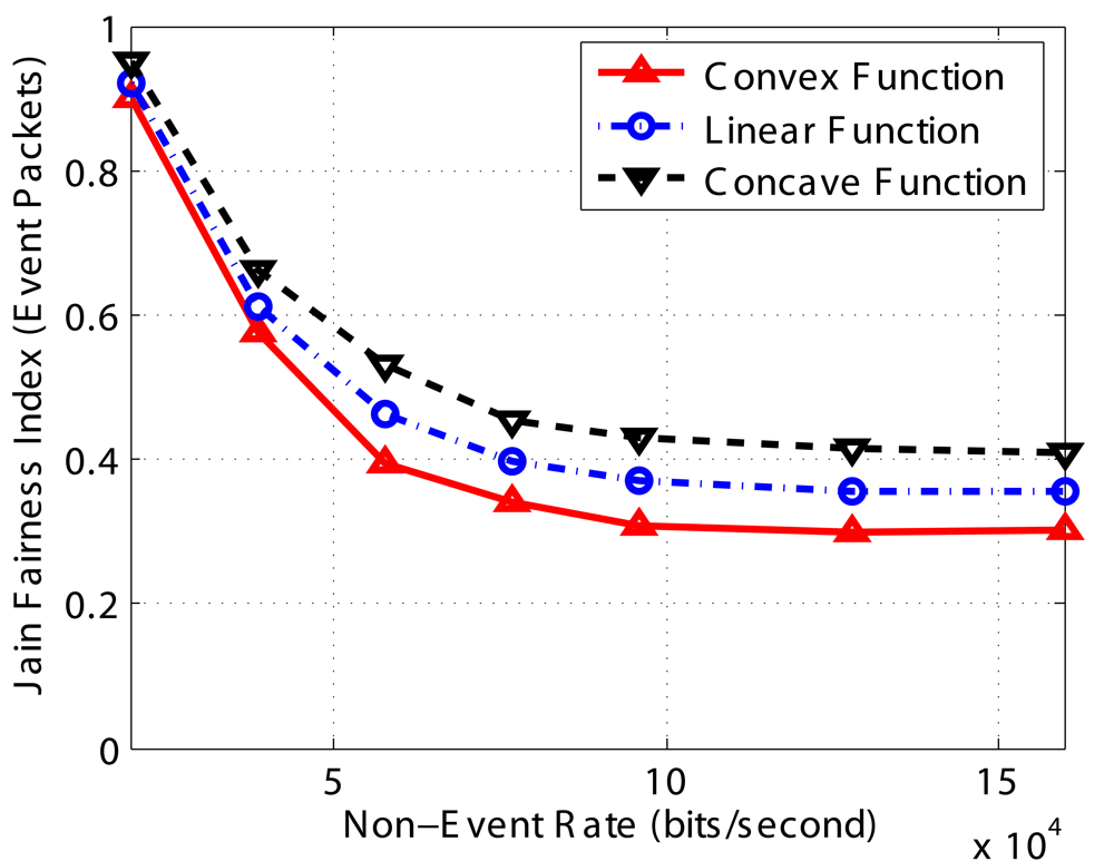
3.2. Simulations
4. Related Work
5. Conclusion
Acknowledgments
References and Notes
- Paek, J.; Chintalapudi, K.; Govindan, R.; Caffrey, J.; Masri, S. A Wireless Sensor Network for Structural Health Monitoring: Performance and experience. Proceedings of the 2nd IEEE Workshop on Embedded Networked Sensors, Washington, DC, USA; 2005. [Google Scholar]
- Rahimi, M.; Baer, R.; Warrior, J.; Estrin, D.; Srivastava, M.B. In Situ Image Sensing and Interpretation in Wireless Sensor Networks. Proceedings of the 3rd ACM Conference on Embedded Networked Sensor Systems (SenSys), San Diego, CA, USA; 2005. [Google Scholar]
- Qiu, X.; Ghosal, D.; Mukherjee, B.; Yick, J.; Li, D. Priority-Based Coverage-Aware Congestion Control for Multihop Sensor Networks. Proceedings of the 28th International Conference on Distributed Computing Systems Workshops, Beijing, China; 2008. [Google Scholar]
- Wikipedia. http://en.wikipedia.org/wiki/Motes (accessed in May, 2009).
- Dutta, P.; Taneja, J.; Jeong, J.; Jiang, X.; Culler, D. A Building Block Approach to Sensornet Systems. Proceedings of the Sixth ACM Conference on Embedded Networked Sensor Systems (SenSys), Raleigh, NC, USA; 2008. [Google Scholar]
- Cheng, X.; Mohapatra, P.; Lee, S.; Banerjee, S. Performance Evaluation of Video Streaming in Multihop Wireless Mesh Networks. Proceedings of the 18th International Workshop on Network and Operating Systems Support for Digital Audio and Video, Braunschweig, Braunschweig, Germany; 2008. [Google Scholar]
- Sankarasubramaniam, Y.; Akan, O.B.; Akyilidiz, I.F. ESRT: Event-to-Sink Reliable Transport in Wireless Sensor Networks. Proceedings of the 4th ACM International Symposium on Mobile Ad hoc Networking & Computing (MobiHoc), New York, NY, USA; 2003. [Google Scholar]
- Rangwala, S.; Gummadi, R.; Govindan, R.; Psounis, K. Interference-Aware Fair Rate Control in Wireless Sensor Networks. Proceedings of the Conference on Applications, Technologies, Architectures, and Protocols for Computer Communications, Pisa, Italy; 2006. [Google Scholar]
- Akyildiz, I.F.; Su, W.; Sankarasubramaniam, Y.; Cayirci, E. A Survey on Sensor Networks. IEEE Commun. Mag. 2002, 8, 142–114. [Google Scholar]
- Yick, J. Advanced Services in Wireless Sensor Networks. Ph.D Thesis, University of California, Davis, CA, USA, 2006. [Google Scholar]
- Jain, R. The Art of computer systems Performance Analysis, 1st ed.; Wiley: New York, NY, USA, 1991. [Google Scholar]
- Mitchell, M.T. Machine Learning, 1st ed.; McGraw Hill: New York, NY, USA, 1997. [Google Scholar]
- Floyd, S.; Jacobson, V. Random Early Detection Gateways for Congestion Avoidance. IEEE ACM Trans. Netw. 1993, 1, 397–413. [Google Scholar]
- Perkins, C.; Royer, E. Ad-hoc On-Demand Distance Vector Routing. Proceedings of the 2nd IEEE Workshop on Mobile Computing Systems and Applications, New Orleans, LA, USA; 1999. [Google Scholar]
- Wan, C.-Y.; Eisenman, S.B.; Campbell, A.T. CODA: Congestion Detection and Avoidance in Sensor Networks. Proceedings of the First ACM Conference on Embedded Networked Sensor Systems (SenSys), Los Angeles, CA, USA; 2003. [Google Scholar]
- Iyer, Y.G.; Gandham, S.; Venkatesan, S. STCP: A Generic Transport Layer Protocol for Wireless Sensor Networks. Proceedings of 14th International Conference on Computer Communication and Networks (ICCCN), San Diego, USA; 2005. [Google Scholar]
- Zhou, Y.; Lyu, M.R. PORT: A Price-Oriented Reliable Transport Protocol for Wireless Sensor Networks. Proceedings of IEEE Symposium on Software Reliability Engineering (ISSRE), Chicago, IL, USA; 2005. [Google Scholar]
- Wang, C.; Sohraby, K.; Li, B. SenTCP: A Hop-by-Hop Congestion Control Protocol for Wireless Sensor Networks. Proceedings of IEEE INFOCOM, Miami, FL, USA; 2005. [Google Scholar]
- Sheu, J.-P.; Hu, W.-K. Hybrid Congestion Control Protocol in Wireless Sensor Networks. Proceedings of IEEE Vehicular Technology Conference (VTC), Marina Bay, Singapore; 2008. [Google Scholar]
- Paek, J.; Govindan, R. RCRT: Rate-Controlled Reliable Transport for Wireless Sensor Networks. Proceedings of the 5th ACM Conference on Embedded Networked Sensor Systems (SenSys), Sydney, Australia; 2007. [Google Scholar]
- Liu, Y.; Liu, Y.; Pu, J.; Xiong, Z. A Robust Routing Algorithm with Fair Congestion Control in Wireless Sensor Network. Proceedings of 17th International Conference on Computer Communications and Networks (ICCCN), St. Thomas, U.S. Virgin Islands, USA; 2008. [Google Scholar]
- Teo, J.-Y.; Ha, Y.; Tham, C.-K. Interference-Minimized Multipath Routing with Congestion Control in Wireless Sensor Network for High-Rate Streaming. IEEE Trans. Mobile Comput. 2008, 7, 1124–1137. [Google Scholar]
- Chen, J.; Zhou, M.; Li, D.; Sun, T. A Priority Based Dynamic Adaptive Routing Protocol for Wireless Sensor Networks. Proceedings the Workshop on Intelligent Networks and Intelligent Systems, Beijing, China; 2008. [Google Scholar]
- Hsu, Y.-P.; Feng, K.-T. Cross-layer Routing for Congestion Control in Wireless Sensor Networks. Proceedings of 2008 IEEE Radio and Wireless Symposium, Orlando, FL, USA; 2008. [Google Scholar]
- Society, I.C. IEEE Standard 802.11: Wireless LAN Medium Access Control (MAC) and Physical Layer (PHY) Specifications.; IEEE: Piscataway, NJ, USA, 1997. [Google Scholar]
- Ee, C.T.; Bajcsy, R. Congestion Control and Fairness for Many-to-One Routing in Sensor Networks. Proceedings of the Second ACM Conference on Embedded Networked Sensor Systems (SenSys), Baltimore, MD, USA; 2004. [Google Scholar]
- Hull, B.; Jamieson, K.; Balakrishnan, H. Mitigating Congestion in Wireless Sensor Networks. Proceedings of the Second ACM Conference on Embedded Networked Sensor Systems (SenSys), Baltimore, MD, USA; 2004. [Google Scholar]
- Wang, C.; Sohraby, K.; Lawrence, V.; Li, B.; Hu, Y. Priority-based Congestion Control in Wireless Sensor Networks. Proceedings of IEEE International Conference on Sensor Networks, Ubiquitous, and Trustworthy Computing, Washington, DC, USA; 2006. [Google Scholar]
- Li, Z.; Liu, P.X. Priority-based Congestion Control in Multi-path and Multi-hop Wireless Sensor Networks. Proceedings of IEEE Conference on Robotics and Biomimetics, Sanya, China; 2007. [Google Scholar]
- Yaghmaee, M.H.; Adjeroh, D. A New Priority based Congestion Control Protocol for Wireless Multimedia Sensor Networks. Proceedings of International Symposium on a World of Wireless, Mobile and Multimedia Networks (WoWMoM), Washington, DC, USA; 2008. [Google Scholar]
- Monowar, M.M.; Rahman, M.O.; Hong, C.S. Multipath Congestion Control for Heterogeneous Traffic in Wireless Sensor Network. Proceedings of 10th International Conference on Advanced Communication Technology (ICACT), Gangwon-Do, Korea; 2008. [Google Scholar]


| Node 1 | Node 2 | Node 3 | Jain's Fairness Index | |
|---|---|---|---|---|
| Event PCC | 139 | 130 | 135 | 0.99925 |
| Event FIFO | 297 | 77 | 20 | 0.54735 |
| Non-Event PCC | 149 | 125 | 124 | 0.99247 |
| Non-Event FIFO | 292 | 60 | 23 | 0.52437 |
© 2009 by the authors; licensee Molecular Diversity Preservation International, Basel, Switzerland. This article is an open access article distributed under the terms and conditions of the Creative Commons Attribution license (http://creativecommons.org/licenses/by/3.0/).
Share and Cite
Qiu, X.; Liu, H.; Li, D.; Yick, J.; Ghosal, D.; Mukherjee, B. Efficient Aggregation of Multiple Classes of Information in Wireless Sensor Networks. Sensors 2009, 9, 8083-8108. https://doi.org/10.3390/s91008083
Qiu X, Liu H, Li D, Yick J, Ghosal D, Mukherjee B. Efficient Aggregation of Multiple Classes of Information in Wireless Sensor Networks. Sensors. 2009; 9(10):8083-8108. https://doi.org/10.3390/s91008083
Chicago/Turabian StyleQiu, Xiaoling, Haiping Liu, Deshi Li, Jennifer Yick, Dipak Ghosal, and Biswanath Mukherjee. 2009. "Efficient Aggregation of Multiple Classes of Information in Wireless Sensor Networks" Sensors 9, no. 10: 8083-8108. https://doi.org/10.3390/s91008083