1. Introduction
The failure of several major dams causing great destruction and high death tolls has led to a systematic monitoring of major dams and reservoirs in order to ensure their structural integrity, the prevention of major damage, and especially, the safety of the public. Driven by the development of measuring and analysis techniques, the goal of geodetic deformation analysis nowadays is to proceed from a merely phenomenological description of the deformation of an object to the analysis of the process which caused the deformation [
1]. Analysis of deformations of any type of a deformable body includes geometrical analysis and physical interpretation. Geometrical analysis describes the change in shape and dimensions of the monitored object. The ultimate goal of the geometrical analysis is to determine in whole deformable object the displacements and strain fields in the space and domains. Physical interpretation is to establish the relationship between the causative factors (loads) and the deformations. This can be determined either by statistical method, which analyses the correlation between the observed deformations and loads [
2].
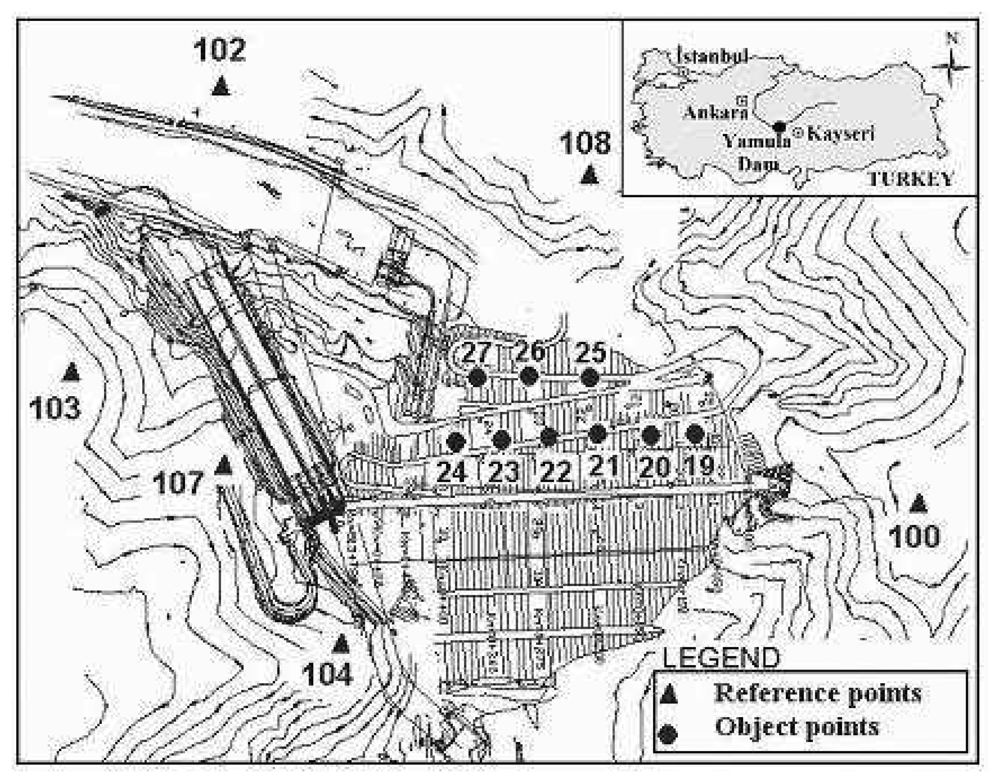
In this study, as an example, the effect of pressure of water on the dam settlement during the first filling of reservoir is shown, with geodetic monitoring results using statistical methods, which analyse the correlation between the observed deformations and loads. Thus, we analyze four geodetic records covering the first filling period, describe the subsidence of the body of a large size earth fill dam, called The Yamula, and try to investigate the effect of the increase of the reservoir level on the dam. The problem is, thus, how the rising water level of the reservoir effects the vertical deformations of the dam during the first filling period. A developed deformation model was used to answer this question. The dynamic model contains the calculation of a parameter of the rising reservoir level, which shows the geometric signature of the physical effect. Finally, the acceleration effect of rising level in large reservoirs on the dam deformations was investigated.
3. Dynamic analysis
The first filling period of a dam is the most dangerous and interesting period in a dam's life. At the reservoir filling stage two main effects must be considered: pressure of water and effect of wetting [
2,
3]. In this model, as an example, the effect of the water pressure on the dam settlement during the first filling of the reservoir is shown with the geodetic monitoring results. An attempt was made to correlate the dam settlement and with water level. For this, it was assumed that the relationship between water level and the dam settlement was linear. Using this approach, a new model “
x =
f (
t,
WL) “was developed. Here
WL represents reservoir level which is one of the causes of the vertical displacements affecting the point positions on the dam and is a dynamic variable. If
x =
f (
t,
WL) is expanded with a Taylor series to the first degree,
where Δ
WL and
t are the difference of reservoir water levels and period of time between the two periods; and
b is the water level parameters. The one-dimensional dynamic model consisting of position and water level can be written as below. In
Equation (3), the unknown movement parameters consist of position and water level (first derivative of position according to water level changes). The two unknown parameters can be calculated using the Kalman-Filter technique with two measurement periods. In the Kalman-Filter technique, the movement parameters at the present time are predicted with those of the preceding (
ti-1) period. Finally, the filtered (adjusted) parameters are computed, combining the predicted information and the measurements at the
ti period. To compute the movement parameters of the points with the Kalman-Filter technique, equations of position and water level can be written as below.
Equations (3) and
(4) can be represented in matrix form, as given in
or in a shorter form
where
Y̅i = predicted state (position, water level) vector at period
ti;
Yˆ
i-1 = state vector at period
ti-1;
Ti,i-1 = transition matrix and
I = unit matrix.
Equation (6) is the prediction equation, which is the basic equation of a Kalman-Filter;
w = constant violator acceleration vector and
N = the system noise vector.
w cannot be measured as a rule, so it can be taken as zero.
N is the last column of the
T matrix between periods
ti and
ti-1. The prediction equation and covariance matrix in
Equation (6) can be rewritten as
where
QYˆYˆ,i-1 =cofactor matrix of the state vector; and
Qww,
i-1 = cofactor matrix of the system noise at time
ti-1.
Qww,
i-1 can be predicted as follows.
The adjustment of the problem can be expressed in matrix form as
where
li,
v1,
i,
A, and
Yˆi = measurements in epoch
i, residuals, coefficients matrix, and state vector at time
ti, respectively. The functional and stochastic models for the Kalman-Filter technique combining
Equations (7) and
(10) can be written in matrix form as
The model is solved and the movement parameters and their cofactor matrix are computed. Thus, with the Kalman-Filter technique, the two unknown parameters can be computed with two measurement periods [
4-
11]
As mentioned above, the parameters of position and water level are included in this process. The results of a global test of the model are shown in
Tables 1 and
2, where,
a priori variance (s
0) was computed in a preliminary network adjustment.
A posteriori variance (m
0) was computed from the model.
. q is the
F-distribution value. According to [
12], if T<q, the global test is valid. As can be seen from
Tables 1 and
2, all global test values are smaller than the α-percentage point of the
F-distribution value (q) for a confidence level of α=0.05. Thus, the model can be viewed as accurate enough for this confidence level. That is, the global tests of the developed model are valid.
Because there is not any significant displacement in the x coordinates, these are not taken into consideration in this model. The movement parameters [vertical and horizontal displacement, (only y coordinate), water level] were computed using the dynamic method in one dimension and the results of the object points for the December 2003-November 2004, and December 2003-April 2005 are given in
Table 3 for vertical displacements, and
Table 4 for horizontal displacements. Because no significant settlement was determined, results of the object points for the periods of December 2003-March 2004 aren't given. Here, every parameter was divided by its standard deviation, and test values (T
z, T
bz, T
y, T
by) were computed. These values were compared with the t-distribution value (q
t) to evaluate whether they were significant or not [
13]. Where parameters have significantly changed, a (+) sign is shown; otherwise, a (−) sign is shown in decision column.
4. Discussion
Deformation analysis results of the dynamic model for object points located on the dam are shown in
Tables 3 and
4. These tables indicate that all object points except for 19, 20, and 27 on the dam showed significant movements. Results can be noted that displacements and water level effects are maximum at the middle of the dam.
The dynamic model contains a water level parameter, which shows the physical effect of the reservoir water level on the displacements of object points. The water level parameters have physical meanings. The sign of the water level parameter is significant to be able to interpret the effect of the reservoir water level on the settlements. When analyzing the sign and the magnitude of this parameter, the effect of water level on point settlements can be determined. If “the sign of the water level parameter in decision column is positive”, a rise in the reservoir level causes settlements. If “the sign of the water level parameter in decision column is negative”, there are no settlements. When examining the water level parameters, it can be seen from
Table 3 and
4 that the signs of the water level parameter in decision column except for 19, 20, and 27 are positive.
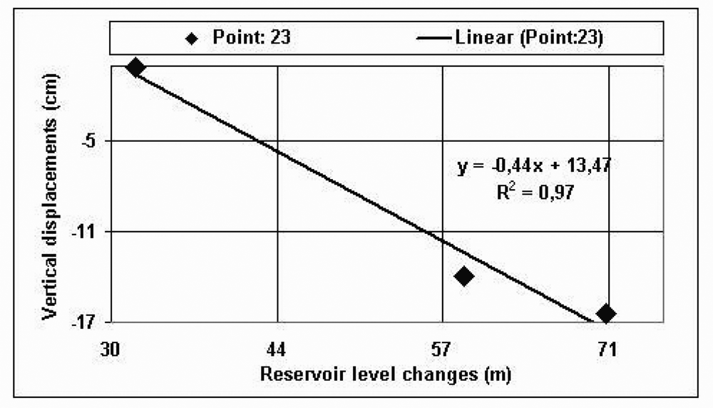
The dynamic model shows the relationship between the rise in reservoir water level and the observed structural deformation of the dam. This relationship had been assumed as linear. An attempt was made to correlate the vertical displacements of object points and water level. In order to verify this assumption, the squares of the correlation coefficients were computed in order to find the relationship between the reservoir level and the point displacements. A graphic (
Figure 2) was drawn for point 23 as an example. The graphic shows the relationship between the reservoir level and computed subsidence. The results of square of correlation coefficients for point 23 are given in
Table 5. Where, WL, z, and y are the water level changes, vertical displacements and horizontal displacements between the measurement epochs, respectively. R
2 in
Figure 2 is the square of correlation coefficient. R
2 gives the proportion of sample variety in dependent variable (displacements) that is explained by independent variable (the rise in the reservoir level). For point 23, R
2 means that 97% of the variability in the dependent variable is explained by the independent variable and 3% is unexplained. R
2 values for the moving points (21, 22, 23, 24, 25, and 26) are seen in
Table 5 and
6.
Table 6 shows results of square of correlation coefficients for moved points.
As shown in
Figure 2 and
Tables 5 and
6, there is an apparent linear relation between the dam settlement and the rise in the reservoir level. In addition, there was evidence of the rise in water level in the magnitude of the displacements.
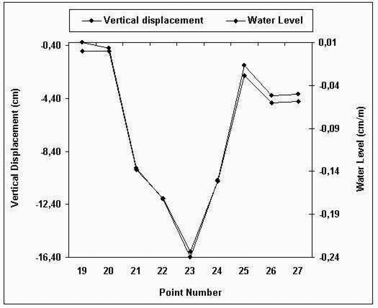
This situation can be seen in
Figure 3. In
Figure 3, the relationship between the water level parameter and displacements was established for the period of December 2003- April 2005 (data from
Table 3 for Period: December 2003- April 2005).
Relationships for all measurement periods are given in
Table 7. When examining relationships between displacements and water level parameters, it can be seen (
Figure 3 and
Table 7) that there is a strong harmony. This means that the rising water level increases the subsidence of all object points (except for 19, 20 and 27). That is, all object points (except for 19 and 29) were affected by the rise in water level during to first filling period.


