Improving Estimation Performance in Networked Control Systems Applying the Send-on-delta Transmission Method

Abstract

This paper is concerned with improving performance of a state estimation problem over a network in which a send-on-delta (SOD) transmission method is used. The SOD method requires that a sensor node transmit data to the estimator node only if its measurement value changes more than a given specified δ value. This method has been explored and applied by researchers because of its efficiency in the network bandwidth improvement. However, when this method is used, it is not ensured that the estimator node receives data from the sensor nodes regularly at every estimation period. Therefore, we propose a method to reduce estimation error in case of no sensor data reception. When the estimator node does not receive data from the sensor node, the sensor value is known to be in a (−δ_i,+δ_i) interval from the last transmitted sensor value. This implicit information has been used to improve estimation performance in previous studies. The main contribution of this paper is to propose an algorithm, where the sensor value interval is reduced to (−δ_i/2,+δ_i/2) in certain situations. Thus, the proposed algorithm improves the overall estimation performance without any changes in the send-on-delta algorithms of the sensor nodes. Through numerical simulations, we demonstrate the feasibility and the usefulness of the proposed method.

1. Introduction

Recently, interest in the study of networked control system (NCS) and sensor networks has increased widely due to its low cost, high flexibility, simple installation and maintenance [1]. In such systems, a center station has the task of receiving, processing and sending data to the slave nodes such as sensor nodes, actuator nodes, etc. over a serial network. It is easy to add or remove slave nodes in the network without changing the system structure much. Aside from the advantages as mentioned above, however, there are several problems affecting to the system such as bandwidth, network-induced delay, packet loss rate.

One of the most interesting problems is how to reduce network bandwidth when there are many nodes on the network. This can be achieved by reducing either data packet size or data packet transmission rate. In [2], an adjustable deadband was defined on each node to reduce network traffic. The node does not broadcast a new message if its signal is within the deadband. In [3], estimators were used at each sensor node instead. When the estimated value deviates from the actual output by more than a prespecified tolerance, the actual sensor data are transmitted. To overcome the limited network bandwidth, transmission data size reduction using a special encoder-decoder was considered in [4]. Another method for reduction of data transmission rate called send-on-delta (SOD) transmission was explored in [5-8]. This method requires that a sensor node transmit data to the estimator node only if its measurement value changes more than a given specified δ value. By adjusting the δ value at each sensor node, data transmission rate is reduced so that the network bandwidth is increased and can be used for other traffic.

The purpose of this paper is to extend our work on the modified Kalman filter employing a SOD transmission method [5], where the states are periodically estimated by the estimator node regardless of whether the sensor nodes transmit data or not. A challenging issue is how the estimator node determines the measurement value at a sensor node if it does not send data. If this problem is well solved, the estimation performance will be significantly improved. In this paper, we examine and evaluate the measurement output value as well as measurement noise arising when a sensor node does not transmit data. Then, a computed output with the new measurement value and new noise covariance is compensated to the system in order to reduce estimation error. Through simulations, we show that the proposed method gives better estimation performance than that of [5].

2. Sensor Output Evaluation

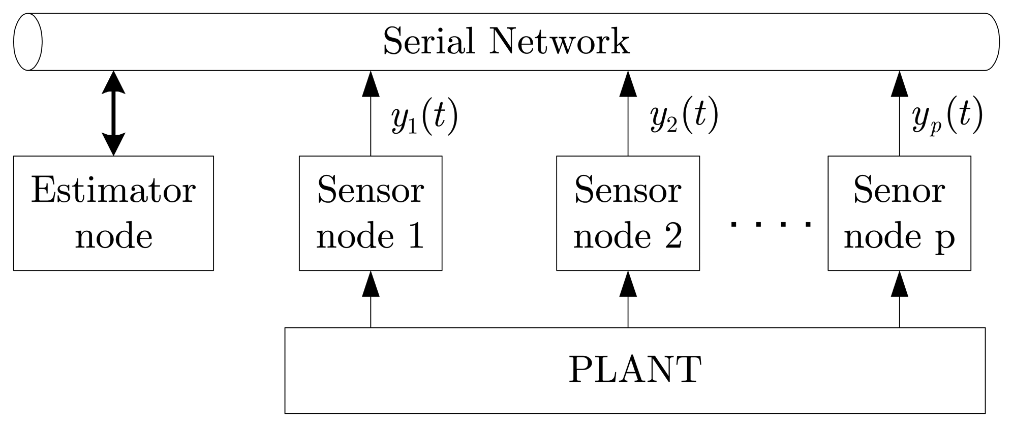
Consider a networked control system illustrated as in Figure 1, where the linear continuous-time system is described as:

$$\begin{array}{ll}\dot{x}(t)\hfill & =Ax(t)+Bu(t)+w(t)\hfill \\ y(t)\hfill & =Cx(t)+v(t)\hfill \end{array}$$

(1)

where x ∈ Rⁿ is the state of the plant, u is the deterministic input signal, y ∈ R^p is the measurement output which is sent to the estimator node by the sensor nodes. w(t) is the process noise with covariance Q, and v(t) is the measurement noise with covariance R. w(t) and v(t) are uncorrelated, zero mean white Gaussian random processes.

The following assumptions are made on the data transmission over network:

• Measurement outputs are s y_i(1 ≤ i ≤ p) are sampled at period T, but their data are only transmitted to the estimator node when the difference between the current value and the previously transmitted one is greater than δ_i.
• For simplicity in problem formulation, any transmission delay from the sensor nodes to the estimator node is ignored.

The estimator node estimates the states of the plant regularly at period T, regardless of whether or not any sensor data arrive. If the i-th sensor data do not arrive, the estimator node knows that the current value of i-th sensor output has not changed more than the range (−δ_i,+δ_i), compared with the last arriving one. This implicit information is used to estimate the current states in case i-th sensor data do not arrive.

Let the last received value of i-th sensor output be y_last,i, at time t_last,i. If there is no sensor data received for t > t_last,i, the estimator node considers that the measurement value of the i-th sensor output y_i(t) is still equal to y_last,i but the measurement noise is increased from v_i(t) to v_n,i(t) = v_i(t) + Δ_i(t,t_last,i), where Δ_i(t,t_last,i) is defined [5]:

$${\mathrm{\Delta }}_i(t,t_{\mathit{\text{last}},i})=y_{\mathit{\text{last}},i}-y_i(t),\left|{\mathrm{\Delta }}_i(t,t_{\mathit{\text{last}},i})\right|\le {\delta }_i$$

(2)

In [5], it was assumed that Δ_i(t,t_last,i) had a uniform distribution with zero mean and a variance ${\delta }_1^2/3$. However, this assumption is incorrect in some cases where that measurement noise R_(i,i) is smaller than ${\delta }_1^2$, where R_(i,i) is the (i,i)-th element of R. To illustrate this, assume that there is no measurement noise (i.e., R=0). Then 0 ≤ Δ_i(t,t_last,i) < δ_i if Cx(t) is increasing and − δ_i < Δ_i (t,t_last,i) ≤ 0 if Cx(t) is decreasing. In this case, a reasonable assumption is that the mean of Δ_i(t,t_last,i) is δ_i /2 if Cx(t) is increasing and − δi /2 if Cx(t) is decreasing. This trend is preserved as long as the measurement covariance R ≪ δ². When the measurement covariance is large, then Δ_i(t,t_last,i) in [5] is more likely affected by the zero-measurement noise v(t); thus zero mean assumption is a more valid assumption.

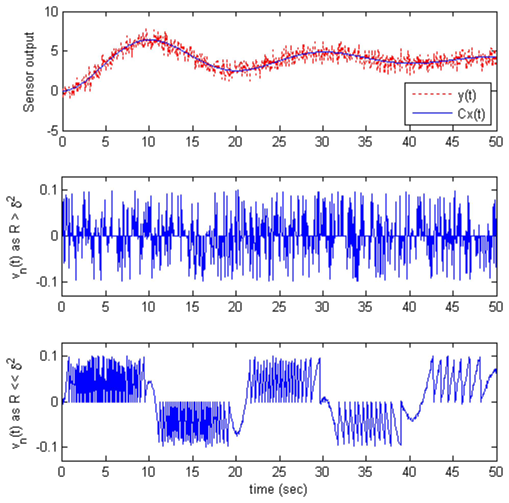
To demonstrate this argument, consider an example of the output response of an 2^nd order system with step input shown in Figure 2. The top graph is the output signal without noise Cx(t) and the measurement output y(t). In this example, y(t) is sampled by the send-on-delta scheme with δ = 0.1. The new measurement noise v_n(t) is shown in the middle and bottom graphs for two cases: R > δ² and R ≪ δ², respectively. Obviously, the waveform of v_n(t) is rather different in two cases: It is a uniform distribution with zero mean in the first case, but with non zero mean in the second case. For example, v_n(t) has a positive mean value in time range (0,10s) but a negative mean value in (10,20s).

Therefore, the assumption in [5] is only correct in the case R > δ². Furthermore, in realistic systems, measurement noise is normally small, while δ is set to a greater value to reduce data transmission rate. For some types of digital sensor such as encoders, measurement noise is even equal to zero. This means that the second case (non-zero mean case) happens more usually than the first case in the real applications. We propose an estimation algorithm which exploits this non-zero mean case in order to improve the estimation performance.

Now we compute the mean value and variance of v_n,i(t). Notice that the new measurement noise v_n,i(t) only exists when the estimator node does not receive data from the i-th sensor node at instant t. Otherwise, measurement noise is still v_i(t).

$$\begin{array}{l}+\text{If}{R}_{(i,i)}>{\delta }_i^2:\hfill \\ E\{v_{n,i}(t)\}=0\hfill \\ \mathit{\text{Var}}\{v_{n,i}(t)\}=R_{(i,i)}+{\delta }_i^2/3\hfill \end{array}$$

(3)

$$\begin{array}{l}+\text{If}{\mathit{\text{R}}}_{(i,i)}\le {\delta }_i^2:\hfill \\ E\left\{v_{n,i}\left(t\right)\right\}={\delta }_i/2(or-{\delta }_i/2)\hfill \\ \mathit{\text{Var}}\left\{v_{n,i}\left(t\right)\right\}=R_{(i,i)+}{\delta }_i^2/12\hfill \end{array}$$

(4)

We see that variance of v_n,i(t) in the second case (4) is smaller than in (3) which was used in [5].

3. State estimation with the SOD transmission method

In this section, we propose a method to adaptively use (3) or (4) in the modified Kalman filter for the state estimation problem. The main issue here is when we should use (4) instead of (3)? And if (4) is used, how then to determine when the mean value of v_n,i(t) is positive or negative?

Firstly, we compute the mean value of v_n,i(t) when (4) is used. Let two latest consecutive i-th sensor output values received at the estimator node be y_last−1,i, y_last,i at time t_last−1,i, t_last,i, respectively. Derivative of y_i at time t_last,i is approximately calculated as follows:

$$y_i^{\prime }(t_{\mathit{\text{last}},i})\approx \frac{{\widehat{y}}_{\mathit{\text{last}},i}-{\widehat{y}}_{\mathit{\text{last}}-1,i}}{t_{\mathit{\text{last}},i}-t_{\mathit{\text{last}}-1,i}}=\frac{{\widehat{y}}_{\mathit{\text{last}},i}-{\widehat{y}}_{\mathit{\text{last}}-1,i}}{k_{i}T}$$

(5)

where ŷ_last,i is the estimated value of y_i(t) at instant t_last,i, and k_i is number of sampling times. We use ŷ_last,i instead of y_last,i to reduce measurement noise effects. If the i-th sensor node does not send data at instant t > t_last,i, it is more likely that the output value y_i(t) will satisfy:

$$\begin{array}{l}{\widehat{y}}_{\mathit{\text{last}}-1,i}<{\widehat{y}}_{\mathit{\text{last}},i}<y_i(t)\hfill \\ \text{or}\hfill \\ y_i(t)<{\widehat{y}}_{\mathit{\text{last}},i}<{\widehat{y}}_{\mathit{\text{last}}-1,i}\hfill \end{array}$$

Therefore, mean value of the new measurement noise v_n,i(t) is computed:

$$E\{v_{n,i}(t)\}\triangleq \mathit{\text{sign}}(y_i^{\prime }(t_{\mathit{\text{last}},i}))*{\delta }_i/2$$

(6)

Once E{v_n,i(t)} is obtained in (6), to satisfy zero mean noise condition in the Kalman filter, we just add this value to the measurement value y_last,i.

Now we investigate the system response to determine when (3) or (4) is chosen to the filter. The basic principle is that if it is certain that y_i(t) is increasing or decreasing, we should use (4). And if it is not certain, we should use (3). This decision is made based on the absolute value of $y_i^{\prime }(t)$ as follows:

$$\mathit{\text{Selector}}=\{\begin{array}{c}(3),\text{if}|y_i^{\prime }(t_{\mathit{\text{last}},i})|\le {\mathit{\epsilon }}_i\hfill \\ (4),\text{otherwise}\hfill \end{array}$$

(7)

where ε_i > 0 is a sufficiently small threshold. If $\left|y_i^{\prime }(t_{\mathit{\text{last}},i})\right|$ is small, it is difficult to draw a meaningful conclusion about whether y_i(t) is increasing or decreasing, so in that case, we use (3). Otherwise, we could be fairly certain about whether y_i(t) is increasing or decreasing; in that case, we use (4). Some remarks about the parameter ε_i are warranted. If ε_i = ∞, (3) is always used in the filter as in [5]. Therefore, in case $R_{(i,i)}>{\delta }_i^2$, the proposed filter will become to the filter in [5] if setting ε_i = ∞. It is very flexible to switch the filter to [5] or to the the proposed filter so that estimation performance is improved in both case R > δ² and R ≪ δ².

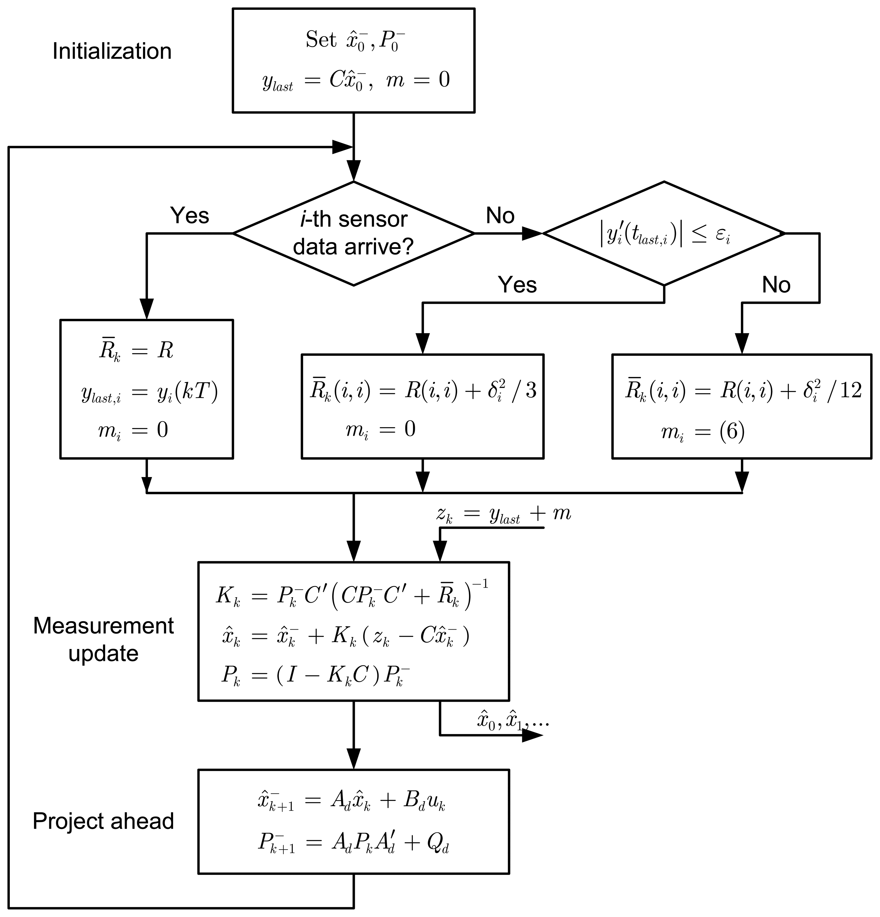
A modified Kalman filter for state estimation at step k, where there is a change in the measurement update part of the discrete Kalman filter algorithm, is given as in the Fig.3 when both (3) and (4) are used in case R ≪ δ². Basic principle of Kalman filters could be found in [10,11]. In Fig.3, we use the discretized plant model is sampled at period T:

$$A_d=e^{AT},B_d=\underset{0}{\overset{T}{\int }}{e}^{Ar}\mathit{\text{Bdr}},$$

Q_d is the process noise covariance of the discretized plant:

$$Q_d=\underset{0}{\overset{T}{\int }}{e}^{Ar}Q{e}^{A^{\prime }r}dr,$$

y_last is the vector of p last received sensor values:

$$y_{\mathit{\text{last}}}={\left[\begin{array}{cccc}{y}_{\mathit{\text{last}},1}& y_{\mathit{\text{last}},2}& \mathrm{\cdots }& y_{\mathit{\text{last}},p}\end{array}\right]}^{\prime },$$

and m is the vector of p men values:

$$m={\left[\begin{array}{cccc}{m}_1& m_2& \mathrm{\cdots }& m_p\end{array}\right]}^{\prime }.$$

In the modified filter above, vector m presents mean value of v_n(t) for all p measurement outputs. In case the filter uses (4) for estimation, m becomes non-zero. In order to satisfy zero mean noise condition, we add m to y_last and consider (y_last+ m) as the measurement values.

The ε_i thresholds determine when the filter uses (4) instead of (3). The smaller ε_i is, the more the filter relies on (4). In practical systems, ε_i thresholds could be determined by monitoring derivative of the sensor output $y_i^{\prime }(t)$.

It is difficult to derive an explicit expression of performance improvement. However, we could say that the error covariance P_k becomes smaller when (4) is used more often. This is because smaller R̅ value in the Kalman filter results in smaller P_k value. We note that (4) is more often used if y(t) is either monotonically increasing or decreasing.

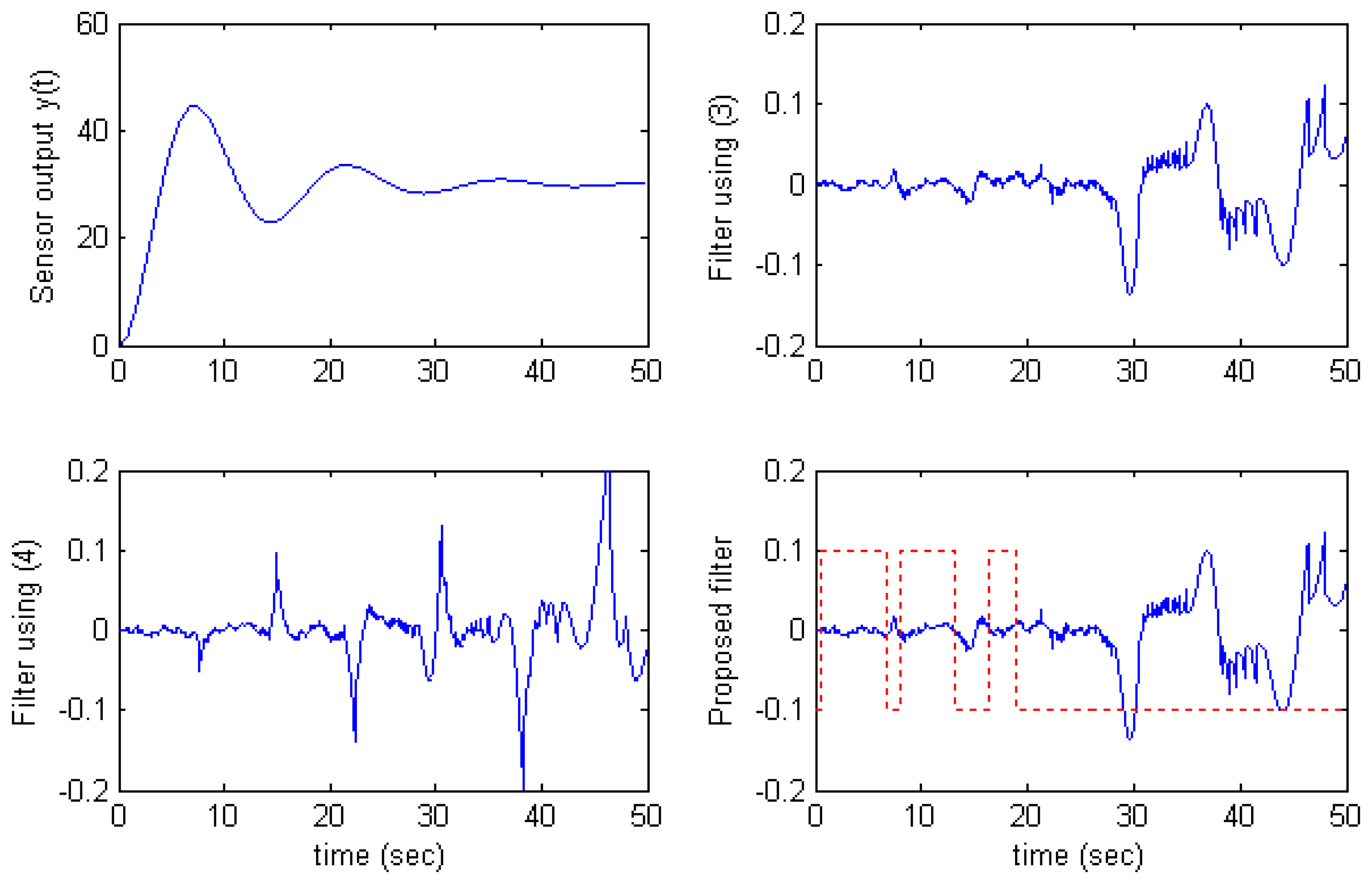
4. Simulation

To verify the proposed filter, we consider an example of the step response of a second-order system where the output is sampled by the SOD method:

$$\begin{array}{l}\dot{x}(t)=\left[\begin{array}{c}0\\ -1/a\end{array}\begin{array}{c}1\\ -b/a\end{array}\right]x(t)+\left[\begin{array}{l}\begin{array}{l}\begin{array}{c}0\\ M/a\end{array}\hfill \end{array}\hfill \end{array}\right]u(t)+w(t)\hfill \\ y(t)=\left[\begin{array}{cc}1& 0\end{array}\right]x(t)+v(t)\hfill \\ Q={10}^{-4},R={10}^{-4},T=10ms\hfill \end{array}$$

The system parameters are given in 3 following cases for performance evaluation:

• M = 30, a =10, b = 10 : overdamped system
• M = 30, a =5, b = 1 : underdamped system
• M = 30, a =5, b = 0 : undamped system

The simulation process is implemented for 50 seconds, and ε = 0.001 for all cases. In each case, we use 3 filters for performance comparison: the filter using (3) only, the filter using (4) only, and the proposed filter. Estimation error is evaluated by the criterion:

$$e={\left(\frac{1}{N}\sum _{k=1}^N{(x_1-{\widehat{x}}_1)}^2\right)}^{1/2}$$

(8)

where x₁ is the reference state, N₌₅₀₀₀.

Estimation errors for different δ values in 3 cases, where the condition R ≪ δ² is satisfied, are given in

Table 1. Estimation error with different δ values in case 1.

	δ = 0.05	δ = 0.1	δ = 0.15	δ = 0.2
n	454	268	185	141
Filter using (3)	2.5643e-004	3.2061e-004	4.6965e-004	5.6528e-004
Filter using (4)	1.9581e-004	2.0124e-004	3.0587e-004	3.5756e-004
Proposed filter	1.9581e-004	2.0123e-004	3.0588e-004	3.5755e-004

n: number of sensor data transmissions

,

Table 2. Estimation error with different δ values in case 2.

	δ = 0.05	δ = 0.01	δ = 0.15	δ = 0.2
n	1168	657	484	370
Filter using (3)	0.9644e-004	2.7051e-004	4.1805e-004	5.5656e-004
Filter using (4)	1.7065e-004	2.9365e-004	4.6972e-004	5.5783e-004
Proposed filter	0.9468e-004	2.6787e-004	4.1551e-004	5.5166e-004

, and

Table 3. Estimation error with different δ values in case 3.

	δ = 0.05	δ = 0.1	δ = 0.15	δ = 0.2
n	4055	3091	1939	1700
Filter using (3)	4.1432e-005	5.1109e-005	4.1805e-005	6.5436e-005
Filter using (4)	4.4961e-005	6.6618e-005	4.6972e-005	8.2118e-005
Proposed filter	3.9019e-005	4.6125e-005	4.1751e-005	6.0537e-005

. We see that estimation performance of the proposed filter is the best and significantly improved in comparison with the filter using (3). For example, in the case of δ = 0.2, estimation error of the proposed filter is reduced 36.75% compared to the filter using (3) in case 1, reduced 0.88% in case 2, and reduced 7.49% in case 3.

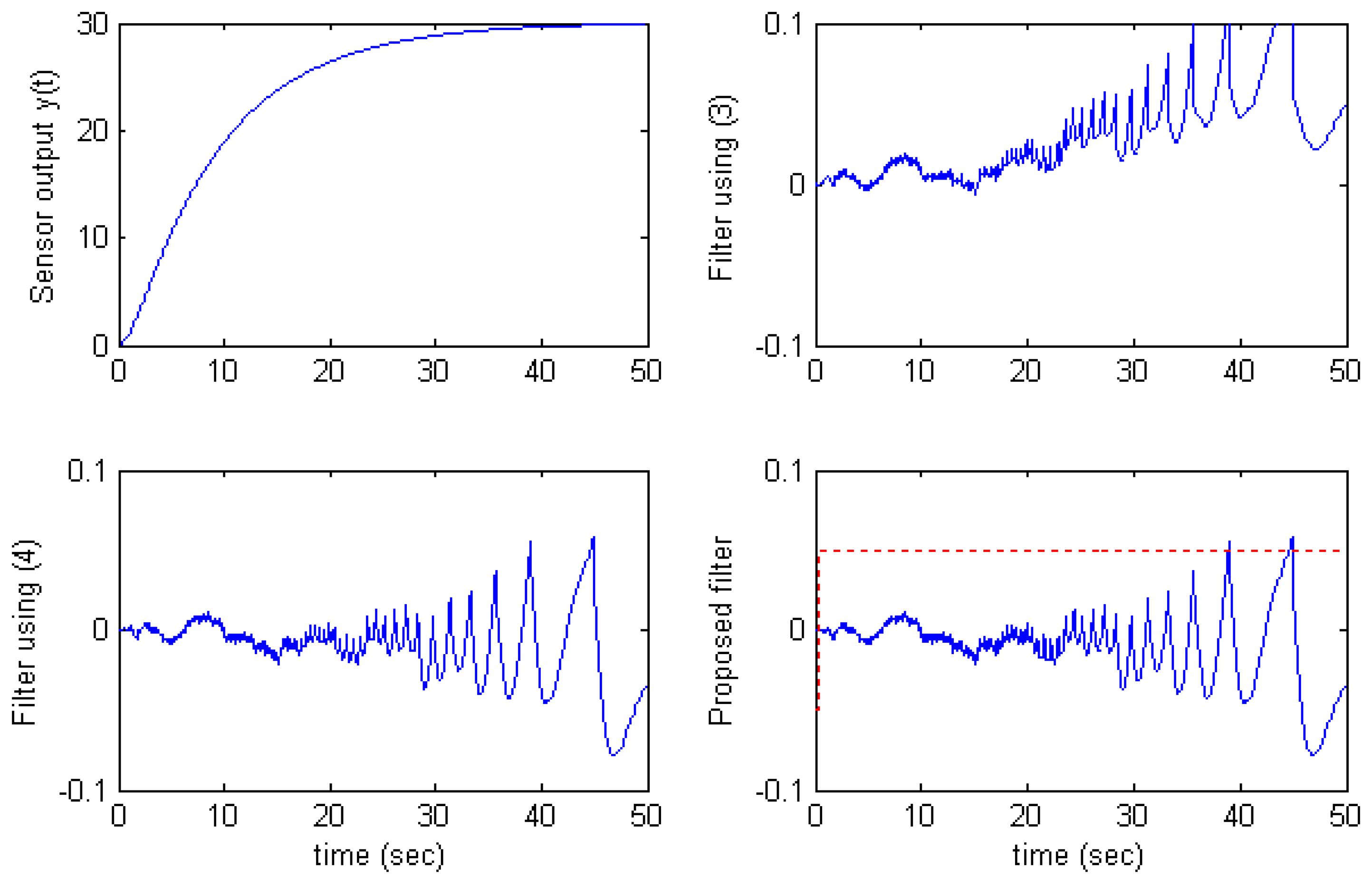
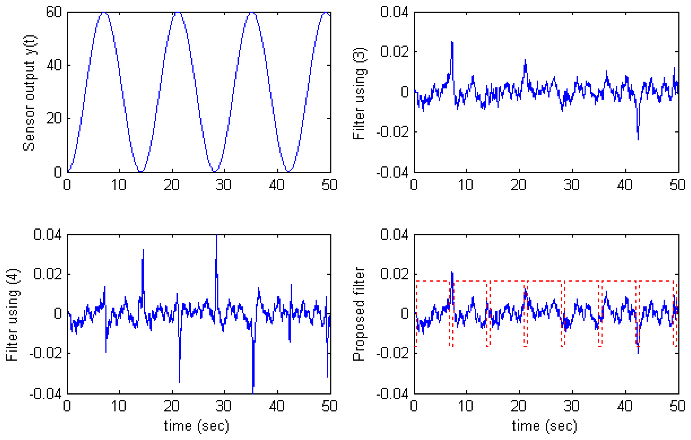
The results also show that the filter using (4) is better than the filter using (3) in case 1, but worse in case 2 and case 3. In theory, the filter using (4) must be always better than the filter using (3). This happens because there exists a delay between the sensor output signal y′(t) and the computed value y′(t_last) in (5). Therefore, if y′(t) changes sign while condition |y(t) − y(t_last)| < δ still holds, the estimator keeps using the old value y′(t_last) whose sign is incorrect compared with y′(t). This makes (6) incorrect, and leads to increase of estimation error. As we see in the Fig.5 and Fig.6, the estimation error of the filter using (4) becomes large at time y′(t) changes the sign.

The proposed filter overcomes this situation by applying the algorithm (7) in which the filter uses (3) at time y′(t) changes sign and uses (4) at other time. The solid line on the proposed filter graphs in Fig.4, Fig.5, and Fig.6 presents the sign of Selector (7). That is, Selector > 0 denotes that the filter uses (4) and Selector < 0 denotes that the filter uses (3).

5. Conclusion

In this paper, the state estimation problem with SOD transmission method over the network has been considered. The main objective of this paper is how to reduce the estimation performance degradation when the SOD transmission method is used. With given δ value and measurement noise, R a suitable new noise is computed and compensated to the estimator so that estimation error is as small as possible. Accordingly, not only sensor data transmission rate can be significantly reduced, but also estimation performance degradation is relatively small. Through the simulations, it is shown that estimation performance of the proposed method is better than that of [5], where the total number of sensor data transmissions is identical.