Article

Send-On-Delta Concept: An Event-Based Data Reporting Strategy

AGH University of Science and Technology, Department of Electronics, al. Mickiewicza 30, 30-059 Krakow, Poland
Sensors 2006, 6(1), 49-63; https://doi.org/10.3390/s6010049
Submission received: 7 December 2005 / Accepted: 18 January 2006 / Published: 20 January 2006
(This article belongs to the Special Issue Wireless Sensor Networks and Platforms)

Abstract

:
The paper addresses the issue of the send-on-delta data collecting strategy to capture information from the environment. Send-on-delta concept is the signal-dependent temporal sampling scheme, where the sampling is triggered if the signal deviates by delta defined as the significant change of its value. It is an attractive scheme for wireless sensor networking due to effective energy consumption. The quantitative evaluations of send-on-delta scheme for a general type continuous-time bandlimited signal are presented in the paper. The bounds on the mean traffic of reports for a given signal, and assumed sampling resolution, are evaluated. Furthermore, the send-on-delta effectiveness, defined as the reduction of the mean rate of reports in comparison to the periodic sampling for a given resolution, is derived. It is shown that the lower bound of the send-on-delta effectiveness (i.e. the guaranteed reduction) is independent of the sampling resolution, and constitutes the built-in feature of the input signal. The calculation of the effectiveness for standard signals, that model the state evolution of dynamic environment in time, is exemplified. Finally, the example of send-on-delta programming is shown.

1. Introduction

The primary objective of sensor networks is to sample the residing environment and send updates with the most recent information to data collecting center(s) for further processing. As is well-known, a main constraint of wireless sensor devices is limited battery life. Usually it is either impossible or impractical to replace batteries so the operational lifetime of the sensor device is equal to its battery life. The only option to lengthen the sensor lifetime is to reduce the waste of energy in device operation.
Wireless communication is a major source of energy consumption. Since every message uses up the low device energy resources, the number of messages sent through the sensor network should be as low as possible. It is worth being aware that every bit transmitted can reduce the lifetime of the wireless sensor network [12]. Wireless communication consumes more energy than information processing. In a typical scenario, a sensor node can execute 3000 instructions for the same energy cost of sending a single bit at the distance of 100 meters by radio [15]. Therefore, in order to maximize the lifetime of the sensor devices, it is critical to maximize the usefulness of every bit transmitted or received [12].
The effective way to decrease energy consumption is the reduction of the network traffic originated out of a sensor node without degrading the resolution of observations reported from the environment. It is possible by a use of signal-dependent sampling schemes, where sampling occurs “when it is required” rather than in equidistant time intervals.
Basing on both data collection paradigms, a classification of sensor networks into proactive and reactive ones has been proposed [16]. Proactive networks continuously monitor the environment and thus have data to be sent at a constant rate. In the reactive network, nodes send new reports only when the variable being monitored increases or decreases beyond a threshold. The latter is sometimes called the send-on-delta scheme.
The paper addresses the issue of send-on-delta data collecting strategy to capture information from the environment. Send-on-delta concept is the most natural signal-dependent temporal sampling scheme. According to this scheme the sampling is triggered if the signal deviates by delta, defined as a significant change of its value (e.g. 1°C) in relation to the most recent sample. Thus, the sensor node does not broadcast a new message until the input signal remains within a certain interval of confidence.
The level-crossing sampling is not new and has been known at least since the late 1950s, when Ellis noticed, that “the most suitable sampling is by transmission of only significant data, as the new value obtained when the signal is changed by a given increment” [20]. Consequently, “it is not necessary to sample periodically, but only when quantized data change from one possible value to the next” [20]. Various terms are used to express such a sampling strategy: the event-based sampling [1,2,3,17], the level-crossing sampling [5,18,24], the magnitude-driven sampling [3], and sometimes, the sampling in the amplitude domain. Recently, Aström and Bernhardsson suggest a term Lebesgue sampling, since the discrete representation of a continuous-time signal by levels equally distributed in the amplitude domain resembles the Lebesgue method of integration in mathematics [22]. Using the same convention of terminology the periodic scheme is called Riemann sampling [22]. The variety of existing terminology shows that it is really a generic concept adapted to a broad spectrum of technology and applications. In the sensor/control networking community the magnitude-driven/level-crossing sampling is known as the send-on-delta [6,7,13] or deadbands [11].
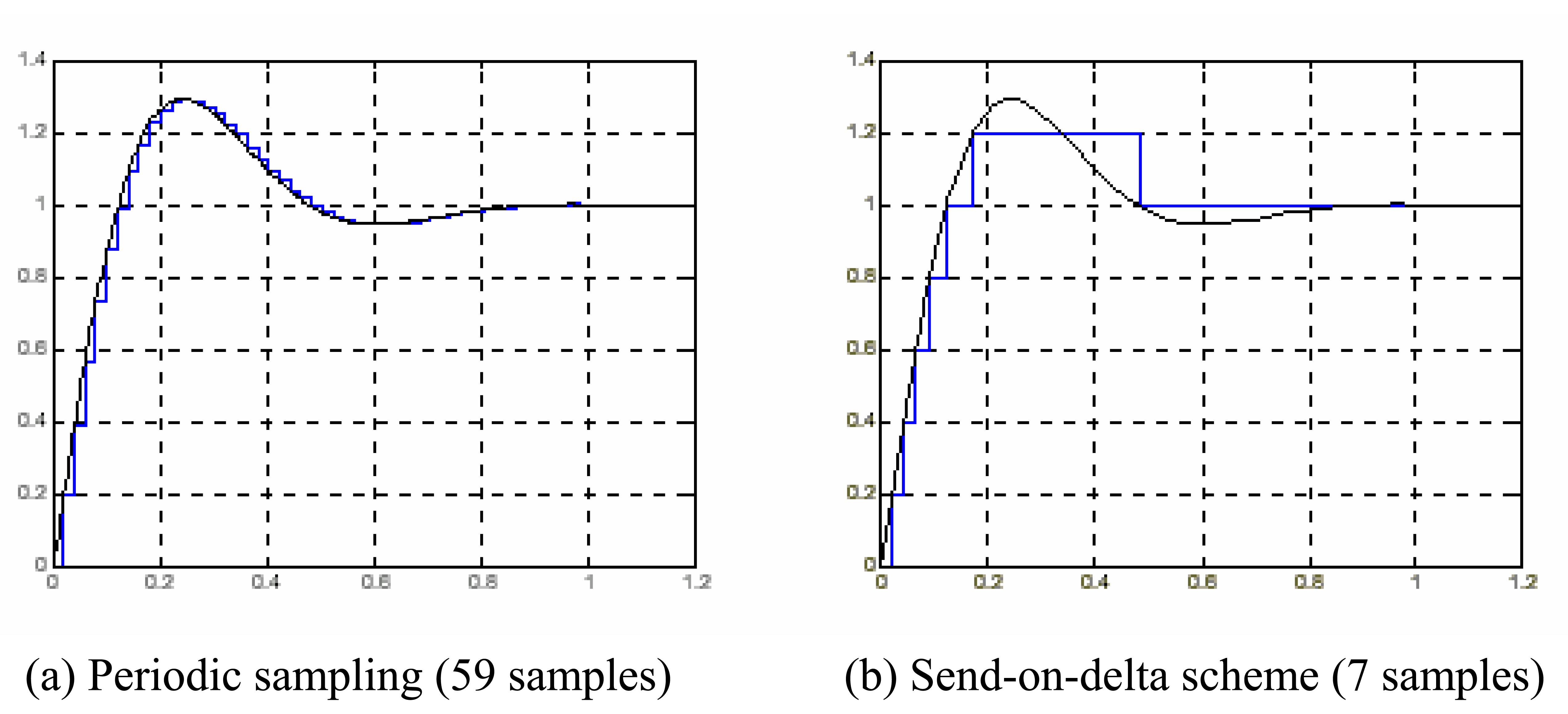
The send-on-delta scheme is used in many wireless sensor network applications. It is intuitively comprehensible that a use of the send-on-delta concept instead of traditional periodic updates reduces the mean rate of messages generated by a sensor node [3]. The reduction is significant for burst signals, defined as a type of signals that do not change, much or at all, for most of the time. Hence, the send-on-delta data collection is less demanding in terms of wireless communication since only significant changes of the input signal are propagated to a higher processing infrastructure.
The problem of waste of energy due to the transmission of redundant data is characterized in [6] as overtransmitting. This term has been developed following the convention of terminology used in the sensor network protocols, where overhearing describes the effect of packets reception by nodes that are not their intended recipients.
The send-on-delta-based data acquisition might be used together with switching the sensor node to low-power state and the event-driven wake up to reduce waste of energy when the input signal is lazy. The analysis of energy savings and possible sensor lifetime increase in send-on-delta-based reporting is presented in [6].
The send-on-delta strategy of the environmental monitoring is often a built-in feature of smart sensor devices. Some sensor/control networking technologies with the event-triggered architecture is equipped with the magnitude-driven input perception. A typical example is LonWorks/EIA-709 technology supporting programming resources for event detection and processing [8,13,14].
LonWorks technology allows a node to go to sleep and to wake up if specified events occur. Each node sleeps autonomously calling sleep() function [8]. The node can wake up when some activity in local environment (on I/O port), or in the communication channel is detected. However, the node can be configured to ignore incoming messages, e.g. when a sensor node is programmed as a source of messages only, and is not interested in message receiving.
The research area related to the send-on-delta sampling scheme is the level-crossing problem, i.e. the evaluation of statistical temporal properties of crossings of a certain level by random signals [23]. However, the results derived for the level-crossing problem cannot be applied directly to the send-on-delta scheme since the former deals with the issue of the single level crossings, and the latter concerns the crossings of multiple levels distributed in the amplitude domain.
Recently, the new research areas related to the level-crossing sampling have been initiated. A new type of signal processing problem related to the send-on-delta/event-based sampling is studied in [17], where the purpose of spectral analysis in the signal amplitude domain is introduced and exemplified. Finally, a new promising application of the level-crossing sampling is the asynchronous analog-to-digital conversion [18,21], where the intersampling intervals instead of the signal amplitude are quantized according to the resolution of a timer, the purpose of which is only to date the samples. It announces a drastic change in the standard signal and data processing and the development of a new research area – asynchronous signal processing [21].
In this paper, the quantitative evaluations of the send-on-delta scheme for a general type continuous-time bandlimited signal are presented. First, Section 2 highlights the motivation of using the send-on-delta paradigm. In Section 3, the lower and the upper bounds on the mean traffic of messages for a given signal, and assumed sampling resolution, are evaluated. The analytic expressions estimate a balance between the traffic rate and the send-on-delta sampling resolution. Furthermore, in Section 4, the send-on-delta effectiveness, defined as the reduction of the mean rate of messages in comparison to the periodic sampling for a given resolution, is derived. In particular, it is shown that the lower bound of the send-on-delta effectiveness (i.e. the guaranteed reduction) is independent of the sampling resolution, and constitutes the built-in feature of the input signal. The calculation of the effectiveness for standard signals, that model the state evolution of dynamic environment in time, is exemplified. Finally, the example of send-on-delta programming is shown.

2. Motivation of use of the periodic sampling and the send-on-delta concept

One of the most prominent and comprehensive ways of data collection in sensor networks is to extract raw sensor readings periodically. The uniform time-triggered data collection is assumed by most current protocols for wireless sensor networks. The sampling period depends mainly on how fast process can vary and what characteristics need to be captured. The selection of sampling period bases on the worst-case approach, and is adjusted to the fastest possible signal change.

2.1. Typical applications of the periodic data collection

Since the concepts of time and speed play a major role in the process control area, the synchronous sampling is natural in real-time control applications, where the system interacts in a feedback with the controlled object within imposed time constraints. The important reason is the existence of a well-established and mature system theory for periodic sampled control systems. The analysis and design of such sampled systems are relatively simple because the closed-loop system becomes linear and periodic for linear time-invariant processes [19]. Reservation protocols are natural for message transport in the sensor network with equidistant sampling data collection.
From the point of view of real-time software, the periodic sampling supports the time-triggered architecture (TTA). Time is indeed a critical issue for real-time applications so the explicit management of time at the basic level supports the evaluation of the temporal properties of real-time software [9]. Thus, recommendations for software architecture harmonize with control theory issues.
Although periodic sampling is a crucial approach in most sensor/control and signal processing applications, the implicit idea of its use relying on the assumption about regularity of environment evolution in the time, is usually invalid. Sensor networks have to deal with high system dynamics. The environment being sensed is bursty by nature so sending data periodically when nothing significant has happened in the process seems to be an evident waste of communication, processing and energy resources. Significant oversampling occurs, for example, when the controlled object is in the equilibrium and state variables do not change considerably.
The other problem associated with synchronous sampling applications is the phase relation of sampling instants among multiple sensor nodes. A random access sensor network is prone to repeated collisions if more than one node operates with the same or similar sampling frequencies. Thus, the instants when data reports are triggered in several nodes, should be distributed in the time in order to desynchronize the traffic.
Finally, it is no point to sample environment in the strict uniform time-triggered regime if the jitter of transmission delay is greater than the sampling period since temporal order of observations can be disturbed. Delay jitter is significant in random access networks with the backoff-based collision avoidance, or when messages are transmitted across field buses, computer networks, or even the Internet.

2.3. Problems of send-on-delta-based acquisition

A sensor network is essentially an event-based system. Events of interest occur in a sensor field asynchronously with regard to a priori selected sampling points. Therefore, the signal-dependent schemes, where the sampling instants are correlated with the stimuli coming from the environment, are more natural than the time-triggered ones, which periodic sampling exemplifies. In the signal-dependent sampling, the system input is fed by signal amplitude variations so the temporal density of sampling operations varies in the time, and is determined by input signal changes.
The send-on-delta concept might be used with several network protocols. For example, in LonWorks systems, the send-on-delta-based reports are transmitted over the CSMA-based channel [5]. On the other hand, the FDMA scheme is proposed for a protocol presented in [6]. In general, the send-on-delta concept corresponds well to the event-based nature of random access protocols, where every node decides to transmit autonomously “when it is required”.
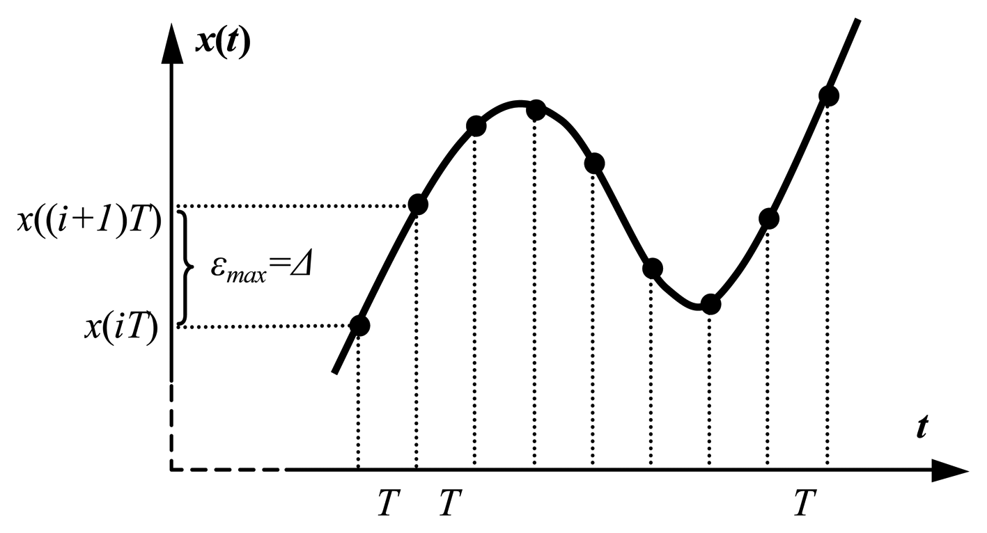
Send-on-delta strategy is sometimes implemented in sensor devices using the compound architecture for data acquisition. First, the continuous-time signal is sampled using the periodic scheme. On the top of it, the event-triggered communication and processing activities are implemented, that is, a detection of a significant change in a set of samples is performed. The compound approach, where the asynchronous events are presynchronized by background periodic sampling, is called the “upwardevent-driven architecture [9]. Such a compound architecture of send-on-delta implementation is used in many sensor networking applications, e.g. in LonWorks technology.

3. Send-on-delta principle
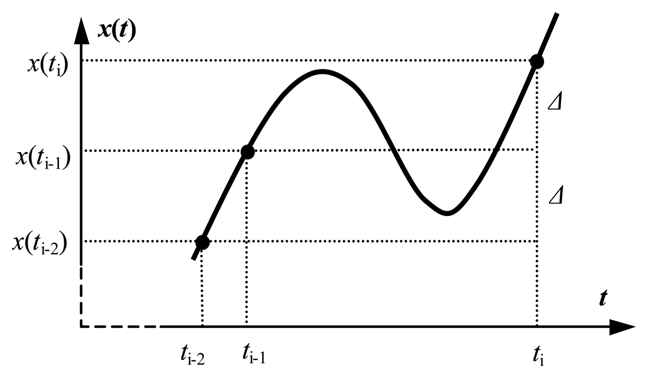
Using the send-on-delta concept, a continuous-time bandlimited signal x(t) is sampled and a new report is sent, when the value of the physical variable being sensed deviates from the value included in the most recent report by an interval of confidence ± Δ, called the threshold, or delta, where Δ > 0 (Fig. 1).
Thus, there is a constant difference equal to Δ between signal values included in consecutive updates:
| x ( t i ) x ( t i 1 ) | = Δ
where x(ti) is the ith signal sample; i = 1,2,…,n.
The threshold Δ is a design parameter that determines the resolution of signal observations. The smaller threshold Δ, the higher resolution of input signal tracking. The digitized samples including the current signal value x(ti) and the protocol overhead are sent in messages through the sensor network.
Since by definition, the send-on-delta sampling is triggered by asynchronous events (crossings of the sampling levels), the time is the dependent variable in system modelling. Meanwhile, the communication requirements relate to temporal properties, e.g. measures that evaluate demands for the required network communication bandwidth.

3.2. Communication Bandwidth Requirements

One of the main parameters describing the send-on-delta concept is the mean rate of messages, λ, originated out of a node sensing a particular continuous-time physical variable with the resolution in the value domain equal to Δ. The mean rate of messages is simply defined as the mean number of samples per a unit of time calculated for a certain time interval (t0,tn).
The mean rate of messages λ cannot be estimated analytically for a general type signal. However, either the upper bound λmax, or the lower bound λmin of λ might be evaluated according to the following expression [4]:
λ min = λ ' 2 ν < λ λ ' = λ max
where v,vR is the local extrema density, i.e. the average number of signal peaks (maxima and minima) in a time unit.

3.2.1. Upper bound on the mean rate of messages

The upper bound λmax equals λ ′, which is defined as follows [3]:
λ ' = | x ' ( t ) | ¯ Δ ,
where | x ( t ) ¯ | is the average slope of the signal, that is, the mean of the absolute value of the first time-derivative of the signal x(t) in a time interval (t0,tn):
| x ' ( t ) | ¯ = 1 t n t 0 t 0 t n | x ' ( t ) | d t
By the definition (see (3)), the measure λ′ is expressed by two factors:
-
the mean of the absolute value of the first signal time-derivative during a time interval (t0,tn):
| x ' ( t ) | ¯ = 1 t n t 0 t 0 t n | x ' ( t ) | d t
-
the resolution Δ of the sampling in the value domain, or the threshold, which is a difference between the consecutive sampling levels, see (1).
As expected, the larger threshold Δ, the lower sensing resolution, and the lower mean rate of messages λ. The measure λ′ has highly intuitive interpretation. Namely, it is the average slope of the sampled signal x(t) normalized to the threshold Δ. Since λ′ overestimates λ, it represents the worst-case mean rate of messages for a certain threshold Δ. Next, as follows from the formula (2) and (3), λ approaches λ′, if the threshold Δ is small, because:
1 Δ | x ' ( t ) | ¯ 2 ν .
Finally, if Δ→ 0, then λλ′, because:
lim Δ 0 ( λ ' λ ) = inf Δ 0 ( λ ' λ ) = 0 .
Thus, if the threshold Δ approaches zero, then the mean observation rate λ converges to its upper bound λ′.

3.2.2. Lower bound on the mean rate of messages

The lower bound λmin on mean rate of messages equals to (λ′ − 2v) and depends on the density of peaks in the signal being sensed by the sensor node. To be precise, the lower bound λmin is defined for such a threshold Δ that:
Δ < | x ' ( t ) | ¯ 2 ν
If this inequality is violated, the level-crossing sampling might not be triggered since the signal value can vary within a region between two consecutive sampling levels.
The uncertainty (λmaxλmin) of the analytic evaluation of the mean rate of messages λ in send-on-delta data collecting strategy in the presented approach defined as:
λ max λ min = 2 ν ,
is a function of the mean density of peaks in the signal.
In particular, if v = 0 (i.e. the signal x(t) is a monotone increasing of decreasing function of the time), the mean rate of messages λ is perfectly evaluated (λmax =λ = λmin) and equal to λ′. Some signals in dynamic systems meet this assumption, e.g. the first-order or higher order over-damped or critically damped step-responses.
Note that in order to estimate all the parameters λ, λmin, λmax, only the average slope of the signal | x ( t ) | ¯, and the mean peak density v have to be calculated since the threshold is a design parameter. Both parameters, | x ( t ) | ¯ and v, can be found analytically for many common signals, either deterministic, or random ones.
Summing up, the mean rate of messages λ in send-on-delta concept, cannot be estimated perfectly using the analytic approach for a general type signal. However, the upper bound, and the lower bound on λ can be found basing on signal parameters. Moreover, if the sampling resolution is high (i.e. the threshold Δ is small), the mean sampling rate λ approaches asymptotically λ′. On the other hand, if the signal x(t) is a monotone increasing of decreasing function of the time, the mean rate of messages λ is perfectly evaluated and equal to λ′.

4. Send-on-delta effectiveness against periodic data collection

As it was emphasized in the introduction, a better utilization of system resources is one of the most important benefits of send-on-delta data collecting strategy. Thus, a natural question arises, how much effective is the send-on-delta scheme in relation to the periodic one? The answer to this question determines how much communication bandwidth and energy can be saved, if the periodic reporting is replaced with the send-on-delta observations. We present below the comparison of both sampling patterns for the same signal tracking resolution.

4.1. Selection of sampling period in periodic sampling

In the periodic sampling, the resolution of the sensed signal in the value domain is defined by the maximum difference between values included in the consecutive reports, and is controlled by the sampling period. The sampling period T is adjusted to the fastest change of a signal during a time interval (t0,tn) so the following relationship is valid (Fig. 2):
| x ( t ) | max T = ε max ,
where |x′(t)|max is the maximum slope of the sampled signal, i.e. the maximum of the absolute value of the first signal derivative in relation to the time during an interval (t0,tn), εmax is the maximum difference between values included in the consecutive reports, i.e. resolution of signal measurements.
Thus, using the periodic scheme, the sampling frequency, i.e. the number of samples in a time unit, amounts to:
λ T = 1 T = | x ( t ) | max ε max .

4.2. Send-on-delta scheme effectiveness

We define intuitively the effectiveness p of send-on-delta scheme as the ratio of the sampling frequency in the periodic scheme λT and the mean rate of messages λ in send-on-delta scheme [3]:
p = λ T λ
The sampling effectiveness (i.e. the reduction of the mean rate of messages if the periodic reporting is replaced with the send-on-delta observations) for the same resolution of environment observation εmax = Δ in both sampling schemes is found after setting (2) and (11) to (12). Thus, the lower and upper constraints for the sampling rate reduction are as follows:
p min = | x ( t ) | max | x ( t ) | < p | x ( t ) | max | x ( t ) | 2 v E = p max ,
To be precise, the right inequality (the expression evaluating pmax) is valid if the condition (8) is met. In particular, if v = 0 (i.e., the signal x(t) is a monotone increasing of decreasing function of the time), then pmin = pmax = p, and the sampling effectiveness is independent of the threshold Δ.
Since all the parameters required for effectiveness estimation (i.e. either the average or the maximum slope of the sensed signal, and the mean peaks density) are defined also for random processes, all the evaluations (i.e. formulas (2), (11), (13)) are valid either for deterministic, or stochastic signals.

4.3. Examples of sampling effectiveness calculation

Fig. 3 shows simulative comparison of the number of samples taken in a periodic sampling (a), and send-on-delta scheme (b), for the same continuous-time test signal. The resolution is the same in both cases (εmax = Δ = 0.2). Whereas using the periodic sampling pattern 59 samples has to be taken, in send-on-delta scheme only 7 sampling operations are triggered.
The test signal is the step-response of the second-order underdamped closed-loop system, given by the open-loop transfer function F(s) = (10s + 100)/s2. The signal x(t) has the following form in the time domain:
x ( t ) = 1 + 3 3 e 5 t sin 5 3 t e 5 t cos 5 3 t
and is presented on the Fig. 3 (a,b).
The send-on-delta effectiveness calculated on a basis of simulation results shown on Fig. 3 equals:
p ( Δ = 0.2 ) = 59 / 7 8.4
The simulation has been run for the time interval (0;1.2[sec]), when the transient component of the test signal dies out and the signal becomes nearly constant at the end of the selected time interval.
For a comparison, the minimum send-on-delta effectiveness for this particular test signal and the same time interval (0;1.2[sec]) might be predicted basing on the analytical formula (13):
p min = | x ( t ) | max | x ( t ) | = 12 0 1.2 | 10 3 e 5 t ( 3 cos [ 5 3 t ] + 3 sin [ 5 3 t ] ) | 3 d t 7.02
Both results are consistent. Note that the analytic formula estimates the minimum, or guaranteed effectiveness (i.e. effectiveness for the infinite small threshold), whereas the simulation has been run for the finite threshold εmax = Δ = 0.2, therefore p(Δ = 0.2)> pmin(Δ → 0).

4.4. Derivation of effectiveness for standard signals modeling the dynamic environment

On a basis of the formula (13) we found the analytic solutions of the guaranteed send-on-delta effectiveness for particular time responses of the first and the second-order dynamic systems, which are models of environment temporal evolution in many sensor networking applications. The results are shown in Table 1.
The send-on-delta effectiveness for step-responses of the following systems are calculated:
-
the first-order system,
-
the second-order underdamped system (0 < ξ < 1, where ξ is a damping factor) with the same time constants,
-
the second-order underdamped system with different time constants,
-
the second-order undamped system (ξ = 0).
The send-on-delta effectiveness calculated for the time interval (0,tn) is a function of η (or η1 and η2 for a system with different time constants), which is the length of the considered time interval tn normalized to the time constants (η = tn/T, η1 = tn/T1, η2 = tn/T2). Except the step-response of the second-order undamped system (ξ = 0), which is the harmonic signal, all the signals presented in Table 1 are monotonic in the time (v = 0). Thus, the effectiveness Pmin = Pmax = p is independent of the sampling resolution. Note that the guaranteed effectiveness for the pure harmonic signal, amounts to π/2=1.57.
Table 2 shows the send-on-delta effectiveness calculated for selected time intervals (0,tn). The time interval selection (except the undamped system) is based on the assumption that tn represents the settling time of a system, i.e. the time required for the step response to stay within a specified percentage of its final value. The percentage is shown in the first column, e.g. for the second-order underdamped system with the same time constants tn = 5T is set, because x(5T) = 0.959x0. For the second-order underdamped system with different time constants T1/T2 = 7/5 is assumed, since x(5T1 = 7T2) = 0.97x0.
The presented results show that the reduction of the traffic in the sensor network, where the send-on-delta sampling is used, ranges between 1.57 and 5.85 for signals selected in Table 2.
As follows from the send-on-delta scheme, the time intervals between consecutive messages are not equally spaced in the time domain, but they depend on the current signal dynamics. In closed-loop control systems a controlled variable changes significantly especially when a new reference value is set. Then a burst of event-based observations starts, because the system drives the controlled object to the new equilibrium state. If the controlled variable reaches its new steady-state value, the burst of observations finishes. During the equilibrium state, if the disturbance is small, and the controlled variable is kept at nearly constant level, only rare hearbeat sampling occur to indicate that the sensor node is still healthy e.g. see recommendations for LonWorks technology in [13].

5. The example of send-on-delta programming

The send-on-delta monitoring is a built-in feature of many intelligent sensor devices. As it was mentioned, some sensor/control networking technologies with event-driven architecture are equipped with possibility of the event-based input perception. A typical example is LonWork/EIA-709 technology supporting programming resources for event detection and processing [5,13].
The Local Operating Networks (LonWorks) application programming language (Neuron C) offers the special predefined event io_changes dedicated to the monitoring of I/O objects [8]. The io_changes event is a programming event detector. It evaluates to the positive logical level when the value read from the specified I/O object changes its state.
The io_changes event with to modifier supports the event-driven input monitoring when the I/O object deviates from the reference value by a relative value. The threshold can be specified by shift-expr, which is a Neuron C expression. The shift-expr might be constant but may also vary in consecutive comparisons. Thus, either static or dynamic send-on-delta monitoring is possible to implement.
When the io_changes event is evaluated, an input value for the I/O object can be accessed using the built-in variable input_value and can be broadcasted using the network variables to application programs resided in remote nodes. The heartbeat update might be supported using propagate() built-in function.

Conclusion

The paper summarizes the quantitative evaluations of the send-on-delta sampling rate and its superiority against periodic data collection in terms of the number of samples per time unit. It was displayed that the guaranteed reduction of reports is a built-in feature of the process being sensed. The knowledge about the expected bandwidth demands and the possible savings allows to predict a priori its potential usefulness for a particular application scenario. Since “every bit transmitted reduces the lifetime of the wireless sensor device”, send-on-delta concept becomes an attractive sampling scheme for today's wireless sensor networking applications.

References and Notes

  1. Arzén, K.E. A simple event-based PID controller. Proceedings of IFAC World Congress 1999, 18, 423–428. [Google Scholar]
  2. Bernhardsson, B. Event triggered sampling. Research problem formulations in the DICOSMOS project; Törngren, M., Sanfridson, M., Eds.; Lund Institute of Technology, 1998. http://www.md.kth.se/∼mis/dicosmos/publications/ET-sampling.pdf.
  3. Miskowicz, M. Analytical approximation of the uniform magnitude-driven sampling effectiveness. In Proceedings of IEEE International Symposium on Industrial Electronics ISIE'2004; Ajaccio, France, 2004; pp. 407–10. [Google Scholar]
  4. Miskowicz, M. Bandwidth requirements for event-driven observations of continuous-time variable. In Proceedings of IFAC Workshop on Discrete-Event Systems; Reims, France, 2004; pp. 475–480. [Google Scholar]
  5. Miskowicz, M.; Golanski, R. LON Technology in Wireless Sensor Networking Applications. Sensors 2006, 6, 30–48. [Google Scholar]
  6. Neugebauer, M.; Kabitzsch, K. A new protocol for a low power sensor network. Proceedings of IEEE International Performance, Computing and Communications Conference IPCCC'2004; Phoenix, Arizona, 2004; pp. 393–399. http://web.inf.tu-dresden.de/∼mn7/publications/neugebauer04protocolLowPower.pdf.
  7. Plönnigs, J.; Neugebauer, M.; Kabitzsch, K. A traffic model for networked devices in the building automation. Proceedings of IEEE International Workshop on Factory Communication Systems WFCS'2004; Vienna, Austria, 2004; pp. 137–145. http://web.inf.tu-dresden.de/∼mn7/publications/ploeNeuKab04WFCSArrivalRates.pdf.
  8. Neuron C Reference Guide; Echelon Corporation, 1995. http://www.echelon.com/support/documentation/manuals/devtools/078-0140-02E.pdf.
  9. De Paoli, F.; Tisato, F. On the complementary nature of event-driven and time-driven models. Control Engineering Practice 1996, 4, 847–854. [Google Scholar]
  10. Kopetz, H. Real-time systems. Design principles for distributed embedded applications.; Kluwer Academic Publishers: Boston, 1997. [Google Scholar]
  11. Otanez, P.; Moyne, J.; Tilbury, D. Using deadbands to reduce communication in networked control systems. Proceedings of American Control Conference ACC'2002; Anchorage, USA, 2002; 4, pp. 3015–3020. http://www.mae.cornell.edu/SEC/Otanez/Publications/otanez_using_2002.pdf.
  12. Elson, J.; Estrin, D. An address-free architecture for dynamic sensor networks. Technical Report 00-724. University of Southern California: Computer Science Department, 2000. http://citeseer.ist.psu.edu/cache/papers/cs/14766/http:zSzzSzwww.circlemud.orgzSz∼jelsonzSzwritingszSzafa-tr.pdf/elson00addressfree.pdf.
  13. Layer 7 LonMark Interoperability Guidelines; Ver. 3.2. LonMark Interoperability Association, 2002. http://www.lonmark.com/press/download/LYR732.pdf.
  14. LonWorks Technology Device Data; Rev. 4; Motorola, 1997.
  15. Zheng, R.; Hou, J.; Li, N. Power management and power control in wireless networks. Ad Hoc and Sensor Networks. Pan, Y., Xiao, Y., Eds.; Nova Science Publishers, 2004. http://coco.cs.uh.edu/publications/files/power_management-chapter.pdf.
  16. Manjeshwar, A.; Agrawal, D. P. TEEN: a routing protocol for enhanced efficiency in wireless sensor networks. Proceedings of International Parallel Distributed Processing Symposium IPDPS'2001; San Francisco, USA, 2001; pp. 189–199. http://network.chonnam.ac.kr/seminar/Lab_Seminar/Data/00925197.pdf.
  17. Persson, N.; Gustafsson, F. Event-based sampling with application to monitoring pressure in pneumatic tires. In Proceedings of IEEE International Conference on Acoustics, Speech, and Signal Processing ICASSP'2001; Salt Lake City, USA, 2001; pp. 3885–3888. [Google Scholar]
  18. Sayiner, N.; Sorensen, H.V.; Viswanathan, T.R. A level-crossing sampling scheme for A/D conversion. IEEE Transactions on Circuits & Systems II-Analog & Digital Signal Processing 1996, 43, 335–9. [Google Scholar]
  19. Aström, K.J.; Wittenmark, B. Computer-Controlled Systems: Theory and Design., 3rd edition; Printice Hall: New Jersey, 1997. [Google Scholar]
  20. Ellis, P.H. Extension of phase plane analysis to quantized systems. IRE Transactions on Automatic Control 1959, 4, 43–59. [Google Scholar]
  21. Allier, E.; Sicard, G.; Fesquet, L.; Renaudin, M. A new class of asynchronous a/d converters based on time quantization. In Proceedings of International Symposium on Asynchronous Circuits and Systems ASYNC'03; Vancouver, Canada, 2003; pp. 196–205. [Google Scholar]
  22. Aström, K.J.; Bernhardsson, B. Systems with Lebesgue sampling. In Directions in mathematical systems theory and optimization; Rantzer, A., Byrnes, C.I., Eds.; Springer: Berlin, 2003; Chapter 1; pp. 1–13. [Google Scholar]
  23. Blake, I.F.; Lindsey, W.C. Level-crossing problems for random processes. IEEE Transactions on Information Theory 1973, 3, 295–315. [Google Scholar]
  24. Mark, J.; Todd, T. A Nonuniform Sampling Approach to Data Compression. IEEE Transactions on Communications 1981, 29, 24–32. [Google Scholar]
Figure 1. The principle of the send-on-delta sensor reporting scheme.
Sensors 06 00049f1
Figure 2. The selection of a sampling period in the periodic scheme. The sampling period T is defined by the fastest change of the signal. εmax is assumed to be equal to Δ (see Fig. 1).
Sensors 06 00049f2
Figure 3. Comparison of the number of samples in a periodic (a), and send-on-delta scheme (b), for the same continuous-time test signal. The resolution of signal tracking in both scheme is the same and equals to 0.2.
Sensors 06 00049f3
Table 1. The send-on-delta effectiveness for some time responses of the first and the second-order dynamic systems calculated for the time interval (0,tn), where η = tn/T, η1 = tn/T1, η2 = tn/T2.
Type of signalSignalSend-on-delta effectiveness
Step-response of the first-order system x ( t ) = x 0 ( 1 e t T ) p = η 1 e η
Step-response of the second-order underdamped system (the same time constants) x ( t ) = x 0 [ 1 ( 1 + t T ) e t T ] p = η e e 1 η ( 1 + η )
Step-response of the second-order underdamped system (different time constants) x ( t ) = x 0 ( 1 + T 1 T 2 T 1 e t T 1 + T 2 T 2 T 1 e t T 2 ) p = 2 1 η 1 ( 1 e η 1 ) + 1 η 2 ( 1 e η 2 )
Step-response of the second-order undamped systemx(t) = x0(1−cos ωnt)Pmin = π/2 = 1.57
tn = m π/2ωn; mN
Table 2. The send-on-delta effectiveness for selected time intervals (0,tn).
SignalSend-on-delta effectiveness for selected time intervals
x ( t ) = x 0 ( 1 e t T ) x ( 3 T ) = 0.95 x 0P(η = 3) = 3.16
where: η = tn/T
x ( t ) = x 0 [ 1 ( 1 + t T ) e t T ] x ( 5 T ) = 0.959 x 0p(λ = 5) = 1.92
where: η1 = tn/T1
x ( t ) = x 0 ( 1 + T 1 T 2 T 1 e t T 1 + T 2 T 2 T 1 e t T 2 ) for T 1 / T 2 = 7 / 5 ; x ( 5 T 1 = 7 T 2 ) = 0.97 x 0p(λ1 = 5, λ2 = 7) = 5.85
where:
η1 = tn/T1, η2 = tn/T2
x(t) = x0(1−cosωnt)pmin = π/2 = 1.57

