Overview of Sensors and Needs for Environmental Monitoring

Abstract
:Introduction
Market survey
Regulatory requirements, standards and policies
Drinking water
Storm water monitoring
National pretreatment program monitoring
Ambient air qality
Sensor technologies for environmental monitoring
Trace metal sensors
-Nanoelectrode array
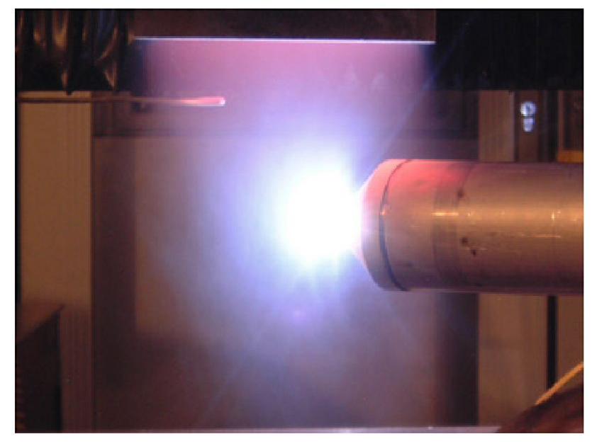
-Laser-induced breakdown spectroscopy (LIBS)
-Miniature chemical flow probe sensor
Radioisotope sensors
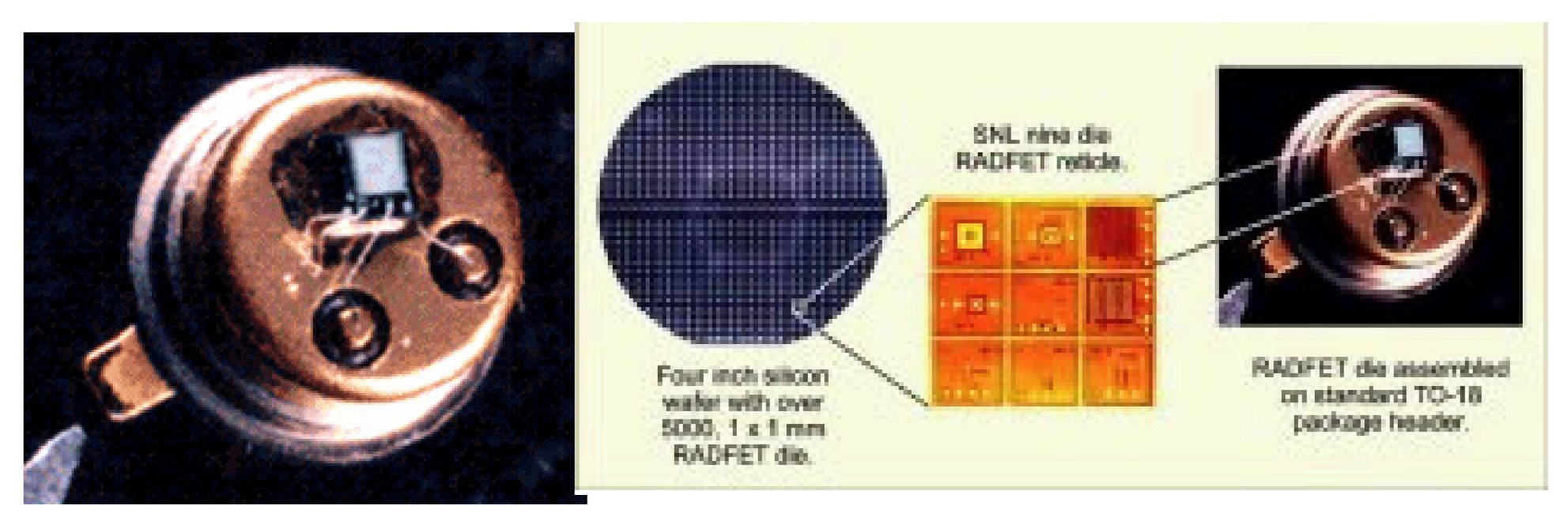
RadFET (Radiation field-effect transistor)
Cadmium zinc telluride (CZT) detectors
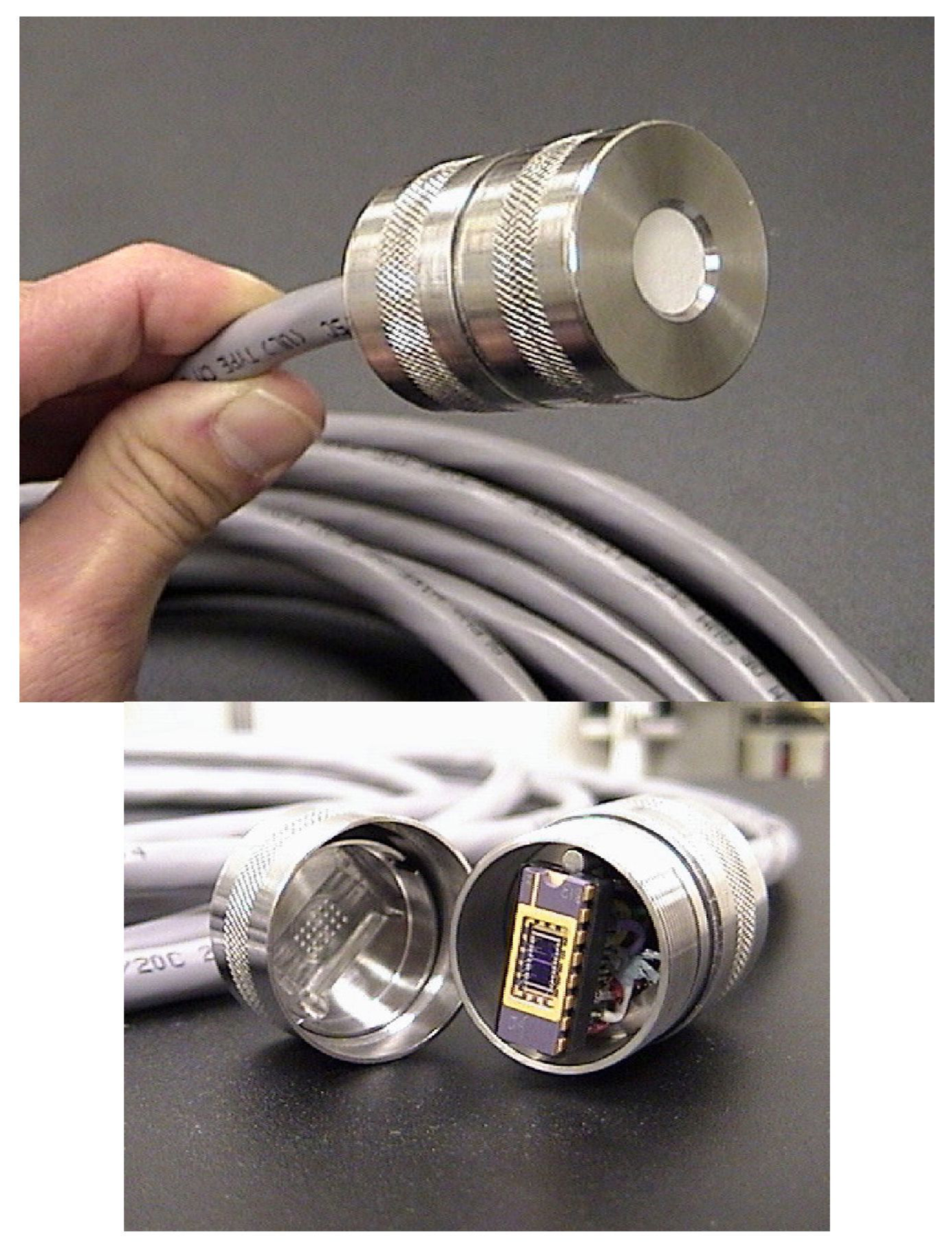
-Low-energy pin diodes beta spectrometer
-Thermoluminescent dosimeter (TLD)
-Isotope identification gamma detector
-Neutron generator for nuclear material detection
-Non-sandia radiation detectors
Volatile organic compound sensors
-Evanescent fiber-optic chemical sensor
-Grating light reflection spectroelectrochemistry
-Miniature chemical flow probe sensor
-SAW chemical sensor arrays
-MicroChemLab (gas phase)
-Gold nanoparticle chemiresistors
-Electrical impedance of tethered lipid bilayers on planar electrodes
-MicroHound
-Hyperspectral imaging
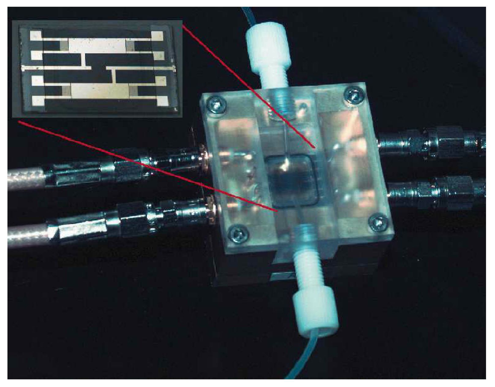
-Chemiresistor array
Biological sensors
-Fatty acid methyl esters (FAME) analyzer
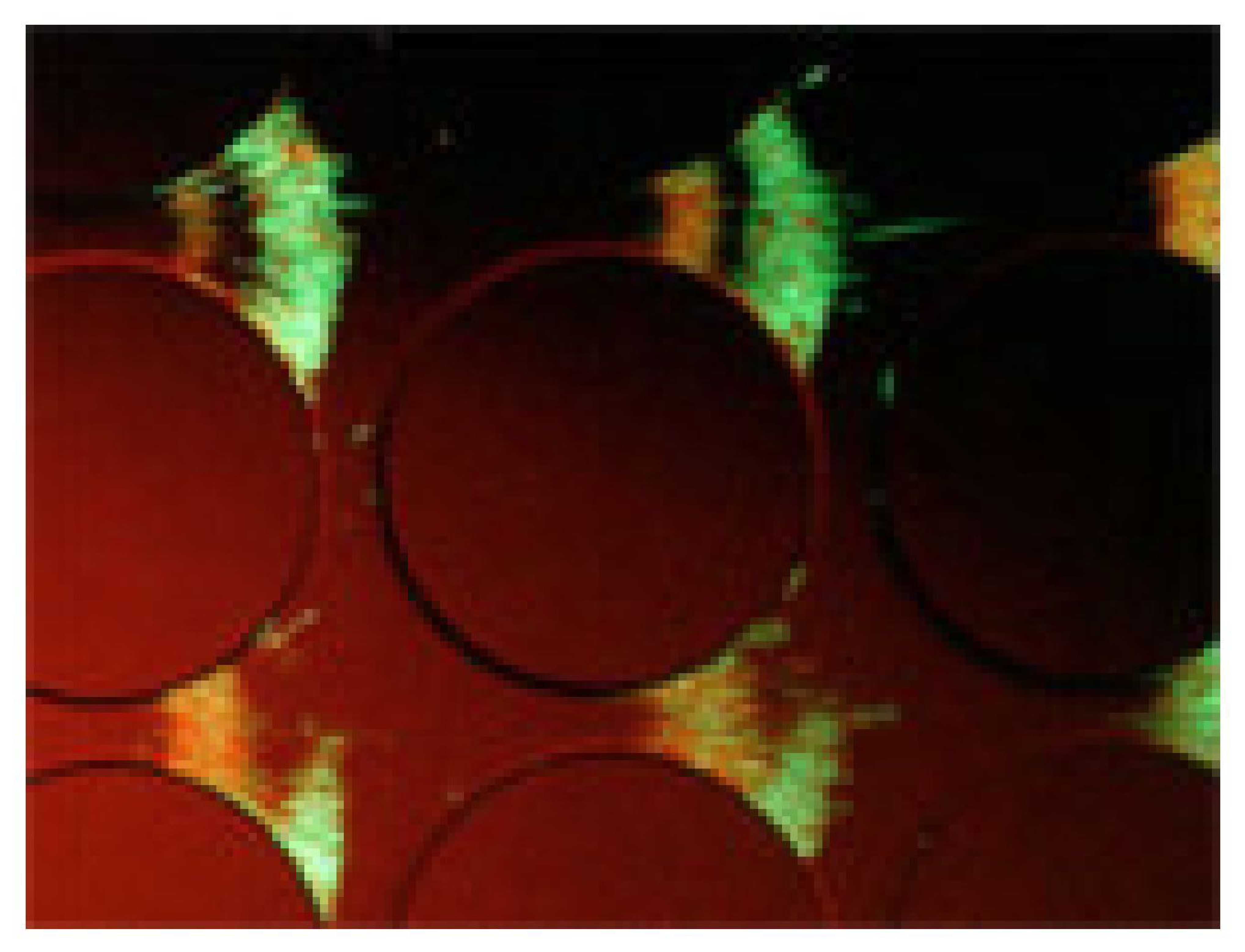
-iDEP (insulator-based dielectrophoresis)
-Bio-SAW sensor
-μProLab
-MicroChemLab (Liquid)
Summary and specifications of sensor technologies
Summary and recommendations
Acknowledgments
References
- Looney, B.; Falta, R.W. (Eds.) Vadose zone Science and Technology Solutions.; Battelle Press: Columbus, OH, 2000; p. 1540.
- Wilson, LG.; Everett, L.G.; Cullen, S.J. (Eds.) Handbook of Vadose Zone Characterization & Monitoring; CRC Press: Boca Raton, FL, 1995.
- U.S. DOE. Assessment of the 2000 and 2001 Environmental Management Industry Times They Are A-Changin'; Prepared for the U.S. Department of Energy Office of Environmental Management, Office of Science and Technology (EM-50). Prepared by YAHSGS L1c.: Richland, Wa, August 2002. [Google Scholar]
- Stetter, J. TES Workshop on Technology Needs as Part of a Conference on Analytical Chemistry and Applied Spectroscopy, Pittsburg, Pa; 2001.
- U.S. Department of Energy. From Cleanup to Stewardship, a Companion Report to Accelerating Cleanup: Paths to closure and Background Information to Support the Scoping Process Required for the 1998 PEIS Settlement Study.; U.S. Department of Energy, Office of Environmental Management, October 1999. [Google Scholar]
- U.S. Department of Energy (DOE). Market Study to Determine Needs and Present Usage of Chemical Sensor Systems for Environmental Analytical Applications.; Final Report Submitted to: Characterization, Monitoring and Sensing Technology Crossscutting Program, Department of Energy, Ames Laboratory, Iowa State University, Ames, IA 50011-3020 Prepared by: The Unimar Group, Ltd; 325 Market St., Alton, Il. 62002, May 1996. [Google Scholar]
- Inspector General (IG) Report. Departmental Position on the Office of Inspector General Report IG-0461. Groundwater Monitoring Activities at Department of Energy Facilities. To: Phillip L. Holbrook, Deputy Inspector General for Audit Services.
- 65 Federal Register 64746. Final Reissuance of National Pollutant Discharge Elimination System (NPDES) Storm Water Multi-Sector General Permit for Industrial Activities; Notice; October 30 2000. [Google Scholar]
- 40 CFR Part 403. General Pretreatment Regulations for Existing and New Sources of Pollution.; EPA: Washington, DC, 2000. [Google Scholar]
- 40 Code of Federal Regulations (CFR). Part 414, Section 111; Organic Chemicals, Plastics, and Synthetic Fibers.; EPA: Washington, DC, 2003. [Google Scholar]
- American Conference of Governmental Industrial Hygienists (ACGIH). Threshold Limit Values for Chemical Substances and Physical Agents and Biological Exposure Indices; ACGIH: Cincinnati, 2000. [Google Scholar]
- Horton, R.J. “Sensor development: Micro-analytical solutions for water monitoring applications”; SAND2003-2575P; Sandia National Laboratories: Albuquerque, NM, 2003. [Google Scholar]
- Ashby, C.I.H.; Kelly, M.J.; Yelton, W.G.; Pfeifer, K.B.; Muron, D.J.; Einfeld, W.; Siegal, M.P. Functionalized nanoelectrode arrays for in situ identification and quantification of regulated chemicals in water. LDRD Annual Report 2002, 364. [Google Scholar]
- Hahn, D.W.; Hencken, K.R.; Johnsen, H.A. Performance testing of a laser-induced breakdown spectroscopy (LIBS) based continuous metal emissions monitor at a pyrolytic waste treatment facility.; SAND97-8270; Sandi a National Laboratories: Albuquerque, NM, 1997. [Google Scholar]
- Matalucci, R.V.; Esparza-Baca, C.; Jimenez, R.D. Characterization, monitoring, and sensor technology catalogue.; SAND95-3062; Sandia National Laboratories: Albuquerque, NM, 1995. [Google Scholar]
- Blevins, L.G.; Shaddix, C.R.; Sickafoose, S.M.; Walsh, P. M. Laser-induced breakdown spectroscopy at high temperatures in industrial boilers and furnaces.; SAND2003-8151J; Sandia National Laboratories: Albuquerque, NM, 2003. [Google Scholar]
- Moreno, D.J.; Hughes, R.C.; Jenkins, M.W.; Drumm, C.R. A simple ionizing radiation spectrometer/dosimeter based on radiation sensing field effect transistors (RadFETs).; SAND97-0255C; Sandia National Laboratories: Albuquerque, NM, 1997. [Google Scholar]
- Murray, W.S.; Butterfield, K.B.; Baird, W. Automated radioisotope identification using fuzzy logic and portable CZT detectors.; LA-UR-00-4791 (LANL), 2000. [Google Scholar]
- Doyle, B.L.; Vizkelethy, G.; Walsh, D. Ion beam induced charge collection (IBICC) studies of cadmium zinc telluride (CZT) radiation detectors.; SAND99-0917C; Sandia National Laboratories: Albuquerque, NM, 1999. [Google Scholar]
- Wampler, W.R.; Doyle, B.L. Low-energy beta spectroscopy using pin diodes to monitor tritium surface contamination. Nuclear Instruments and Methods in Physics Research A 1994, 349, 473. [Google Scholar]
- Schwank, J.R.; et al. Common-source TLD and RADFET characterization of Co-60, Cs-137, and x-ray irradiation sources; SAND97-1440J; Sandia National Laboratories: Albuquerque, NM, 1997. [Google Scholar]
- Carlson, G.A.; Lorence, L.J., Jr.; Vehar, D.W. Particle size effect in CaF2: Mn-teflon TLD response at photon energies from 5 to 1250 KeV.; SAND89-1788J; Sandia National Laboratories: Albuquerque, NM, 1989. [Google Scholar]
- Garcia, N. Site hears latest news on four key R&D projects. In Sandia Lab News; Sandia National Laboratories: Albuquerque, NM, March 5 2004; Volume 56. [Google Scholar]
- Blair, D.S. Evaluation of an evanescent fiber optic chemical sensor for monitoring aqueous volatile organic compounds.; SAND97-0782; Sandia National Laboratories: Albuquerque, NM, 1997. [Google Scholar]
- Zaidi, S.; McNeil, J.R.; Kelly, M.J.; Sweatt, W.C.; Kemme, S.A.; Blair, D.S.; Brodsky, A.M.; Smith, S.A. Grating light reflection spectroelectrochemistry for detection of trace amounts of aromatic hydrocarbons in water; SAND2000-1018; Sandia National Laboratories: Albuquerque, NM, 2000. [Google Scholar]
- Ricco, A.; Xu, C.; Allred, R.; Crooks, R. SAW chemical sensor arrays using new thin-film materials.; SAND94-0241C; Sandia National Laboratories: Albuquerque, NM, 1994. [Google Scholar]
- Cernosek, R.W.; Frye, G.C.; Martin, S.J. Method and apparatus for phase and amplitude detection. U.S. Patent # 5763283 1994. [Google Scholar]
- Sandia National Laboratoris, “μChemLab” [online]. 9 December 2002. http://www-irn.sandia.gov/organization/mstc/organization/micro-analytical/chemlab.html.
- Linker, K.L.; Brusseau, C.A.; Mitchell, M.A.; Adkins, D.R.; Pfeifer, K.B.; Rumpf, A.N.; Rohde, S.B. “Portable explosives detection system: MicroHound.; SAND2003-2254C; Sandia National Laboratories: Albuquerque, NM, 2003. [Google Scholar]
- Koehler, F.W.; Haaland, D.M. Quantitative determination of 2D hyperspectral image data.; SAND99-2133A; Sandia National Laboratories: Albuquerque, NM, 1999. [Google Scholar]
- Timlin, J.A.; Haaland, D.M.; Sinclair, M.B. Hyperspectral imaging and multivariate data analysis for biological and biomedical applications.; SAND2003-3955A; Sandia National Laboratories: Albuquerque, NM, 2003. [Google Scholar]
- Ho, C.K.; McGrath, L.K.; Davis, C.E.; Thomas, M.L.; Wright, J.L.; Kooser, A.S.; Hughes, R.C. Chemiresistor microsensors for in-situ monitoring of volatile organic compounds: final LDRD report.; SAND2003-3410; Sandia National Laboratories: Albuquerque, NM, 2003. [Google Scholar]
- Hughes, R.C.; Casalnuovo, S.A.; Wessendorf, K.O.; Savignon, D.J.; Hietala, S.; Patel, S.V.; Heller, E.J. Integrated chemiresistor array for small sensor platforms. SPIE Proceedings Paper 4038-62, AeroSense 2000, Orlando, Florida; 2000; p. 519. [Google Scholar]
- Ho, C.K.; Hughes, R.C. In-Situ Chemiresistor sensor package for real-time detection of volatile organic compounds in soil and groundwater. Sensors 2002, 2, 23. [Google Scholar]
- Mowry, C.; Morgan, C.; Kottenstette, R.; Dulleck, G., Jr.; Manginell, R.; Wally, K.; Baca, Q.; Theisen, L.; Chambers, W.; Trudell, D. LDRD annual report; Sandia National Laboratories: Albuquerque, NM, 2002; p. 65. [Google Scholar]
- Simmons, B.A.; Cauley, T.H.; Charest, J.L. High-throughput insulative dielectrophoresis (iDEP) in bulk manufactured polypropylene.; SAND2003-8512P; Sandia National Laboratories: Albuquerque, NM, 2003. [Google Scholar]
- Brozik, S.M.; Branch, D.W.; Osbourn, G.C.; Morgan, C.H.; Sasaki, D.Y. LDRD annual report.; Sandia National Laboratories: Albuquerque, NM, 2002; p. 168. [Google Scholar]
- Napolitano, L.M.; Potter, K.S.; Hasselbrink, E.; Brinker, C.J.; Wheeler, D.R.; Brozik, S.M.; Sasaki, D.Y.; Shepodd, T.J.; Singh, A.K.; Burns, A.R.; Casalnuovo, S.A.; Kemme, S.A.; Loy, D.A.; Bunker, B.C.; Thompson, A.P.; Potter, B.G.; Schoeniger, J.S. LDRD annual report.; Sandia National Laboratories: Albuquerque, NM, 2002; p. 438. [Google Scholar]
- Nolan, P. Sandia National Laboratories annual report 2003-2004; Sandia National Laboratories: Albuquerque, NM, 2004; p. 47. [Google Scholar]


| Contaminant | Maximum Contaminant Level Goal (mg/L) | Maximum Contaminant Level (mg/L) |
|---|---|---|
| Cryptosporidium | zero | See footnote* |
| Giardia lamblia | zero | See footnote* |
| Heterotrophic plate count | n/a | See footnote* |
| Legionella | zero | See footnote* |
| Total Coliforms (including fecal coliform and E. Coli) | zero | 5.0%** |
| Turbidity | n/a | See footnote* |
| Viruses (enteric) | zero | See footnote* |
- Cryptosporidium (as of1/1/02 for systems serving >10,000 and 1/14/05 for systems serving <10,000) 99% removal.
- Giardia lamblia: 99.9% removal/inactivation.
- Viruses: 99.99% removal/inactivation.
- Legionella: No limit, but EPA believes that if Giardia and viruses are removed/inactivated, Legionella will also be controlled.
- Turbidity: At no time can turbidity (cloudiness of water) go above 5 nephelolometric turbidity units (NTU); systems that filter must ensure that the turbidity go no higher than 1 NTU (0.5 NTU for conventional or direct filtration) in at least 95% of the daily samples in any month. As of January 1, 2002, turbidity may never exceed 1 NTU, and must not exceed 0.3 NTU in 95% of daily samples in any month.
- HPC: No more than 500 bacterial colonies per milliliter.
- Long Term Enhanced Surface Water Treatment (Effective Date: January 14, 2005): Surface water systems or (GWUDI) systems serving fewer than 10,000 people must comply with the applicable Long Term 1 Enhanced Surface Water Treatment Rule provisions (e.g., turbidity standards, individual filter monitoring, Cryptosporidium removal requirements, updated watershed control requirements for unfiltered systems).
- Filter Backwash Recycling: The Filter Backwash Recycling Rule requires systems that recycle to return specific recycle flows through all processes of the system's existing conventional or direct filtration system or at an alternate location approved by the state.
| Contaminant | Maximum Contaminant Level Goal (mg/L) | Maximum Contaminant Level (mg/L) |
|---|---|---|
| Chloramines (as Cl2) | MRDLG=4* | MRDL=4.0** |
| Chlorine (as Cl2) | MRDLG=4* | MRDL=4.0** |
| Chlorine dioxide (as ClO2) | MRDLG=0.8* | MRDL=0.8** |
| Contaminant | Maximum Contaminant Level Goal (mg/L) | Maximum Contaminant Level (mg/L) |
|---|---|---|
| Chlorite | 0.8 | 1.0 |
| Haloacetic acids (HAA5) | n/a* | 0.060 |
| Total Trihalomethanes (TTHMs) | n/a* | .08 |
- Trihalomethanes: bromodichloromethane (zero); bromoform (zero); dibromochloromethane (0.06 mg/L). Chloroform is regulated with this group but has no MCLG.
- Haloacetic acids: dichloroacetic acid (zero); trichloroacetic acid (0.3 mg/L). Monochloroacetic acid, bromoacetic acid, and dibromoacetic acid are regulated with this group but have no MCLGs.
| Contaminant | Max. Contaminant Level Goal (mg/L) | Max. Contaminant Level (mg/L) |
|---|---|---|
| Antimony | 0.006 | 0.006 |
| Arsenic | 0* | 0.010 (as of 01/23/06) |
| Asbestos (fiber >10 micrometers) | 7 million fibers per liter | 7 million fibers per liter |
| Barium | 2 | 2 |
| Beryllium | 0.004 | 0.004 |
| Cadmium | 0.005 | 0.005 |
| Chromium (total) | 0.1 | 0.1 |
| Copper | 1.3 | Action Level=1.3** |
| Cyanide (as free cyanide) | 0.2 | 0.2 |
| Fluoride | 4.0 | 4.0 |
| Lead | zero | Action Level=1.3** |
| Mercury (inorganic) | 0.002 | 0.002 |
| Nitrate (measured as Nitrogen) | 10 | 10 |
| Nitrite (measured as Nitrogen) | 1 | 1 |
| Selenium | 0.05 | 0.05 |
| Thallium | 0.0005 | 0.002 |
| Contaminant | Max. Contaminant Level Goal (mg/L) | Max. Contaminant Level (mg/L) |
|---|---|---|
| Acrylamide | zero | Treatment Technology* |
| Alachlor | zero | 0.002 |
| Atrazine | 0.003 | 0.003 |
| Benzene | zero | 0.005 |
| Benzo(a)pyrene (PAHs) | zero | 0.0002 |
| Carbofuran | 0.04 | 0.04 |
| Carbon tetrachloride | zero | 0.005 |
| Chlordane | zero | 0.002 |
| Chlorobenzene | 0.1 | 0.1 |
| 2,4-D | 0.07 | 0.07 |
| Dalapon | 0.2 | 0.2 |
| 1,2-Dibromo-3-chloropropane(DBCP) | zero | 0.0002 |
| o-Dichlorobenzene | 0.6 | 0.6 |
| p-Dichlorobenzene | 0.075 | 0.075 |
| 1,2-Dichloroethane | zero | 0.005 |
| 1,1-Dichloroethylene | 0.007 | 0.007 |
| cis-1,2-Dichloroethylene | 0.07 | 0.07 |
| trans-1,2-Dichloroethylene | 0.1 | 0.1 |
| Dichloromethane | zero | 0.005 |
| 1,2-Dichloropropane | zero | 0.005 |
| Di(2-ethylhexyl) adipate | 0.4 | 0.4 |
| Di(2-ethylhexyl) phthalate | zero | 0.006 |
| Dinoseb | 0.007 | 0.007 |
| Dioxin (2,3,7,8-TCDD) | zero | 0.00000003 |
| Diquat | 0.02 | 0.02 |
| Endothall | 0.1 | 0.1 |
| Endrin | 0.002 | 0.002 |
| Epichlorohydrin | zero | Treatment Technology* |
| Ethylbenzene | 0.7 | 0.7 |
| Ethylene dibromide | zero | 0.00005 |
| Glyphosate | 0.7 | 0.7 |
| Heptachlor | zero | 0.0004 |
| Heptachlor epoxide | zero | 0.0002 |
| Hexachlorobenzene | zero | 0.001 |
| Hexachlorocyclopentadiene | 0.05 | 0.05 |
| Lindane | 0.0002 | 0.0002 |
| Methoxychlor | 0.04 | 0.04 |
| Oxamyl (Vydate) | 0.2 | 0.2 |
| Polychlorinated biphenyls (PCBs) | zero | 0.0005 |
| Pentachlorophenol | zero | 0.001 |
| Picloram | 0.5 | 0.5 |
| Simazine | 0.004 | 0.004 |
| Styrene | 0.1 | 0.1 |
| Tetrachloroethylene | zero | 0.005 |
| Toluene | 1 | 1 |
| Toxaphene | zero | 0.003 |
| 2,4,5-TP (Silvex) | 0.05 | 0.05 |
| 1,2,4-Trichlorobenzene | 0.07 | 0.07 |
| 1,1,1-Trichloroethane | 0.20 | 0.2 |
| 1,1,2-Trichloroethane | 0.003 | 0.005 |
| Trichloroethylene | zero | 0.005 |
| Vinyl chloride | zero | 0.002 |
| Xylenes (total) | 10 | 10 |
- Acrylamide = 0.05% dosed at 1 mg/L (or equivalent).
- Epichlorohydrin = 0.01 % dosed at 20 mg/L (or equivalent).
| Contaminant | Max. Contaminant Level Goal | Max. Contaminant Level |
|---|---|---|
| Alpha particles | zero | 15 picocuries per Liter (pCi/L) |
| Beta particles and photon emitters | zero | 4 millirems per year |
| Radium 226 and Radium 228 (combined) | zero | 5 pCi/L |
| Tritium | zero | 20,000 pCi/L |
| Uranium | zero | 30 ug/L (as of 12/08/03) |
| Environmental Protection Agency | ||
|---|---|---|
| Effluent characteristics | BAT effluent limitations and NSPS1 | |
| Maximum for any one day | Maximum for monthly average | |
| Anthracene......................................... | 47 | 18 |
| Benzene ........................................... | 134 | 57 |
| Benzo(a)anthracene ................................. | 47 | 19 |
| 3,4-Benzofluoranthene ............................... | 48 | 20 |
| Benzo(k)fluoranthene ................................ | 47 | 19 |
| Benzo(a)pyrene ...................................... | 48 | 20 |
| Bis(2-ethylhexyl) phthalate ......................... | 258 | 95 |
| Carbon Tetrachloride ................................ | 380 | 142 |
| Chlorobenzene ....................................... | 380 | 142 |
| Chloroethane ......................................... | 295 | 110 |
| Chloroform ........................................... | 325 | 111 |
| Chrysene .............................................. | 47 | 19 |
| Di-n-butyl phthalate .................................. | 43 | 20 |
| 1,2-Dichlorobenzene ................................... | 794 | 196 |
| 1,3-Dichlorobenzene ................................... | 380 | 142 |
| 1,4-Dichlorobenzene ................................... | 380 | 142 |
| 1,1-Dichlorobenzene ................................... | 59 | 22 |
| 1,2-Dichlorobenzene ................................... | 574 | 180 |
| 1,1-Dichlorobenzene ................................... | 60 | 22 |
| 1,2-trans-Dichloroethylene ............................ | 66 | 25 |
| 1,2-Dichlorobenzene .................................... | 794 | 196 |
| 1,3-Dichloropropylene .................................. | 794 | 196 |
| Diethyl phthalale ...................................... | 113 | 46 |
| 2,4-Dimethylphenol .................................... | 47 | 19 |
| Dimethyl phthalate .................................... | 47 | 19 |
| 4.6-Dinitro-o-cresol .................................. | 277 | 78 |
| 2,4-Dinitrophenol ..................................... | 4,291 | 1,207 |
| Ethybenzene ........................................... | 380 | 142 |
| Fluoranthene ......................................... | 54 | 22 |
| Fluorene ............................................. | 47 | 19 |
| Hexachlorobenzene ...................................... | 794 | 196 |
| Hexachlorobutadiene ................................... | 380 | 142 |
| Hexachloroethane ..................................... | 794 | 196 |
| Methyl Chloride ........................................ | 295 | 110 |
| Methylene Chloride ..................................... | 170 | 36 |
| Naphthalene ........................................... | 47 | 19 |
| Nitrobenzene ......................................... | 6,402 | 2,237 |
| 2-Nitrophenol ........................................ | 231 | 65 |
| 4-Nitrophenol .......................................... | 576 | 162 |
| Phenanthrene ........................................... | 47 | 19 |
| Phenol ............................................... | 47 | 19 |
| Pyrene .............................................. | 48 | 20 |
| Tetrachloroethylene .................................. | 164 | 52 |
| Toluene ............................................... | 74 | 28 |
| Total Chromium ........................................ | 2,770 | 1,110 |
| Total Copper .......................................... | 3,380 | 1,450 |
| Total Cyanide ......................................... | 1,200 | 420 |
| Total Lead ............................................ | 690 | 320 |
| Total Nickel ........................................... | 3,980 | 1,690 |
| Total Zinc2 .............................................. | 2,610 | 1,050 |
| 1,2,4-Trichlorobenzene .................................. | 794 | 196 |
| 1.1,1-Trichloroethene .................................... | 59 | 22 |
| 1,1,2-Trichloroethene ................................... | 127 | 32 |
| Trichloroethene ........................................ | 69 | 26 |
| Vinyl Chloride ......................................... | 172 | 97 |
| Hazardous Air Pollutant | Threshold Limit Value (ppm) | |
|---|---|---|
| 8-Hour Time Weighted Average | 15-Minute Short-Term Exposure Limit | |
| Benzene | 0.5 | 2.5 |
| Xylenes | 100 | 150 |
| Trichloroethylene | 50 | 100 |
| Pollutant | Goals | Enforceable Standards | ||
|---|---|---|---|---|
| Albuquerque | New Mexico State | Federal Primary | Federal Secondary | |
| Carbon Monoxide (CO) | ||||
| 8-hour average | --- | 8.7 ppm | 9.0 ppm | 9.0 ppm |
| 1-hour average | 13ppm | 13.1 ppm | 35 ppm | 35 ppm |
| Nitrogen Dioxide (NO2) | ||||
| 24-hour average | .062 ppm | 10 ppm | --- | --- |
| Annual arithmetic mean | .053 ppm | .05 ppm | .053ppm | .053 ppm |
| Ozone (O3) | ||||
| 1-hour average | .120 ppm | --- | .120 ppm | .120 ppm |
| Sulfur Dioxide (SO2) | ||||
| 24-hour average | .10 ppm | .10 ppm | --- | .140 ppm |
| 3-hour average | --- | --- | --- | .5 ppm |
| Annual arithmetic mean | .004 ppm | .02 ppm | .03 ppm | --- |
| Particulate Matter (PM10) | ||||
| 24-hour average | 150 μg/m3 | --- | 150μg/m3 | --- |
| Annual arithmetic mean | --- | --- | --- | 50 μg/m3 |
| Lead(Pb) | ||||
| Quarterly arithmetic mean | 1.5 μg/m3 | --- | 1.5 μg/m3 | 1.5 μg/m3 |
| Hydrogen Sulfide | ||||
| 1-hour average | .003 ppm | .010 ppm | --- | --- |
| Total Reduced Sulfur | ||||
| 1/2 hour average | --- | .003 ppm | --- | --- |
| 1-hour average | .003 ppm | --- | --- | --- |
| Particulate Matter (TSP) | ||||
| 24-hour average | 150 μg/m3 | 150 μg/m3 | --- | --- |
| 7-day average | --- | 110 μg/m3 | --- | --- |
| 30-day average | --- | 90 μg/m3 | --- | --- |
| Annual geometric mean | 60 μg/m3 | 60 μg/m3 | --- | --- |
| Sensor Technology | Specifications | |||||||
|---|---|---|---|---|---|---|---|---|
| Sensitivity | Selectivity | Stability | Speed | Size | Power | User Interface | Cost | |
| A) Nanoelectro de Array | low ppb | elemental in non-complex mixtures | long-term | seconds | 1 square inch dip probe | personal computer | sensor: | |
| B) Laser-Induced Breakdown Spectroscop y | low ppb | elemental | long-term | Ms with intensified-CCD, minutes with scanning spectrometers or signal averaging | fiber-optics; lengths of 100+ meters possible | mW per pulse | personal computer | system: $50-150K |
| Sensor Technology | Specifications | |||||||
|---|---|---|---|---|---|---|---|---|
| Sensitivity | Selectivity | Stability | Speed | Size | Power | User Interface | Cost | |
| A) RadFET | 5 mV/rad | speciation with filters | > 1 year, 5% drift over 1000 hours after strongexposure | milliseconds, or cumulative expose can be read later | ¼” with ASIC and dip | Passive ormW bias | sensitive digital multimeter | <$1 in volume |
| B) Cadmium Zinc Telluride detectors (CZT) | 0.8 mV/keV | very selective with spectroscopy | long-term | microseconds | 3mmˆ2 plus electronics | < 1 Watt | hand held or personal computer | $3000+ for system |
| C) Low-energy Pin Diodes Beta Spectrometer | single events > 1.4 keV. Above background noise, LODisO.1 disintegrations/cmA2/sec(3 rem/year) | very selective | long-term | 20 ms | sensor: 13 mm2, plus electronics | Passive or mW bias | hand held or personal computer | $1000+ for photodiode |
| D) Thermoluminescent Dosimeter (TLD) | 1 micro-rad/hour | non-specific to radiation source, but can employ filters or different crystal thicknesses and types | long-term | cumulative dose; nanoseconds per event | 5mmˆ2 | passive | TLD Reader | low dollars for crystals; $1000+ for reader |
| E) Isotope Identification Gamma Detector | very high | very selective | long term | seconds | vehicle portal | 110 AC | laptop | |
| F) Neutron Generator for Nuclear Material Detection | very high | very selective | long term | seconds | 1 meter tall | 110 AC | laptop | |
| Sensor Technology | Specifications | |||||||
|---|---|---|---|---|---|---|---|---|
| Sensitivity | Selectivity | Stability | Speed | Size | Power | User Interface | Cost | |
| A) Fiber Optic Chemical Sensor | low ppm for hydrophobic organics | good selectivity with multivariate analysis in moderately complex environments; coating is nonspecific for hydrophobic compounds | weekly calibration | 20 minutes | fiber-optics; lengths up to kilometers possible | 110 V, 5 amps | laptop | $0.25/meter $2500 for spectrometer |
| B) Grating Light Reflection Spectro-electrochemistry | ppm to ppb | multivariate analysis required for simple mixtures | long term | seconds to minutes | dip probe | 5 Watts | laptop | <$500 |
| C) Miniature Chemical Flow Probe Sensor | Lowppbtolow ppm, depending on analyte | good selectivity in moderately complex matrix | flow cell and fresh reagents ensure high reproducibility | 1-2 minutes | 2″ probe diameter, up to 150 feet long; spectrometer andPC in 2 suitcases | 110 AC when built (1995) | laptop | $10K for total system |
| D) SAW Chemical Sensor Arrays | ppm to ppb | good with multivariate analysis of mixtures that are not too complex | slow drift over time | tens of seconds | < 1 square inch sensor | mW | laptop or digital display | <$500 |
| E) MicroChemLab (gas phase) | ppb | very good | slow drift over time | 1-5 minutes | handheld | < 1 Watt | laptop or digital display | $10-20K |
| F) Gold Nanoparticle Chemiresistors | ppb | may be tailored to chemical classes | TBD | seconds | < 1 square inch sensor | mW | laptop or digital display | <$100 |
| G) Electrical Impedance of Tethered Lipid Bilayerson Planar Electrodes | ppm to ppb | very high with antibody coatings; lower for non-specific receptors | weeks | minutes | cm^2 | mW for sensor; 110 AC for whole instrument | laptop | <$1 per sensor |
| H) MicroHound | ppb | fairly high | days to weeks | seconds | handheld | battery | laptop or digital display | <$5K |
| 1) Hyperspectral Imaging | ppm to ppb | good with multivariate analysis of mixtures that are not too complex | long term | seconds to minutes | handheld | laptop | $10K to $100K | |
| J) Chemiresistor Arrays | ∼typically tens to hundreds of ppm;0.1% of saturatedvapor pressure | arrays can discriminate different classes of VOCs | slow drift over time | seconds to minutes, depending onconcentration | several mm; package is ∼2.5 cm diameter x∼6 cmlong | mW; battery powered | laptop or computer | <$100 for sensor array; package can be ∼$500 |
| Sensor Technology | Specifications | |||||||
|---|---|---|---|---|---|---|---|---|
| Sensitivity | Selectivity | Stability | Speed | Size | Power | User Interface | Cost | |
| A) Fatty Acid Methyl Esters (FAME) Analyzer | low nanograms | highly selective | SAW sensor can irreversibly load | < 10 min. | handheld | < 5 Watts per analysis | syringe and keypad or laptop | potentially <$10K |
| B) iDEP (insulator-based dielectrophoresis) | Preconcentration method for other sensors | non-selective | expected to be high | milliseconds | millimeters | < 1 W | Is a module for larger systems | <$1 |
| C) Bio-SAW Sensor | picograms of proteins | highly selective | SAW can drift overtime; analyte binding can be irreversible | minutes | several square cm | mW | system display plus some liquid handling; laptop | <$100 per sensor |
| D) μProLab | picograms | expected to be highly selective | acoustic sensors tend to drift with time; optical systems will be more stable | minutes | handheld | <5 W | minimal fluid handling, system display or laptop | TBD |
| E) MicroChemLab (Liquid) | depending on analyte: 10-100 ppbfor chemicals; sub-toxic(picomoles)forbiotoxins | very high | hours | <5 min | handheld | 5 Watts | LCD display or laptop | <$10K |
| Requirements | Drinking Water | Storm Water | Pre-Treatment | Ambient Air |
|---|---|---|---|---|
| Concentration | Lowest concentrations (ppb to ppm in aqueous phase) | Higher concentrations than drinking water (e.g., arsenic is 160 ppb in storm water for wood preservers while drinking water is 10 ppb) | Concentration are higher than drinking water (e.g., TCE is 69 ppb (daily) compared to 5 ppb for drinking water); almost all biological except for a few industries that manufacture chemicals; INDUSTRY SPECIFIC | Air concentrations are typically in the ppm range |
| Sampling Frequency | Most frequent sampling of the three water applications (would like real time, continuous monitoring) | Only need to sample occasionally (during rain storms) | More frequent monitoring than for storm water but less than for drinking water | Continuous (current methods average over a period of time using continuous flow) |
| Sampling Method | On-line, continuous with remote telemetry | Can be hand-held for occasional sampling | On-line or hand-held | Continuous air monitoring with remote telemetry |
| Sample Phase | Aqueous | Aqueous | Aqueous | Gas |
| Sensor Technology | Application | Analyte | Comments |
|---|---|---|---|
| LIBS | Drinking Water, Storm Water, Pretreatment | Trace Metals | The cost of the laser and spectrometer are high. Additional development needs to bring the price down and package it for use in water applications. Could potentially be used to simultaneously identify 9 RCRA metals plus arsenic. Sampling interval ranges from 1 s to ∼1 minute (for signal averaging). Can be run continuously. |
| Nanoelectrode Array | Drinking Water, Storm Water, Pretreatment | Trace Metals | Less selective than LIBS. Commercial company in Washington. Sampling interval on the order of seconds. Still under development to discern among multiple target analytes present. |
| Miniature Chemical Flow Probe Sensor | Drinking Water, Storm Water, Pretreatment | VOCs, Trace Metals | Expensive because of spectrometry (like LIBS). Reagents need to be supplied. Need to acquire sample to introduce reagent in a side-stream. |
| RadFET | Drinking Water | Radioisotopes | Need to use filters to allow speciation. Sensitivity in water for alpha and beta emitters is questionable given the attenuation through water. |
| Low-energy Pin Diodes Beta Spectrometer | Drinking Water | Radioisotopes | Commercially available. May not need any additional development. Sensitivity in water for alpha and beta emitters is questionable given the attenuation through water. |
| Cadmium Zinc Telluride Detectors | Drinking Water | Radioisotopes | Commercially available. Sensitivity in water for alpha and beta emitters is questionable given the attenuation through water. |
| SAWs | Drinking Water, Storm Water, Pretreatment, Air | VOCs | Sensitivity can get down to ∼ppm, but fluctuations in environmental parameters (e.g., humidity, temperature) can reduce the sensitivity and accuracy. Sensor signal drifts over time. Cannot analyze more than three contaminants at once. |
| Chemiresistors | Drinking Water, Storm Water, Pretreatment, Air | VOCs | Sensitivity is limited (hundreds of ppm). Needs preconcentration. These can also be used to monitor in-situ remediation activities (patent pending: SD-7097 Automated Monitoring and Remediation System for Volatile Subsurface Contaminants). |
| MicroHound/lon Mobility Spectrometer (IMS) | Drinking Water, Storm Water, Pretreatment, Air | Semi-Volatile Organic Compounds | Gas-phase detection; need to develop a sampling system to introduce water samples to IMS. Should be able to detect semi-volatile chlorinated hydrocarbons (e.g., polychlorinated biphenyls (PCBs)). Can detect pesticides, organic nitrates. |
| MicroChemLab (gas) | Drinking Water, Storm Water, Pretreatment, Air | VOCs | MCL is manufacturing these for ∼$10K per unit. Additional development work is needed to adapt these systems for VOCs. |
| MicroChemLab (liquid) | Drinking Water | Biological | Cost is high. |
| FAME | Drinking Water | Biological | Sampling is currently done manually. |
| Sensor | Analyte | Future Development Required |
|---|---|---|
| LIBS | Trace Metals | LIBS systems employ diffraction gratings that must be scanned to cover the spectral range of metal contaminants with sufficient resolution for positive identification and quantification. Speed could be increased through the use of Sandia's programmable diffraction grating. Simultaneous determination could be made through the computer-aided design of holographic diffraction gratings. |
| CZT | Radioisotopes | These detectors are inexpensive and sensitive to regulated radiation levels. Commercial spectrometer systems are available. A low level effort could adapt the spectrometer for water monitoring. Alpha emitting contaminants in water can not be detected by radiation events as alpha radiation is nonpenetrating. |
| MicroChemLab, gas phase | VOCs | Due to the wide variety of organic contaminants that can be present in air or water, separation is essential for analysis. The MicroChemLab can be adapted to collect and analyze in both air and water. Leveraging funding could direct development towards specific targets. |
| MicroHound/lon Mobility Specrometry | Semi-Volatiles | The ion mobility spectrometer behind this instrument can be used in positive mode for common semi-volatiles or negative mode for highly selective detection of pesticides and halogenated semivolatiles. The diffusion-based separation could benefit from a pre-separation using a chromatography column. |
| Bio-SAW Sensor | Biological Pathogens | Sensors with bioreceptors are highly selective, providing detection amplification over background contaminants. Still, biofouling can occur. Further development is needed to array significant numbers of sensors into a small area for multi-pathogen monitoring. |
© 2005 by MDPI ( http://www.mdpi.org). Reproduction is permitted for non-commercial purposes.
Share and Cite
Ho, C.K.; Robinson, A.; Miller, D.R.; Davis, M.J. Overview of Sensors and Needs for Environmental Monitoring. Sensors 2005, 5, 4-37. https://doi.org/10.3390/s5010004
Ho CK, Robinson A, Miller DR, Davis MJ. Overview of Sensors and Needs for Environmental Monitoring. Sensors. 2005; 5(1):4-37. https://doi.org/10.3390/s5010004
Chicago/Turabian StyleHo, Clifford K., Alex Robinson, David R. Miller, and Mary J. Davis. 2005. "Overview of Sensors and Needs for Environmental Monitoring" Sensors 5, no. 1: 4-37. https://doi.org/10.3390/s5010004
APA StyleHo, C. K., Robinson, A., Miller, D. R., & Davis, M. J. (2005). Overview of Sensors and Needs for Environmental Monitoring. Sensors, 5(1), 4-37. https://doi.org/10.3390/s5010004