
Rotary 3D Magnetic Field Scanner for the Research and Minimization of the Magnetic Field of UUV


Abstract
:1. Introduction
- Measurement using special infrastructure on land: only the magnetic field (and partial airborne equipment acoustic testing [2]), as the other fields require the presence of a water medium;
2. Description of the Test Stand
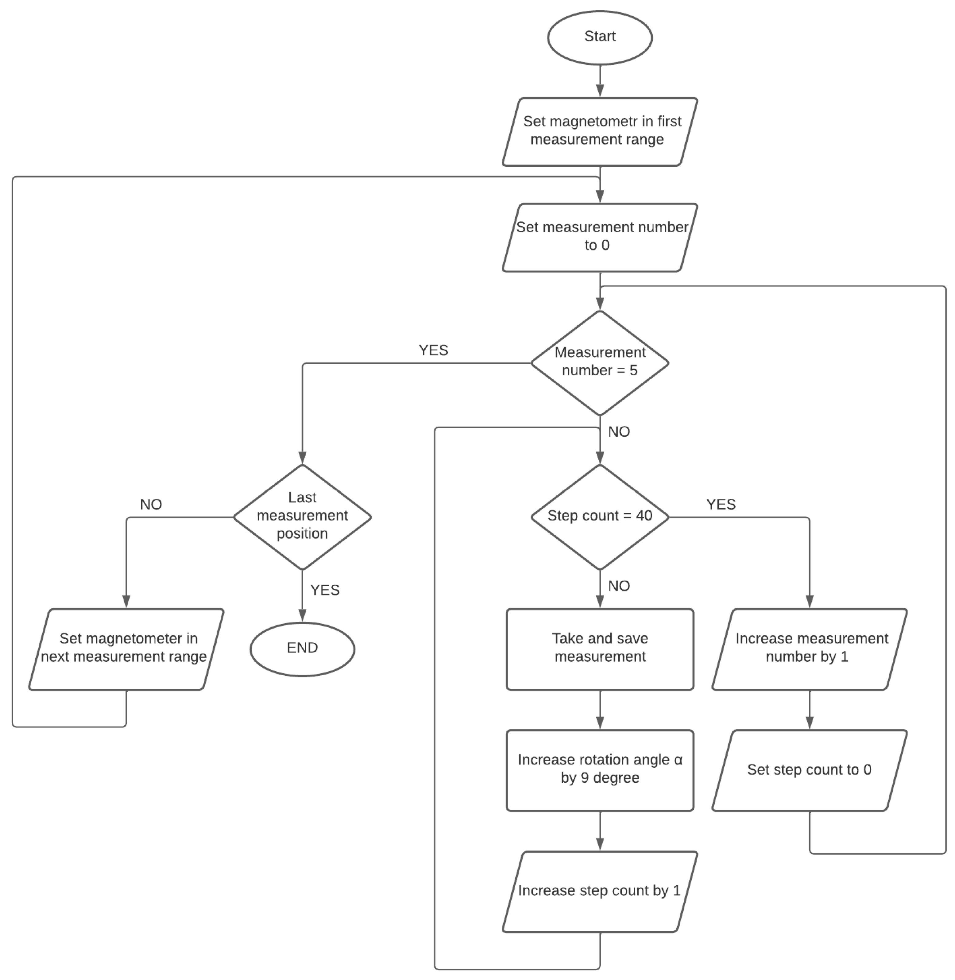
3. Research Methods
4. Calculation Method
- is the value of the X-axis component of the sensor;
- is the value of the Y-axis component of the sensor; and
- is the value of the Z-axis component of the sensor.
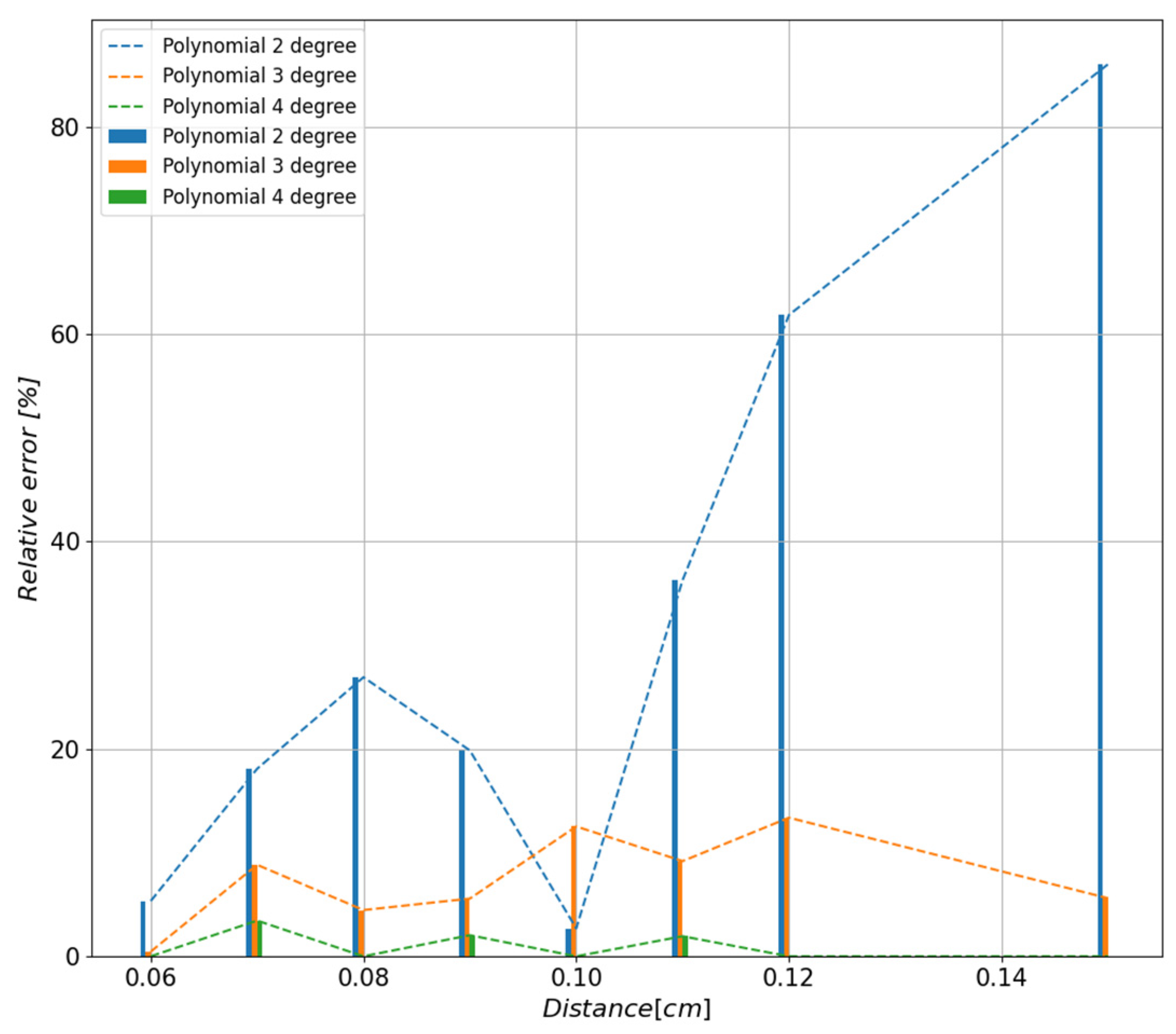
4.1. Study of the Influence of the Degree of the Approximating Polynomial on the Quality of the Obtained Results
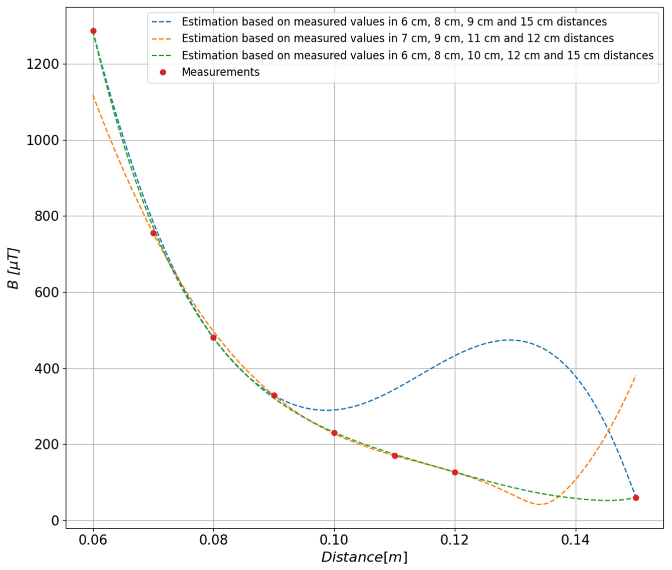
4.2. Study of the Impact of Data Selection on the Quality of the Approximating Polynomial
5. Results
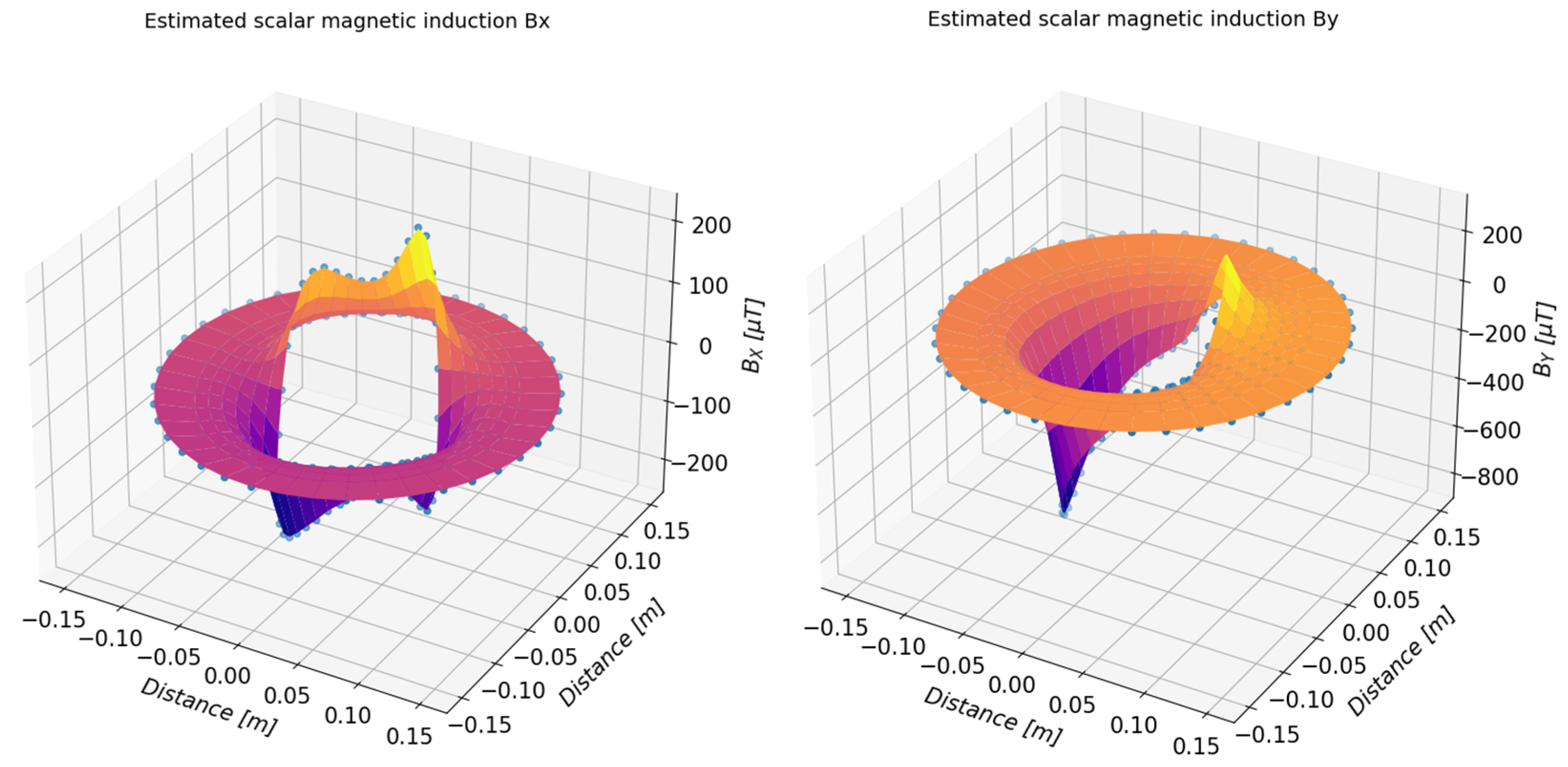
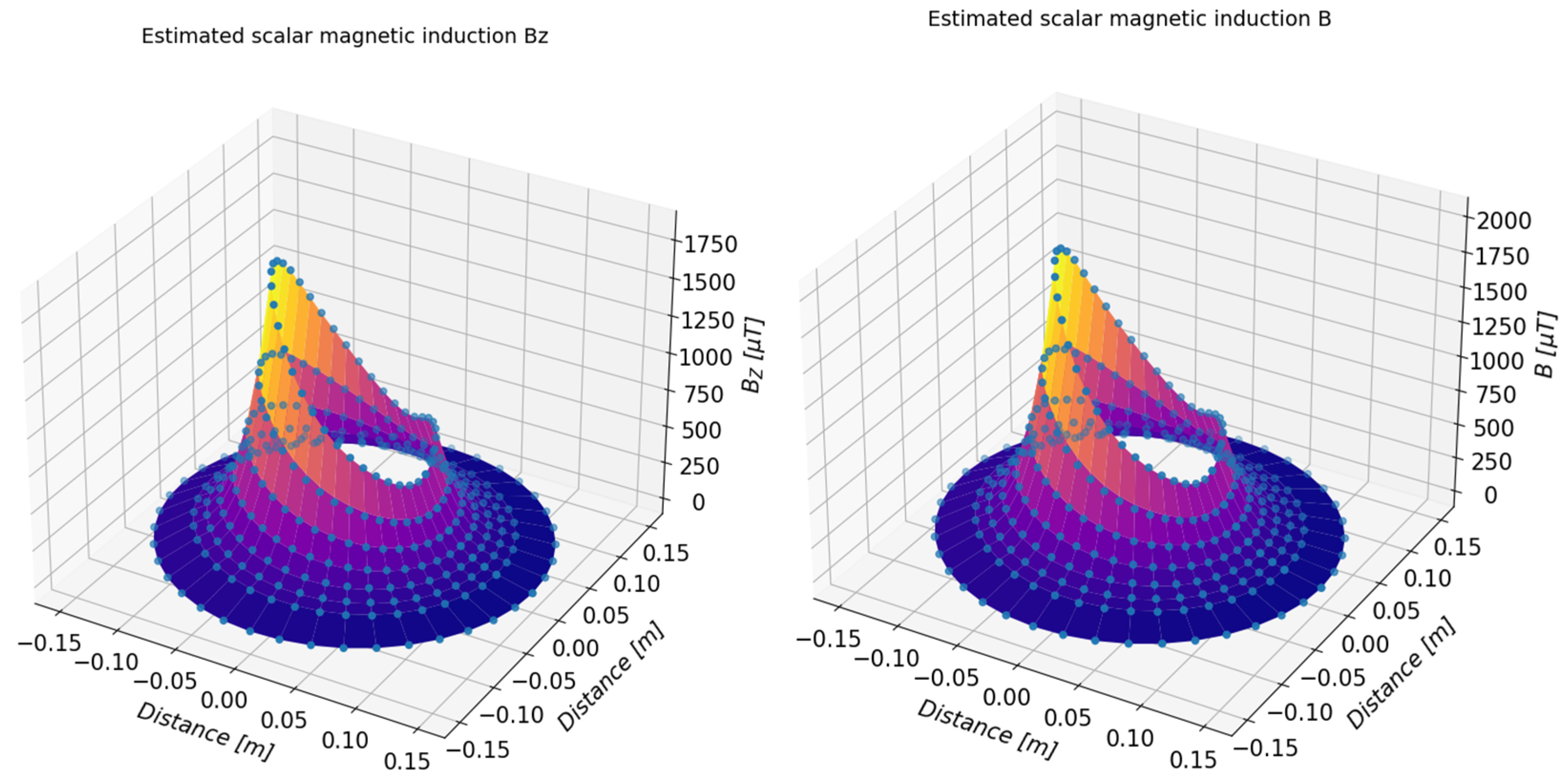
5.1. Study of the Toroidal Magnet
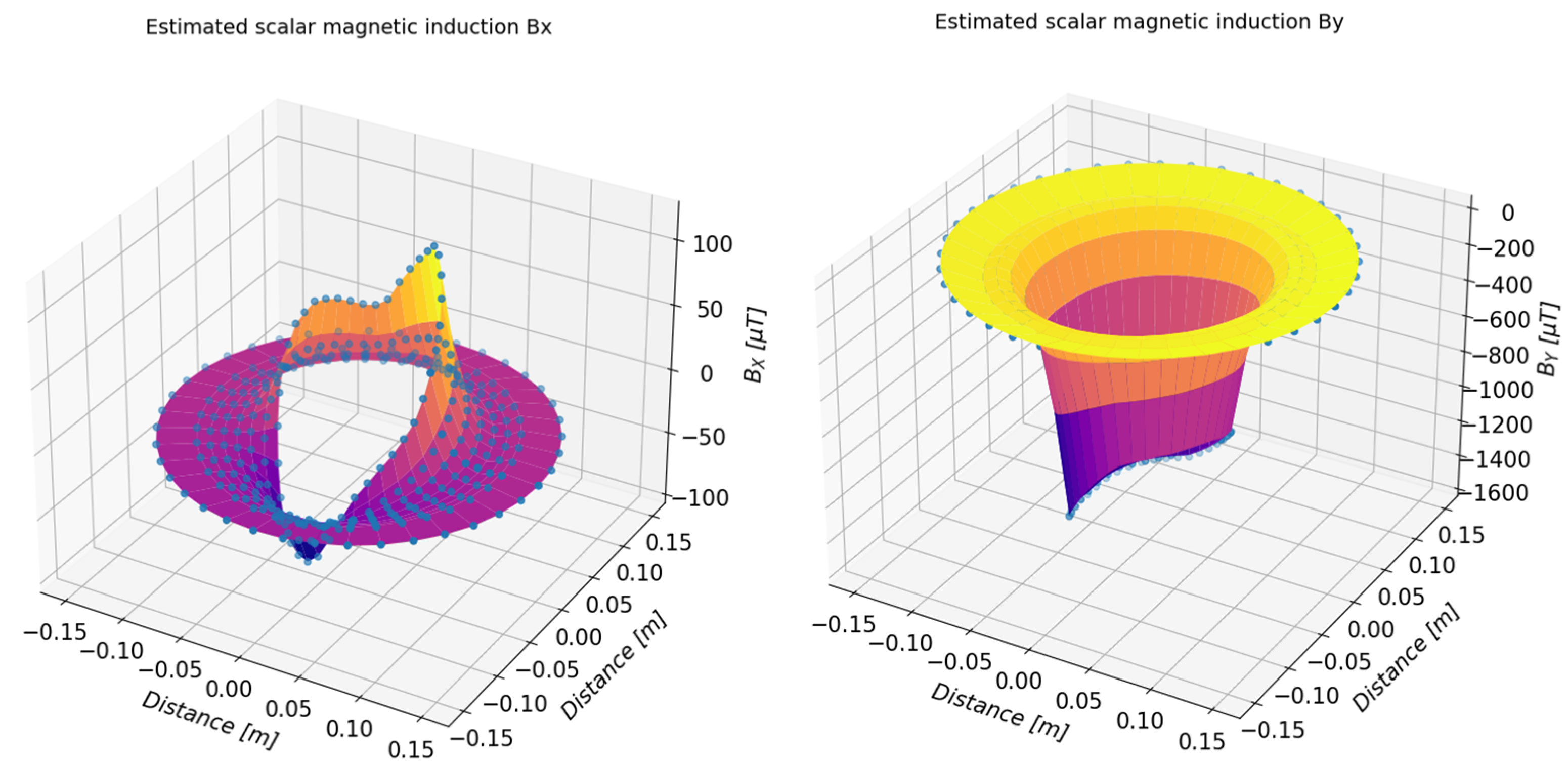
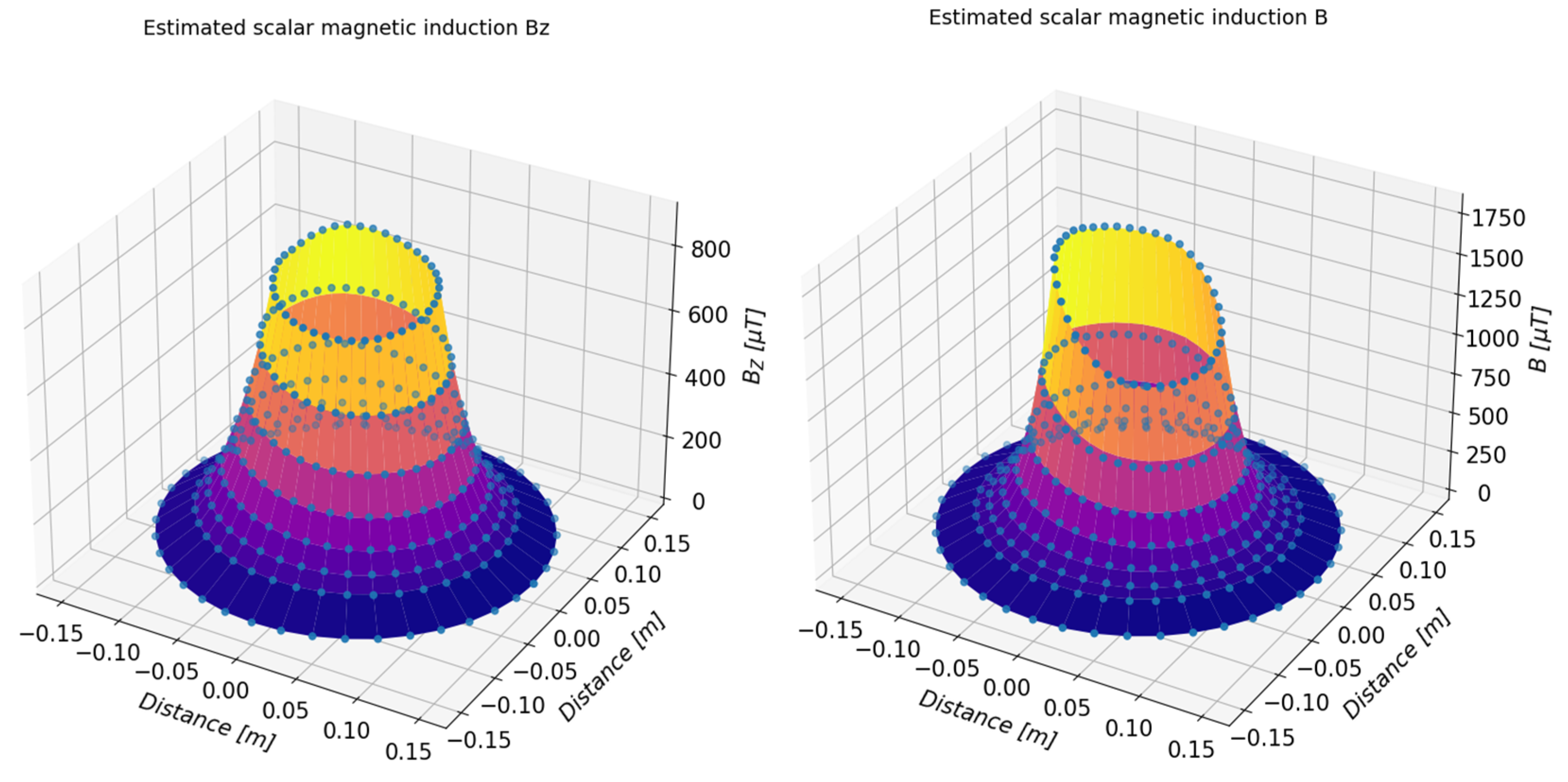
5.2. Study of a Group of Magnets Arranged in Irregular Form
6. Conclusions
Author Contributions
Funding
Institutional Review Board Statement
Informed Consent Statement
Data Availability Statement
Conflicts of Interest
References
- NATO STANAG—1364; Standard Magnetic and Acoustic Criteria for Reusable MCM Underwater Vehicles, Revision 3—Classified. 18 January 2010. Available online: https://publishers.standardstech.com/stgnet#information5A715085 (accessed on 31 October 2022).
- Grzeczka, G.; Listewnik, K.; Kłaczyński, M.; Cioch, W. Examination of the vibroacoustic characteristics of 6 kW proton exchange membrane fuel cell. J. Vibroeng. 2015, 17, 4025–4034. [Google Scholar]
- Armstrong, B.; Pentzer, J.; Odell, D.; Bean, T.; Canning, J.; Pugsley, D.; Frenzel, J.; Anderson, M.; Edwards, D. Field Measurement of Surface Ship Magnetic Signature Using Multiple AUVs. Defence Technical Information Center. Available online: https://apps.dtic.mil/sti/pdfs/ADA516664.pdf (accessed on 12 December 2022).
- Listewnik, K. Sound Silencing Problem of Underwater Vehicles. Solid State Phenom. 2013, 196, 212–219. [Google Scholar] [CrossRef]
- Elliott, K.C.; Montgomery, R.; Resnik, D.B.; Goodwin, R.; Mudumba, T.; Booth, J.; Whyte, K. Drone Use for Environmental Research [Perspectives]. IEEE Trans. Geosci. Remote Sens. 2019, 7, 106–111. [Google Scholar] [CrossRef]
- Norgren, P.; Lubbad, R.; Skjetne, R. Unmanned Underwater Vehicles in Arctic Operations. In Proceedings of the 22nd IAHR International Symposium on Ice, Singapore, 11–15 August 2014. [Google Scholar]
- Bauer, K. Clearance of Contaminated Sites in the Sea. Available online: https://www.munitect.de/sites/all/download/Munitectpaper.pdf (accessed on 12 December 2022).
- Boatman, M. Environmental Studies of the Electromagnetic Fields (EMF) & Marine Life. Available online: https://www.boem.gov/sites/default/files/documents/renewable-energy/state-activities/Electromagnetic-Fields-Marine-Life.pdf (accessed on 12 December 2022).
- Hall, E.T. Use of Proton Magnetometer in Underwater Archaeology. Archaeometry 2007, 9, 32–43. [Google Scholar] [CrossRef]
- Balestrieri, E.; Daponte, P.; De Vito, L.; Lamonaca, F. Sensors and Measurements for Unmanned Systems: An Overview. Sensors 2021, 21, 1518. [Google Scholar] [CrossRef] [PubMed]
- Marwan, N.; Schwarz, U.; Kurths, J. The Earth magnetic field in the last 100 kyr. In Proceedings of the Conference of the DFG Priority Programme 1097, Nice, France, 6–11 April 2003. [Google Scholar]
- Matsuoka, A.; Matsumura, K.; Kubota, A.; Tashiro, K.; Wakiwaka, H. Residual magnetization measurements of a motor to be used in satellites. In Proceedings of the SPIE 7500—The International Society for Optical Engineering, Gwangju, Republic of Korea, 3–5 December 2009. [Google Scholar]
- Listewnik, K.; Grzeczka, G.; Kłaczyński, M.; Cioch, W. An on-line diagnostics application for evaluation of machine vibration based on standard ISO 10816-1. J. Vibroeng. 2015, 17, 4248–4258. [Google Scholar]
- Gloza, I.; Buszman, K.; Listewnik, K. The passive module for underwater environment monitoring. In Proceedings of the 11th European Conference on Underwater Acoustics, Edinburgh, UK, 2–6 July 2012; pp. 1787–1793. [Google Scholar]
- Mouser Electronics. Digital Output Magnetic Sensor: Ultra-Low-Power, High-Performance 3-Axis Magnetometer. Available online: https://www.mouser.pl/datasheet/2/389/dm00075867-1797759.pdf (accessed on 31 October 2022).
- Freescale Semiconductor, Inc. How to Increase the Analog-to-Digital Converter Accuracy in an Application. Available online: https://www.nxp.com/docs/en/application-note/AN5250.pdf (accessed on 31 October 2022).
- The Engineering ToolBox LK-12. Available online: https://www.engineeringtoolbox.com/permeability-d_1923.html (accessed on 31 October 2022).
- Enes Magnesy Paweł Zientek SP. K. Available online: https://magnesy.pl/magnesy-ferrytowe (accessed on 31 October 2022).
- Towards Data Science. Available online: https://towardsdatascience.com/polynomial-regression-bbe8b9d97491 (accessed on 31 October 2022).
- NumPY. Available online: https://numpy.org/doc/stable/reference/generated/numpy.polyfit.html (accessed on 31 October 2022).


| Symbol of the Material | Remanence BR [mT] | Coercive Field HC [kA/m] | Energy Density BHmax [kj/m3] | Curie Temperature TC [°C] |
|---|---|---|---|---|
| F10 (isotropic) | 200–235 | 210–280 | 6.5–9.5 | 450 |
| F20 | 320–380 | 140–195 | 18.0–22.0 | 450 |
| F25 | 360–400 | 140–200 | 22.5–28.0 | 450 |
| F30 | 370–400 | 180–220 | 26.0–30.0 | 450 |
| F30BH | 380–400 | 235–290 | 27.0–32.5 | 450 |
| F35 | 410–430 | 225–255 | 31.5–35.0 | 450 |
| Measurement Distance r [m] | 0.06 | 0.07 | 0.08 | 0.09 | 0.10 | 0.11 | 0.12 | 0.15 |
| Total Magnetic Induction B [µT] | 781 | 462 | 300 | 206 | 145 | 106 | 75 | 24 |
| Rotation Angle [°] | Estimated Magnetic Induction Values of Component Bx [µT] as a Function of Rotation Angle and Measurement Distance | |||||||
|---|---|---|---|---|---|---|---|---|
| 6.0 cm | 7.0 cm | 8.0 cm | 9.0 cm | 10.0 cm | 11.0 cm | 12.0 cm | 15.0 cm | |
| 0 | 45.05 | 12.53 | −7.47 | −17.56 | −20.37 | −18.49 | −14.57 | −16.58 |
| 9 | 57.68 | 20.25 | −3.03 | −15.09 | −18.87 | −17.31 | −13.35 | −16.49 |
| 18 | 71.49 | 29.06 | 2.32 | −11.94 | −16.93 | −15.88 | −12.0 | −15.61 |
| 27 | 86.95 | 37.87 | 6.79 | −9.97 | −16.07 | −15.19 | −10.99 | −15.21 |
| 36 | 99.79 | 44.93 | 10.21 | −8.51 | −15.32 | −14.36 | −9.74 | −15.11 |
| 45 | 110.3 | 51.36 | 13.86 | −6.57 | −14.28 | −13.64 | −9.01 | −14.81 |
| 54 | 112.87 | 53.47 | 15.64 | −5.01 | −12.88 | −12.38 | −7.91 | −14.7 |
| 63 | 105.12 | 50.56 | 15.38 | −4.3 | −12.38 | −12.73 | −9.27 | −14.81 |
| 72 | 95.84 | 45.41 | 13.03 | −4.95 | −12.17 | −12.28 | −8.93 | −14.55 |
| 81 | 85.14 | 40.33 | 11.4 | −4.83 | −11.56 | −11.99 | −9.3 | −14.48 |
| 90 | 72.65 | 34.44 | 9.56 | −4.63 | −10.81 | −11.6 | −9.67 | −14.06 |
| 99 | 57.65 | 27.16 | 6.94 | −5.01 | −10.66 | −12.02 | −11.07 | −14.25 |
| 108 | 52.09 | 23.82 | 5.14 | −5.83 | −10.94 | −12.08 | −11.12 | −14.38 |
| 117 | 52.15 | 23.55 | 4.72 | −6.26 | −11.29 | −12.28 | −11.15 | −14.15 |
| 126 | 54.67 | 24.78 | 5.13 | −6.28 | −11.46 | −12.43 | −11.19 | −14.37 |
| 135 | 57.38 | 25.88 | 5.31 | −6.5 | −11.7 | −12.47 | −10.96 | −14.41 |
| 144 | 58.6 | 26.81 | 5.98 | −6.05 | −11.43 | −12.33 | −10.92 | −14.42 |
| 153 | 58.91 | 26.93 | 6.05 | −5.93 | −11.22 | −12.03 | −10.58 | −14.69 |
| 162 | 53.35 | 23.94 | 4.66 | −6.48 | −11.5 | −12.39 | −11.14 | −14.59 |
| 171 | 48.08 | 20.43 | 2.45 | −7.77 | −12.19 | −12.71 | −11.29 | −14.63 |
| 180 | 36.18 | 13.65 | −1.02 | −9.38 | −13.01 | −13.47 | −12.33 | −14.99 |
| 189 | 23.76 | 5.75 | −5.72 | −12.01 | −14.44 | −14.34 | −13.06 | −15.44 |
| 198 | 8.13 | −3.52 | −10.86 | −14.78 | −16.15 | −15.85 | −14.76 | −15.6 |
| 207 | −12.58 | −15.86 | −17.52 | −17.94 | −17.5 | −16.6 | −15.62 | −16.05 |
| 216 | −36.55 | −30.15 | −25.34 | −21.9 | −19.57 | −18.15 | −17.38 | −16.73 |
| 225 | −58.51 | −43.54 | −32.95 | −26.0 | −21.9 | −19.89 | −19.2 | −17.35 |
| 234 | −74.63 | −54.21 | −39.76 | −30.23 | −24.56 | −21.73 | −20.66 | −17.68 |
| 243 | −84.68 | −61.64 | −45.15 | −34.08 | −27.32 | −23.72 | −22.15 | −18.38 |
| 252 | −90.1 | −66.32 | −49.04 | −37.19 | −29.67 | −25.4 | −23.27 | −18.86 |
| 261 | −91.65 | −67.98 | −50.66 | −38.65 | −30.88 | −26.32 | −23.9 | −18.99 |
| 270 | −84.58 | −64.9 | −50.04 | −39.25 | −31.82 | −27.02 | −24.11 | −19.44 |
| 279 | −69.15 | −57.01 | −46.94 | −38.78 | −32.34 | −27.45 | −23.94 | −19.85 |
| 288 | −50.01 | −46.95 | −42.7 | −37.72 | −32.51 | −27.54 | −23.29 | −19.67 |
| 297 | −34.17 | −37.95 | −38.19 | −35.83 | −31.81 | −27.08 | −22.57 | −19.8 |
| 306 | −23.29 | −31.34 | −34.47 | −33.87 | −30.76 | −26.33 | −21.79 | −19.49 |
| 315 | −12.35 | −24.28 | −30.12 | −31.28 | −29.16 | −25.19 | −20.78 | −19.0 |
| 324 | −3.97 | −18.63 | −26.34 | −28.68 | −27.23 | −23.59 | −19.33 | −18.69 |
| 333 | 5.48 | −12.36 | −22.38 | −26.29 | −25.82 | −22.71 | −18.69 | −18.42 |
| 342 | 15.04 | −6.15 | −18.46 | −23.82 | −24.16 | −21.39 | −17.43 | −17.71 |
| 351 | 29.47 | 3.59 | −12.08 | −19.71 | −21.44 | −19.43 | −15.84 | −17.09 |
| 360 | 45.05 | 12.53 | −7.47 | −17.56 | −20.37 | −18.49 | −14.57 | −16.58 |
| Rotation Angle [°] | Estimated Magnetic Induction Values of Component By [µT] as a Function of Rotation Angle and Measurement Distance | |||||||
|---|---|---|---|---|---|---|---|---|
| 6.0 cm | 7.0 cm | 8.0 cm | 9.0 cm | 10.0 cm | 11.0 cm | 12.0 cm | 15.0 cm | |
| 0 | −935.49 | −549.68 | −297.89 | −153.37 | −89.33 | −79.01 | −95.63 | −39.44 |
| 9 | −950.14 | −557.33 | −301.06 | −154.06 | −89.07 | −78.81 | −96.01 | −39.7 |
| 18 | −966.92 | −566.41 | −305.13 | −155.28 | −89.07 | −78.7 | −96.39 | −39.82 |
| 27 | −995.92 | −581.86 | −311.99 | −157.49 | −89.54 | −79.35 | −98.08 | −39.82 |
| 36 | −1036.37 | −603.45 | −321.62 | −160.65 | −90.32 | −80.39 | −100.64 | −40.18 |
| 45 | −1089.1 | −631.85 | −334.48 | −164.96 | −91.3 | −81.49 | −103.53 | −40.62 |
| 54 | −1146.77 | −663.14 | −348.9 | −170.09 | −92.8 | −83.06 | −106.96 | −41.03 |
| 63 | −1204.39 | −694.65 | −363.59 | −175.41 | −94.3 | −84.45 | −110.04 | −41.36 |
| 72 | −1261.35 | −726.35 | −378.87 | −181.37 | −96.26 | −86.0 | −113.02 | −42.14 |
| 81 | −1311.41 | −755.01 | −393.58 | −188.08 | −99.46 | −88.66 | −116.62 | −42.63 |
| 90 | −1354.49 | −780.13 | −406.82 | −194.34 | −102.44 | −90.88 | −119.44 | −43.43 |
| 99 | −1375.34 | −794.51 | −416.45 | −200.64 | −106.56 | −93.71 | −121.58 | −44.38 |
| 108 | −1391.35 | −805.63 | −423.93 | −205.54 | −109.75 | −95.86 | −123.16 | −45.12 |
| 117 | −1405.67 | −816.13 | −431.44 | −210.78 | −113.34 | −98.3 | −124.84 | −45.82 |
| 126 | −1418.08 | −825.14 | −437.81 | −215.16 | −116.29 | −100.27 | −126.18 | −46.39 |
| 135 | −1437.46 | −837.93 | −445.97 | −220.29 | −119.63 | −102.7 | −128.23 | −46.82 |
| 144 | −1455.66 | −851.1 | −455.17 | −226.46 | −123.58 | −105.13 | −129.71 | −47.57 |
| 153 | −1475.37 | −864.87 | −464.47 | −232.57 | −127.53 | −107.73 | −131.55 | −48.41 |
| 162 | −1501.96 | −882.5 | −475.75 | −239.6 | −131.99 | −110.81 | −134.0 | −48.79 |
| 171 | −1520.29 | −895.22 | −484.35 | −245.35 | −135.86 | −113.56 | −136.1 | −49.32 |
| 180 | −1519.85 | −897.52 | −487.81 | −248.75 | −138.44 | −114.91 | −136.24 | −50.02 |
| 189 | −1518.18 | −898.52 | −490.22 | −251.61 | −141.04 | −116.85 | −137.36 | −50.54 |
| 198 | −1517.26 | −900.76 | −493.99 | −255.67 | −144.5 | −119.21 | −138.52 | −51.16 |
| 207 | −1503.04 | −894.48 | −492.56 | −256.63 | −146.06 | −120.22 | −138.46 | −51.33 |
| 216 | −1467.98 | −876.4 | −485.24 | −255.12 | −146.67 | −120.52 | −137.3 | −51.5 |
| 225 | −1410.85 | −846.73 | −472.95 | −252.19 | −147.13 | −120.46 | −134.85 | −51.23 |
| 234 | −1340.24 | −808.12 | −454.95 | −245.72 | −145.38 | −118.9 | −131.24 | −50.87 |
| 243 | −1263.45 | −765.36 | −434.31 | −237.65 | −142.7 | −116.81 | −127.3 | −50.47 |
| 252 | −1188.1 | −721.53 | −411.35 | −226.97 | −137.78 | −113.2 | −122.63 | −49.03 |
| 261 | −1111.83 | −677.1 | −388.02 | −216.08 | −132.79 | −109.64 | −118.12 | −48.4 |
| 270 | −1044.69 | −638.29 | −367.77 | −206.58 | −128.15 | −105.92 | −113.33 | −47.85 |
| 279 | −987.19 | −603.27 | −347.88 | −195.87 | −122.09 | −101.38 | −108.61 | −46.31 |
| 288 | −958.3 | −583.51 | −334.77 | −187.34 | −116.49 | −97.49 | −105.61 | −45.37 |
| 297 | −938.54 | −568.22 | −323.2 | −178.81 | −110.37 | −93.21 | −102.67 | −44.04 |
| 306 | −921.0 | −554.29 | −312.4 | −170.67 | −104.45 | −89.07 | −99.88 | −42.81 |
| 315 | −914.17 | −547.53 | −306.25 | −165.49 | −100.45 | −86.29 | −98.19 | −42.04 |
| 324 | −906.27 | −540.19 | −299.87 | −160.35 | −96.64 | −83.77 | −96.74 | −40.98 |
| 333 | −902.66 | −536.01 | −295.7 | −156.6 | −93.58 | −81.51 | −95.26 | −40.09 |
| 342 | −905.73 | −535.98 | −294.03 | −154.41 | −91.68 | −80.36 | −95.0 | −40.02 |
| 351 | −915.33 | −540.23 | −295.0 | −153.75 | −90.59 | −79.64 | −95.02 | −40.17 |
| 360 | −935.49 | −549.68 | −297.89 | −153.37 | −89.33 | −79.01 | −95.63 | −39.44 |
| Rotation Angle [°] | Estimated Magnetic Induction Values of Component Bz [µT] as a Function of Rotation Angle and Measurement Distance | |||||||
|---|---|---|---|---|---|---|---|---|
| 6.0 cm | 7.0 cm | 8.0 cm | 9.0 cm | 10.0 cm | 11.0 cm | 12.0 cm | 15.0 cm | |
| 0 | 784.01 | 556.34 | 387.2 | 267.04 | 186.3 | 135.44 | 104.91 | 39.78 |
| 9 | 789.37 | 558.81 | 387.77 | 266.52 | 185.33 | 134.46 | 104.17 | 39.43 |
| 18 | 795.23 | 562.54 | 389.94 | 267.6 | 185.71 | 134.45 | 103.99 | 39.24 |
| 27 | 800.73 | 565.87 | 391.67 | 268.22 | 185.62 | 134.0 | 103.43 | 39.18 |
| 36 | 803.88 | 568.75 | 394.23 | 270.44 | 187.48 | 135.46 | 104.49 | 38.92 |
| 45 | 807.53 | 573.35 | 398.71 | 274.05 | 189.79 | 136.36 | 104.19 | 39.61 |
| 54 | 812.0 | 578.98 | 404.33 | 278.81 | 193.18 | 138.19 | 104.59 | 39.74 |
| 63 | 817.59 | 585.22 | 410.33 | 283.94 | 197.06 | 140.7 | 105.89 | 40.88 |
| 72 | 823.87 | 592.03 | 416.78 | 289.39 | 201.14 | 143.3 | 107.15 | 41.54 |
| 81 | 831.63 | 599.9 | 423.95 | 295.3 | 205.48 | 146.02 | 108.43 | 42.17 |
| 90 | 841.41 | 609.54 | 432.65 | 302.53 | 210.96 | 149.7 | 110.55 | 43.44 |
| 99 | 850.32 | 618.11 | 440.41 | 309.16 | 216.28 | 153.67 | 113.27 | 44.46 |
| 108 | 859.65 | 627.24 | 448.57 | 315.81 | 221.14 | 156.75 | 114.83 | 45.73 |
| 117 | 864.45 | 634.03 | 455.9 | 322.6 | 226.67 | 160.64 | 117.07 | 46.47 |
| 126 | 870.42 | 639.74 | 461.14 | 327.22 | 230.58 | 163.82 | 119.56 | 47.68 |
| 135 | 869.0 | 642.89 | 466.57 | 333.15 | 235.77 | 167.57 | 121.67 | 49.07 |
| 144 | 863.3 | 643.09 | 470.01 | 337.78 | 240.11 | 170.72 | 123.33 | 50.33 |
| 153 | 855.26 | 641.38 | 471.97 | 341.33 | 243.73 | 173.45 | 124.78 | 51.26 |
| 162 | 843.93 | 637.93 | 473.26 | 344.86 | 247.64 | 176.53 | 126.47 | 51.78 |
| 171 | 837.23 | 636.03 | 474.15 | 346.97 | 249.84 | 178.14 | 127.25 | 53.09 |
| 180 | 835.84 | 636.62 | 475.98 | 349.41 | 252.42 | 180.49 | 129.14 | 53.48 |
| 189 | 833.58 | 636.15 | 476.63 | 350.66 | 253.84 | 181.8 | 130.16 | 53.84 |
| 198 | 826.68 | 632.63 | 475.52 | 351.12 | 255.16 | 183.42 | 131.64 | 53.62 |
| 207 | 818.38 | 627.28 | 472.35 | 349.47 | 254.53 | 183.39 | 131.93 | 54.48 |
| 216 | 808.68 | 619.79 | 466.8 | 345.6 | 252.04 | 182.0 | 131.35 | 54.46 |
| 225 | 800.04 | 612.24 | 460.65 | 340.99 | 248.97 | 180.3 | 130.71 | 53.46 |
| 234 | 788.81 | 602.59 | 452.81 | 335.05 | 244.88 | 177.88 | 129.62 | 53.04 |
| 243 | 779.63 | 592.68 | 443.5 | 327.29 | 239.21 | 174.46 | 128.2 | 52.2 |
| 252 | 773.39 | 583.98 | 434.31 | 319.06 | 232.89 | 170.45 | 126.41 | 51.36 |
| 261 | 769.22 | 576.81 | 426.1 | 311.28 | 226.53 | 166.01 | 123.92 | 49.96 |
| 270 | 765.81 | 569.64 | 417.5 | 303.02 | 219.8 | 161.45 | 121.59 | 49.06 |
| 279 | 762.45 | 563.47 | 410.26 | 296.0 | 213.89 | 157.13 | 118.91 | 47.43 |
| 288 | 757.81 | 557.71 | 404.24 | 290.36 | 209.09 | 153.39 | 116.25 | 46.09 |
| 297 | 756.86 | 553.74 | 398.86 | 284.84 | 204.29 | 149.83 | 114.07 | 45.15 |
| 306 | 756.97 | 550.77 | 394.44 | 280.21 | 200.3 | 146.94 | 112.34 | 43.39 |
| 315 | 758.74 | 550.04 | 392.04 | 276.85 | 196.59 | 143.38 | 109.34 | 43.38 |
| 324 | 762.21 | 549.11 | 388.81 | 272.94 | 193.13 | 141.02 | 108.24 | 42.2 |
| 333 | 765.86 | 549.33 | 387.11 | 270.48 | 190.75 | 139.19 | 107.1 | 40.46 |
| 342 | 769.64 | 549.9 | 385.72 | 268.15 | 188.24 | 137.07 | 105.68 | 40.8 |
| 351 | 774.03 | 551.33 | 385.33 | 266.87 | 186.77 | 135.83 | 104.89 | 40.21 |
| 360 | 784.01 | 556.34 | 387.2 | 267.04 | 186.3 | 135.44 | 104.91 | 39.78 |
| Rotation Angle [°] | Estimated Magnetic Induction Values of Component B [µT] as a Function of Rotation Angle and Measurement Distance | |||||||
|---|---|---|---|---|---|---|---|---|
| 6.0 cm | 7.0 cm | 8.0 cm | 9.0 cm | 10.0 cm | 11.0 cm | 12.0 cm | 15.0 cm | |
| 0 | 1221.41 | 782.19 | 488.59 | 308.45 | 207.61 | 157.89 | 142.7 | 58.42 |
| 9 | 1236.6 | 789.49 | 490.93 | 308.22 | 206.49 | 156.81 | 142.3 | 58.34 |
| 18 | 1253.97 | 798.82 | 495.14 | 309.62 | 206.66 | 156.6 | 142.3 | 58.05 |
| 27 | 1280.85 | 812.54 | 500.79 | 311.19 | 206.72 | 156.46 | 142.97 | 57.9 |
| 36 | 1315.38 | 830.45 | 508.88 | 314.67 | 208.67 | 158.17 | 145.4 | 57.94 |
| 45 | 1360.29 | 854.76 | 520.62 | 319.94 | 211.09 | 159.44 | 147.16 | 58.63 |
| 54 | 1409.67 | 881.95 | 534.28 | 326.64 | 214.7 | 161.71 | 149.81 | 58.98 |
| 63 | 1459.47 | 909.71 | 548.46 | 333.78 | 218.81 | 164.59 | 153.0 | 60.01 |
| 72 | 1509.62 | 938.16 | 563.4 | 341.56 | 223.32 | 167.58 | 155.99 | 60.94 |
| 81 | 1555.2 | 965.16 | 578.59 | 350.14 | 228.58 | 171.25 | 159.52 | 61.69 |
| 90 | 1596.21 | 990.62 | 593.96 | 359.6 | 234.76 | 175.51 | 163.03 | 63.02 |
| 99 | 1618.0 | 1007.0 | 606.17 | 368.6 | 241.34 | 180.39 | 166.53 | 64.41 |
| 108 | 1636.33 | 1021.29 | 617.22 | 376.85 | 247.12 | 184.14 | 168.76 | 65.83 |
| 117 | 1651.03 | 1033.74 | 627.7 | 385.41 | 253.68 | 188.73 | 171.51 | 66.78 |
| 126 | 1664.8 | 1044.38 | 635.88 | 391.67 | 258.5 | 192.47 | 174.19 | 68.06 |
| 135 | 1680.7 | 1056.46 | 645.44 | 399.45 | 264.64 | 196.93 | 177.1 | 69.33 |
| 144 | 1693.42 | 1067.08 | 654.31 | 406.71 | 270.29 | 200.87 | 179.31 | 70.74 |
| 153 | 1706.36 | 1077.07 | 662.22 | 413.07 | 275.31 | 204.54 | 181.62 | 72.02 |
| 162 | 1723.65 | 1089.19 | 671.07 | 419.97 | 280.85 | 208.8 | 184.59 | 72.63 |
| 171 | 1736.24 | 1098.35 | 677.81 | 425.02 | 284.65 | 211.64 | 186.66 | 73.92 |
| 180 | 1734.9 | 1100.46 | 681.55 | 429.02 | 288.18 | 214.39 | 188.13 | 74.75 |
| 189 | 1732.14 | 1100.93 | 683.76 | 431.76 | 290.75 | 216.59 | 189.69 | 75.44 |
| 198 | 1727.87 | 1100.73 | 685.76 | 434.59 | 293.68 | 219.33 | 191.66 | 75.73 |
| 207 | 1711.44 | 1092.63 | 682.67 | 433.95 | 293.98 | 219.91 | 191.89 | 76.55 |
| 216 | 1676.39 | 1073.84 | 673.8 | 430.12 | 292.26 | 219.04 | 190.8 | 76.8 |
| 225 | 1622.96 | 1045.79 | 661.03 | 424.91 | 290.02 | 217.75 | 188.78 | 76.05 |
| 234 | 1556.93 | 1009.51 | 643.12 | 416.6 | 285.84 | 215.06 | 185.62 | 75.59 |
| 243 | 1487.04 | 969.97 | 622.38 | 405.9 | 279.88 | 211.29 | 182.02 | 74.89 |
| 252 | 1420.5 | 930.61 | 600.2 | 393.32 | 272.21 | 206.18 | 177.65 | 73.46 |
| 261 | 1355.09 | 892.07 | 578.53 | 380.9 | 264.39 | 200.68 | 172.86 | 72.1 |
| 270 | 1298.07 | 857.97 | 558.63 | 368.83 | 256.41 | 194.98 | 167.96 | 71.23 |
| 279 | 1249.26 | 827.46 | 539.94 | 357.05 | 248.4 | 189.0 | 162.81 | 69.2 |
| 288 | 1222.75 | 808.54 | 526.59 | 347.61 | 241.55 | 183.82 | 158.78 | 67.6 |
| 297 | 1206.17 | 794.32 | 514.79 | 338.22 | 234.37 | 178.53 | 155.12 | 66.1 |
| 306 | 1192.39 | 782.03 | 504.34 | 329.84 | 227.98 | 173.83 | 151.89 | 63.99 |
| 315 | 1188.09 | 776.48 | 498.39 | 324.05 | 222.68 | 169.23 | 148.42 | 63.32 |
| 324 | 1184.19 | 770.5 | 491.72 | 317.85 | 217.67 | 165.71 | 146.45 | 61.73 |
| 333 | 1183.8 | 767.6 | 487.63 | 313.65 | 214.03 | 162.9 | 144.55 | 59.86 |
| 342 | 1188.66 | 767.92 | 485.35 | 310.34 | 210.77 | 160.32 | 143.17 | 59.83 |
| 351 | 1199.1 | 771.9 | 485.44 | 308.62 | 208.68 | 158.66 | 142.41 | 59.35 |
| 360 | 1221.41 | 782.19 | 488.59 | 308.45 | 207.61 | 157.89 | 142.7 | 58.42 |
| Rotation Angle [°] | Estimated Magnetic Induction Values of Component Bx [µT] as a Function of Rotation Angle and Measurement Distance | |||||||
|---|---|---|---|---|---|---|---|---|
| 6.0 cm | 7.0 cm | 8.0 cm | 9.0 cm | 10.0 cm | 11.0 cm | 12.0 cm | 15.0 cm | |
| 0 | −176.82 | −105.17 | −58.24 | −31.14 | −18.99 | −16.91 | −20.01 | −11.52 |
| 9 | −169.43 | −97.32 | −50.75 | −24.62 | −13.8 | −13.17 | −17.63 | −10.36 |
| 18 | −123.14 | −68.92 | −34.44 | −15.68 | −8.64 | −9.29 | −13.64 | −8.69 |
| 27 | −52.8 | −27.37 | −12.0 | −4.56 | −2.92 | −4.95 | −8.52 | −7.21 |
| 36 | 18.48 | 15.37 | 11.61 | 7.52 | 3.43 | −0.33 | −3.43 | −5.45 |
| 45 | 83.61 | 54.19 | 32.89 | 18.36 | 9.21 | 4.1 | 1.64 | −3.39 |
| 54 | 154.43 | 93.35 | 51.72 | 25.87 | 12.17 | 6.94 | 6.55 | −2.18 |
| 63 | 205.12 | 120.14 | 63.42 | 29.51 | 12.96 | 8.3 | 10.08 | −0.51 |
| 72 | 210.86 | 123.32 | 65.08 | 30.47 | 13.79 | 9.36 | 11.51 | 0.49 |
| 81 | 182.43 | 108.92 | 59.52 | 29.62 | 14.61 | 9.88 | 10.8 | 1.31 |
| 90 | 146.53 | 89.87 | 51.17 | 27.1 | 14.29 | 9.41 | 9.1 | 2.14 |
| 99 | 118.79 | 73.96 | 43.09 | 23.62 | 12.98 | 8.61 | 7.93 | 2.49 |
| 108 | 105.63 | 65.26 | 37.56 | 20.19 | 10.81 | 7.11 | 6.73 | 2.26 |
| 117 | 104.51 | 63.77 | 35.97 | 18.71 | 9.6 | 6.23 | 6.21 | 2.18 |
| 126 | 111.02 | 66.28 | 35.95 | 17.33 | 7.75 | 4.53 | 4.96 | 1.43 |
| 135 | 120.58 | 70.15 | 36.35 | 16.01 | 6.01 | 3.2 | 4.43 | 0.91 |
| 144 | 131.79 | 73.93 | 35.76 | 13.47 | 3.26 | 1.33 | 3.88 | 0.36 |
| 153 | 129.22 | 70.04 | 31.43 | 9.35 | −0.21 | −1.29 | 2.07 | −1.43 |
| 162 | 115.46 | 60.01 | 24.24 | 4.25 | −3.87 | −4.01 | −0.07 | −2.83 |
| 171 | 78.71 | 36.63 | 10.09 | −4.07 | −8.98 | −7.78 | −3.62 | −4.81 |
| 180 | 29.3 | 6.52 | −7.0 | −13.2 | −14.07 | −11.55 | −7.6 | −6.85 |
| 189 | −34.37 | −31.19 | −27.44 | −23.39 | −19.33 | −15.54 | −12.3 | −8.67 |
| 198 | −98.84 | −67.38 | −45.35 | −31.03 | −22.71 | −18.68 | −17.22 | −11.14 |
| 207 | −152.8 | −98.38 | −61.39 | −38.52 | −26.47 | −21.94 | −21.61 | −12.82 |
| 216 | −194.91 | −122.91 | −74.49 | −45.13 | −30.29 | −25.44 | −26.06 | −15.38 |
| 225 | −216.35 | −135.72 | −81.54 | −48.74 | −32.23 | −26.94 | −27.78 | −16.27 |
| 234 | −223.42 | −140.03 | −84.11 | −50.39 | −33.56 | −28.34 | −29.42 | −17.59 |
| 243 | −218.85 | −137.04 | −82.3 | −49.42 | −33.15 | −28.27 | −29.56 | −18.12 |
| 252 | −203.27 | −127.92 | −77.48 | −47.14 | −32.11 | −27.6 | −28.81 | −18.84 |
| 261 | −184.98 | −117.34 | −71.99 | −44.62 | −30.97 | −26.75 | −27.69 | −18.55 |
| 270 | −166.55 | −106.17 | −65.72 | −41.37 | −29.28 | −25.6 | −26.51 | −18.32 |
| 279 | −146.53 | −94.74 | −59.95 | −38.9 | −28.31 | −24.92 | −25.47 | −18.08 |
| 288 | −132.42 | −86.21 | −55.11 | −36.22 | −26.65 | −23.51 | −23.9 | −17.38 |
| 297 | −119.15 | −78.81 | −51.46 | −34.65 | −25.9 | −22.76 | −22.74 | −16.88 |
| 306 | −109.43 | −73.16 | −48.46 | −33.15 | −25.04 | −21.95 | −21.72 | −16.31 |
| 315 | −106.25 | −71.82 | −48.2 | −33.35 | −25.26 | −21.9 | −21.26 | −15.43 |
| 324 | −108.49 | −73.48 | −49.32 | −34.0 | −25.5 | −21.83 | −20.97 | −15.13 |
| 333 | −118.31 | −79.07 | −51.98 | −34.81 | −25.32 | −21.25 | −20.38 | −14.51 |
| 342 | −137.1 | −88.48 | −55.46 | −35.11 | −24.47 | −20.61 | −20.56 | −13.88 |
| 351 | −160.69 | −99.37 | −58.56 | −34.28 | −22.53 | −19.34 | −20.73 | −12.46 |
| 360 | −176.82 | −105.17 | −58.24 | −31.14 | −18.99 | −16.91 | −20.01 | −11.52 |
| Rotation Angle [°] | Estimated Magnetic Induction Values of Component By [µT] as a Function of Rotation Angle and Measurement Distance | |||||||
|---|---|---|---|---|---|---|---|---|
| 6.0 cm | 7.0 cm | 8.0 cm | 9.0 cm | 10.0 cm | 11.0 cm | 12.0 cm | 15.0 cm | |
| 0 | 84.41 | 56.99 | 36.54 | 21.98 | 12.19 | 6.09 | 2.57 | −3.45 |
| 9 | 166.91 | 102.96 | 58.79 | 30.75 | 15.2 | 8.5 | 7.0 | −2.76 |
| 18 | 236.97 | 140.5 | 75.56 | 36.13 | 16.18 | 9.68 | 10.59 | −2.48 |
| 27 | 264.02 | 154.7 | 81.56 | 37.64 | 15.97 | 9.57 | 11.47 | −2.73 |
| 36 | 254.5 | 147.05 | 75.51 | 32.93 | 12.37 | 6.88 | 9.51 | −3.25 |
| 45 | 223.27 | 124.64 | 59.89 | 22.34 | 5.33 | 2.19 | 6.25 | −5.04 |
| 54 | 161.78 | 84.49 | 34.76 | 7.06 | −4.18 | −4.5 | 0.54 | −7.66 |
| 63 | 65.53 | 25.29 | 0.7 | −11.53 | −14.71 | −12.13 | −7.11 | −10.39 |
| 72 | −51.37 | −43.34 | −36.14 | −29.82 | −24.43 | −20.02 | −16.64 | −13.16 |
| 81 | −148.12 | −101.06 | −67.91 | −46.17 | −33.38 | −27.06 | −24.73 | −16.84 |
| 90 | −213.99 | −142.03 | −92.03 | −59.98 | −41.87 | −33.71 | −31.48 | −20.38 |
| 99 | −256.18 | −169.66 | −109.61 | −71.16 | −49.5 | −39.77 | −37.14 | −23.42 |
| 108 | −291.49 | −193.71 | −125.61 | −81.79 | −56.86 | −45.43 | −42.08 | −26.57 |
| 117 | −326.23 | −216.57 | −140.19 | −91.03 | −63.07 | −50.26 | −46.57 | −29.85 |
| 126 | −369.3 | −243.49 | −156.2 | −100.4 | −69.07 | −55.15 | −51.63 | −33.07 |
| 135 | −422.98 | −276.21 | −174.78 | −110.38 | −74.69 | −59.41 | −56.21 | −36.04 |
| 144 | −490.03 | −315.87 | −196.29 | −121.17 | −80.44 | −63.98 | −61.69 | −38.83 |
| 153 | −564.03 | −358.45 | −218.2 | −131.09 | −84.93 | −67.51 | −66.65 | −41.37 |
| 162 | −645.28 | −402.98 | −239.03 | −138.66 | −87.07 | −69.49 | −71.12 | −43.46 |
| 171 | −719.9 | −442.21 | −255.85 | −143.39 | −87.39 | −70.42 | −75.06 | −44.3 |
| 180 | −782.5 | −474.03 | −268.37 | −145.73 | −86.31 | −70.32 | −77.98 | −44.86 |
| 189 | −817.38 | −489.73 | −272.47 | −144.2 | −83.51 | −68.99 | −79.23 | −44.5 |
| 198 | −819.14 | −487.28 | −268.05 | −139.49 | −79.68 | −66.66 | −78.51 | −43.8 |
| 207 | −784.1 | −463.63 | −252.72 | −129.9 | −73.73 | −62.77 | −75.55 | −41.93 |
| 216 | −723.8 | −425.92 | −230.43 | −117.22 | −66.18 | −57.2 | −70.15 | −39.54 |
| 225 | −652.4 | −384.0 | −207.92 | −106.01 | −60.16 | −52.22 | −64.06 | −36.97 |
| 234 | −581.91 | −341.73 | −184.43 | −93.69 | −53.21 | −46.69 | −57.8 | −33.88 |
| 243 | −502.52 | −295.75 | −160.31 | −82.17 | −47.3 | −41.66 | −51.23 | −30.87 |
| 252 | −433.75 | −255.24 | −138.41 | −71.12 | −41.2 | −36.53 | −44.94 | −27.19 |
| 261 | −371.8 | −219.11 | −119.16 | −61.57 | −35.94 | −31.91 | −39.08 | −24.04 |
| 270 | −317.55 | −187.43 | −102.25 | −53.15 | −31.29 | −27.85 | −33.96 | −21.27 |
| 279 | −267.45 | −158.61 | −87.2 | −45.89 | −27.34 | −24.2 | −29.14 | −19.03 |
| 288 | −230.03 | −136.37 | −75.02 | −39.62 | −23.83 | −21.31 | −25.69 | −16.85 |
| 297 | −198.22 | −117.76 | −64.99 | −34.47 | −20.78 | −18.5 | −22.19 | −14.83 |
| 306 | −170.3 | −100.66 | −55.12 | −28.93 | −17.35 | −15.65 | −19.09 | −12.86 |
| 315 | −145.52 | −85.15 | −45.89 | −23.56 | −13.98 | −12.99 | −16.41 | −11.39 |
| 324 | −120.44 | −68.92 | −35.78 | −17.32 | −9.88 | −9.78 | −13.35 | −9.3 |
| 333 | −90.24 | −49.37 | −23.59 | −9.83 | −5.02 | −6.09 | −9.98 | −7.81 |
| 342 | −48.65 | −22.25 | −6.73 | 0.26 | 1.05 | −2.01 | −6.58 | −5.89 |
| 351 | 6.84 | 12.09 | 13.2 | 11.24 | 7.29 | 2.44 | −2.25 | −4.52 |
| 360 | 84.41 | 56.99 | 36.54 | 21.98 | 12.19 | 6.09 | 2.57 | −3.45 |
| Rotation Angle [°] | Estimated Magnetic Induction Values of Component Bz [µT] as a Function of Rotation Angle and Measurement Distance | |||||||
|---|---|---|---|---|---|---|---|---|
| 6.0 cm | 7.0 cm | 8.0 cm | 9.0 cm | 10.0 cm | 11.0 cm | 12.0 cm | 15.0 cm | |
| 0 | 609.32 | 420.94 | 284.91 | 192.0 | 133.0 | 98.69 | 79.84 | 23.87 |
| 9 | 645.53 | 437.2 | 288.99 | 190.06 | 129.53 | 96.54 | 80.25 | 22.84 |
| 18 | 694.04 | 459.74 | 295.68 | 188.86 | 126.29 | 94.99 | 81.95 | 22.5 |
| 27 | 728.95 | 477.42 | 302.7 | 190.42 | 126.18 | 95.59 | 84.28 | 22.13 |
| 36 | 745.74 | 486.88 | 307.36 | 192.3 | 126.82 | 96.07 | 85.17 | 22.85 |
| 45 | 748.18 | 489.52 | 310.01 | 194.81 | 129.08 | 97.98 | 86.69 | 23.22 |
| 54 | 734.36 | 485.41 | 311.51 | 198.73 | 133.13 | 100.79 | 87.76 | 25.27 |
| 63 | 701.6 | 474.36 | 313.24 | 206.21 | 141.24 | 106.32 | 89.4 | 26.47 |
| 72 | 670.79 | 466.53 | 318.38 | 216.54 | 151.2 | 112.53 | 90.72 | 28.29 |
| 81 | 671.1 | 475.41 | 331.07 | 229.41 | 161.77 | 119.48 | 93.89 | 30.65 |
| 90 | 707.82 | 503.12 | 351.74 | 244.74 | 173.16 | 128.05 | 100.44 | 33.14 |
| 99 | 770.97 | 545.32 | 378.97 | 261.93 | 184.22 | 135.85 | 106.82 | 35.87 |
| 108 | 856.87 | 601.8 | 414.67 | 283.96 | 198.12 | 145.62 | 114.92 | 38.28 |
| 117 | 955.84 | 665.72 | 454.2 | 307.82 | 213.09 | 156.53 | 124.66 | 42.36 |
| 126 | 1066.81 | 736.68 | 497.56 | 333.65 | 229.15 | 168.27 | 135.21 | 44.97 |
| 135 | 1182.66 | 810.37 | 542.04 | 359.52 | 244.64 | 179.23 | 145.13 | 49.07 |
| 144 | 1302.43 | 888.16 | 590.37 | 388.64 | 262.56 | 191.72 | 155.72 | 52.57 |
| 153 | 1427.79 | 966.83 | 637.14 | 415.51 | 278.73 | 203.6 | 166.9 | 55.35 |
| 162 | 1548.09 | 1040.37 | 679.05 | 438.03 | 291.22 | 212.55 | 175.92 | 57.41 |
| 171 | 1655.15 | 1107.12 | 718.26 | 460.09 | 304.12 | 221.87 | 184.86 | 60.41 |
| 180 | 1732.78 | 1156.65 | 748.1 | 477.17 | 313.86 | 228.2 | 190.19 | 62.26 |
| 189 | 1783.08 | 1187.24 | 765.39 | 486.35 | 318.9 | 231.83 | 193.95 | 63.27 |
| 198 | 1804.83 | 1199.18 | 771.18 | 488.87 | 320.28 | 233.43 | 196.35 | 64.07 |
| 207 | 1791.74 | 1188.76 | 763.29 | 483.29 | 316.73 | 231.55 | 195.72 | 63.87 |
| 216 | 1738.01 | 1153.76 | 741.53 | 470.27 | 308.89 | 226.32 | 191.49 | 62.65 |
| 225 | 1657.8 | 1102.31 | 710.29 | 452.19 | 298.45 | 219.53 | 185.88 | 61.02 |
| 234 | 1559.78 | 1039.54 | 672.2 | 430.12 | 285.62 | 211.04 | 178.72 | 58.68 |
| 243 | 1445.31 | 967.76 | 629.72 | 406.03 | 271.54 | 201.08 | 169.51 | 56.52 |
| 252 | 1332.41 | 896.3 | 586.87 | 381.33 | 256.88 | 190.73 | 160.08 | 53.15 |
| 261 | 1222.7 | 825.88 | 543.65 | 355.46 | 240.75 | 178.97 | 149.57 | 50.11 |
| 270 | 1121.28 | 760.12 | 502.79 | 330.68 | 225.22 | 167.8 | 139.83 | 46.75 |
| 279 | 1023.21 | 697.37 | 464.38 | 307.7 | 210.79 | 157.11 | 130.12 | 43.8 |
| 288 | 936.17 | 640.98 | 429.25 | 286.18 | 196.96 | 146.81 | 120.91 | 40.75 |
| 297 | 861.17 | 591.74 | 398.05 | 266.69 | 184.27 | 137.41 | 112.69 | 37.52 |
| 306 | 791.53 | 546.08 | 369.2 | 248.8 | 172.76 | 129.01 | 105.44 | 34.89 |
| 315 | 729.85 | 506.24 | 344.39 | 233.47 | 162.69 | 121.23 | 98.27 | 32.36 |
| 324 | 676.2 | 471.74 | 323.01 | 220.33 | 154.05 | 114.49 | 91.98 | 30.12 |
| 333 | 633.53 | 443.84 | 305.42 | 209.42 | 146.98 | 109.25 | 87.39 | 28.45 |
| 342 | 604.73 | 423.99 | 292.05 | 200.48 | 140.84 | 104.7 | 83.61 | 26.32 |
| 351 | 595.75 | 416.66 | 286.03 | 195.49 | 136.66 | 101.17 | 80.63 | 25.03 |
| 360 | 609.32 | 420.94 | 284.91 | 192.0 | 133.0 | 98.69 | 79.84 | 23.87 |
| Rotation Angle [°] | Estimated Magnetic Induction Values of Component B [µT] as a Function of Rotation Angle and Measurement Distance | |||||||
|---|---|---|---|---|---|---|---|---|
| 6.0 cm | 7.0 cm | 8.0 cm | 9.0 cm | 10.0 cm | 11.0 cm | 12.0 cm | 15.0 cm | |
| 0 | 640.05 | 437.61 | 293.09 | 195.75 | 134.9 | 100.31 | 82.35 | 26.73 |
| 9 | 687.95 | 459.58 | 299.25 | 194.09 | 131.14 | 97.81 | 82.46 | 25.23 |
| 18 | 743.65 | 485.64 | 307.12 | 192.92 | 127.62 | 95.93 | 83.75 | 24.25 |
| 27 | 777.08 | 502.6 | 313.73 | 194.16 | 127.22 | 96.2 | 85.49 | 23.44 |
| 36 | 788.19 | 508.84 | 316.71 | 195.24 | 127.47 | 96.32 | 85.77 | 23.71 |
| 45 | 785.25 | 508.04 | 317.45 | 196.94 | 129.52 | 98.09 | 86.93 | 24.0 |
| 54 | 767.66 | 501.47 | 317.68 | 200.53 | 133.75 | 101.13 | 88.01 | 26.5 |
| 63 | 733.9 | 489.99 | 319.6 | 208.63 | 142.6 | 107.33 | 90.25 | 28.44 |
| 72 | 705.03 | 484.49 | 326.97 | 220.7 | 153.78 | 114.68 | 92.95 | 31.2 |
| 81 | 711.05 | 498.09 | 343.16 | 235.88 | 165.82 | 122.91 | 97.69 | 34.99 |
| 90 | 753.84 | 530.45 | 367.16 | 253.44 | 178.72 | 132.74 | 105.65 | 38.96 |
| 99 | 821.06 | 575.87 | 396.85 | 272.45 | 191.2 | 141.81 | 113.37 | 42.91 |
| 108 | 911.24 | 635.57 | 434.9 | 296.19 | 206.4 | 152.7 | 122.57 | 46.66 |
| 117 | 1015.37 | 702.96 | 476.7 | 321.54 | 222.44 | 164.52 | 133.22 | 51.87 |
| 126 | 1134.37 | 778.7 | 522.74 | 348.86 | 239.46 | 177.14 | 144.82 | 55.84 |
| 135 | 1261.8 | 859.02 | 570.69 | 376.43 | 255.86 | 188.84 | 155.7 | 60.89 |
| 144 | 1397.79 | 945.55 | 623.17 | 407.31 | 274.63 | 202.12 | 167.54 | 65.36 |
| 153 | 1540.59 | 1033.52 | 674.2 | 435.8 | 291.39 | 214.51 | 179.73 | 69.12 |
| 162 | 1681.16 | 1117.3 | 720.3 | 459.47 | 303.99 | 223.66 | 189.75 | 72.06 |
| 171 | 1806.64 | 1192.73 | 762.53 | 481.93 | 316.55 | 232.91 | 199.55 | 75.07 |
| 180 | 1901.5 | 1250.03 | 794.82 | 499.1 | 325.82 | 239.07 | 205.7 | 77.04 |
| 189 | 1961.8 | 1284.65 | 812.91 | 507.82 | 330.22 | 242.38 | 209.87 | 77.84 |
| 198 | 1984.48 | 1296.15 | 817.69 | 509.33 | 330.82 | 243.48 | 212.17 | 78.41 |
| 207 | 1961.76 | 1279.76 | 806.37 | 501.93 | 326.27 | 240.91 | 210.91 | 77.47 |
| 216 | 1892.77 | 1235.99 | 780.08 | 486.76 | 317.35 | 234.82 | 205.59 | 75.66 |
| 225 | 1794.64 | 1175.15 | 744.58 | 467.0 | 306.16 | 227.26 | 198.56 | 73.18 |
| 234 | 1679.72 | 1103.19 | 702.1 | 443.08 | 292.46 | 217.99 | 190.12 | 70.01 |
| 243 | 1545.75 | 1021.18 | 655.0 | 417.2 | 277.61 | 207.29 | 179.54 | 66.9 |
| 252 | 1415.9 | 940.67 | 607.93 | 390.76 | 262.14 | 196.15 | 168.74 | 62.6 |
| 261 | 1291.3 | 862.48 | 561.2 | 363.5 | 245.38 | 183.75 | 157.05 | 58.59 |
| 270 | 1177.22 | 790.06 | 517.27 | 337.47 | 229.26 | 172.01 | 146.32 | 54.53 |
| 279 | 1067.69 | 721.42 | 476.28 | 313.53 | 214.44 | 160.91 | 135.75 | 51.06 |
| 288 | 973.07 | 660.97 | 439.23 | 291.17 | 200.18 | 150.2 | 125.9 | 47.4 |
| 297 | 891.68 | 608.47 | 406.59 | 271.13 | 187.24 | 140.5 | 117.09 | 43.73 |
| 306 | 817.01 | 560.08 | 376.43 | 252.66 | 175.43 | 131.8 | 109.34 | 40.6 |
| 315 | 751.76 | 518.35 | 350.76 | 237.02 | 165.23 | 123.87 | 101.88 | 37.61 |
| 324 | 695.36 | 482.38 | 328.7 | 223.61 | 156.46 | 116.96 | 95.28 | 34.96 |
| 333 | 650.78 | 453.53 | 310.71 | 212.52 | 149.23 | 111.47 | 90.28 | 32.88 |
| 342 | 621.99 | 433.69 | 297.34 | 203.53 | 142.96 | 106.73 | 86.35 | 30.33 |
| 351 | 617.08 | 428.51 | 292.26 | 198.79 | 138.69 | 103.03 | 83.28 | 28.33 |
| 360 | 640.05 | 437.61 | 293.09 | 195.75 | 134.9 | 100.31 | 82.35 | 26.73 |
Disclaimer/Publisher’s Note: The statements, opinions and data contained in all publications are solely those of the individual author(s) and contributor(s) and not of MDPI and/or the editor(s). MDPI and/or the editor(s) disclaim responsibility for any injury to people or property resulting from any ideas, methods, instructions or products referred to in the content. |
© 2022 by the authors. Licensee MDPI, Basel, Switzerland. This article is an open access article distributed under the terms and conditions of the Creative Commons Attribution (CC BY) license (https://creativecommons.org/licenses/by/4.0/).
Share and Cite
Listewnik, K.J.; Aftewicz, K. Rotary 3D Magnetic Field Scanner for the Research and Minimization of the Magnetic Field of UUV. Sensors 2023, 23, 345. https://doi.org/10.3390/s23010345
Listewnik KJ, Aftewicz K. Rotary 3D Magnetic Field Scanner for the Research and Minimization of the Magnetic Field of UUV. Sensors. 2023; 23(1):345. https://doi.org/10.3390/s23010345
Chicago/Turabian StyleListewnik, Karol Jakub, and Kacper Aftewicz. 2023. "Rotary 3D Magnetic Field Scanner for the Research and Minimization of the Magnetic Field of UUV" Sensors 23, no. 1: 345. https://doi.org/10.3390/s23010345
APA StyleListewnik, K. J., & Aftewicz, K. (2023). Rotary 3D Magnetic Field Scanner for the Research and Minimization of the Magnetic Field of UUV. Sensors, 23(1), 345. https://doi.org/10.3390/s23010345