Temporal Convolutional Neural Networks for Radar Micro-Doppler Based Gait Recognition †
by
 , , and
Pia Addabbo
1 ,
,
Mario Luca Bernardi
2 ,
,
Filippo Biondi
3,
Marta Cimitile
4,
Carmine Clemente
5 and
and
Danilo Orlando
6,* 
1
Science and Technology for Transportations Faculty, Università degli Studi “Giustino Fortunato”, Viale Raffale Delcogliano, 12, 82100 Benevento, Italy
2
Department of Engineering, University of Sannio, Via Traiano, 1, 82100 Benevento, Italy
3
Electromagnetic Laboratory, Engineering Faculty, Università degli Studi dell’Aquila, Piazzale E. Pontieri, Monteluco di Roio, 67100 L’Aquila, Italy
4
Unitelma Sapienza, Viale Regina Elena, 295, 00161 Rome, Italy
5
Center for Signal and Image Processing, Department of Electronic and Electrical Engineering, University of Strathclyde, Glasgow G1 1XW, UK
6
Engineering Faculty, Università degli Studi “Niccolò Cusano”, Via Don Carlo Gnocchi, 3, 00166 Rome, Italy
*
Author to whom correspondence should be addressed.
†
This paper is an extended version of Addabbo, P.; Bernardi, M.L.; Biondi, F.; Cimitile, M.; Clemente, C.; Orlando, D. Gait Recognition using FMCW Radar and Temporal Convolutional Deep Neural Networks. In Proceedings of the 2020 IEEE 7th International Workshop on Metrology for AeroSpace (MetroAeroSpace), Pisa, Italy, 22–24 June 2020; pp. 171–175.
Sensors 2021, 21(2), 381; https://doi.org/10.3390/s21020381
Submission received: 7 December 2020
/
Revised: 30 December 2020
/
Accepted: 1 January 2021
/
Published: 7 January 2021
(This article belongs to the Special Issue Selected papers from the 2020 IEEE International Workshop on Metrology for AeroSpace)
Abstract
:The capability of sensors to identify individuals in a specific scenario is a topic of high relevance for sensitive sectors such as public security. A traditional approach involves cameras; however, camera-based surveillance systems lack discretion and have high computational and storing requirements in order to perform human identification. Moreover, they are strongly influenced by external factors (e.g., light and weather). This paper proposes an approach based on a temporal convolutional deep neural networks classifier applied to radar micro-Doppler signatures in order to identify individuals. Both sensor and processing requirements ensure a low size weight and power profile, enabling large scale deployment of discrete human identification systems. The proposed approach is assessed on real data concerning 106 individuals. The results show good accuracy of the classifier (the best obtained accuracy is 0.89 with an F1-score of 0.885) and improved performance when compared to other standard approaches.
1. Introduction
A challenging and critical task in the video-surveillance domain is quick and accurate individual identification. Traditional approaches involving cameras only, namely, camera-based surveillance systems, lack discretion (privacy issues) and have high computational and storing requirements in order to perform human identification. Moreover, the performance of such systems depends on external factors (i.e., light and weather). For this reason, it would be highly desirable to integrate them with different kinds of sensors that can provide reliable performance also in adverse scenarios. These limitations can be exceeded by adopting radar sensors that require a smaller amount of data, are able to see through the walls, and are not affected by environmental conditions. Moreover, since radar sensors have low cost and low power consumption they represent a promising solution not only for future application in the surveillance context but also in other sectors (i.e., low Size Weight and Power radars are very diffused in the automotive industry). Basing on the above assumptions, several low power frequency-modulated continuous-wave (FMCW) radar algorithms for surveillance applications have been proposed in recent studies [1,2,3,4]. In Refs. [5,6], authors discuss the advantages of radar micro-Doppler (MD), highlighting how Doppler information generated by the movement of the target is useful for its identification and for the subsequent micro-motion analysis. The micro-Doppler classification capabilities are also confirmed in several other studies [7,8,9,10,11,12]. Since data produced by a FMCW data is particularly suitable for neural-networks processing, it is worthwhile investigating the adoption of Deep Learning (DL) algorithms for the gait-based human recognition using micro-Doppler signatures as features [13,14,15,16]. DL-based approaches extend classical machine learning ones using deeper neural networks that are capable of learning directly from more complex data, leading to better end-to-end classification and prediction performances. DL, taking inspiration by the way information is processed in biological nervous systems and their neurons, represent the data hierarchically, through several levels of abstraction corresponding to various artificial perceptrons [17]. For this reason, the DL approaches are based on deep neural networks composed of sets of hidden layers: in each step, the input data is transformed into a slightly more abstract and composite one. The hierarchical and conceptual representation of the layers is very useful to perform pattern classification, recognition, and feature learning.
In this paper, the temporal convolutional networks (TCNs) are used to identify individuals based on their gait dynamics. TCNs are a kind of deep neural networks with a convolution architecture design characterized by casualness and an output sequence of constant length [18]. Given their architecture, TCNs are particularly suitable to the gait recognition since in this context the causal relationships of the gait signal evolution can be learned. It is worth to highlight that the main contribution of this work is represented by the proposed TCN architecture which is composed of a two-level hierarchical attention layer stack as done in [19] for Recurrent Neural Netoworks (RNNs). Informally, a neural attention mechanism gives a neural network the capability to focus on a subset of its inputs (or characteristics).
This work builds upon a prior work published in [20] and extends the preliminary analysis to more complex scenarios with more individuals acquired in different environments. This allows us to verify the robustness, the scalability, and portability of the proposed methodology. Moreover, differently from [20], in this study the spectrograms are obtained using three different Hamming windows of 0.5, 1, and 2 milliseconds with 98% overlap. The 3 different window sizes will be used in different testing setups to assess the influence of the time-frequency resolution trade-off. Furthermore, the used radar presents a longer wavelength thus allowing for the identification of individuals at higher distances.
Our findings show that even if this reduces the discrimination capability of micro-Doppler signatures (smaller Doppler bands), the neural classifier is able to perform an efficient target recognition.
The assessment of the TCN classifier is performed on a relatively large dataset built at the University of Glasgow, including several walking sessions from 106 subjects (targets). The obtained results show the effectiveness of the proposed technique with respect to other baselines.
This paper is organized into five sections. Section 2 describes the related work. Section 3 shows the proposed methodology (respectively the gait MD features model and the TCN classifier are represented). Section 4 introduces and discusses the experiments performed to assess the proposed method. Finally, in Section 5 the conclusions are reported.
2. Related Work
The adoption of radars as sensors to perform human identification is largely discussed in the last years.
In particular, several approaches introduce machine learning algorithms to identify individuals from a set of features gathered from micro-Doppler radar [21,22]. These approaches show good performance: for example, in [22], Gaussian Mixture Models [23] are used to identify eight individuals, obtaining an accuracy greater than 90%.
More recently, some studies propose the combination of micro-Doppler data and deep learning algorithms for the gait-based human recognition [13,14,15,16]. However, the hierarchical structure of deep learning is more suitable to identify complicated patterns from raw data (i.e., images and signals) without any feature extraction [24,25]. According to this, in [13], a deep autoencoder is used to perform human gait recognition with micro-Doppler radar. In this study, the best classification rate (96.2%) is obtained when a bayesian optimization is performed to identify the suitable hyperparameters combination. Similarly, Ref. [15] proposes a Deep Convolutional Neural Network (CNN) [26] approach are used on micro-Doppler spectrograms achieving average accuracy between 97.1% and 68.9% on the base of the number of people involved in the experiment (from 4 to 20). CNN are also used in [16], where authors describe an approach to perform indoor gait based human recognition from micro-Doppler signatures extracted by a low-power radar device. The achieved classification error rate is of 24.70% on the validation set and 21.54% on the test set. Another CNN [26] based approach is proposed in [27] where human detection is performed by using a CNN [26] classifier on micro-Doppler spectrograms. The accuracy achieved for human detection is 97.6%.
The above studies are also discussed in [28], where authors introduce the inception architecture to human gait micro-Doppler features for the first time. The obtained accuracy rate in persons recognition usind a CNN classifier is around 96.9%. With respect to the above literature, this study proposes the adoption of a TCN classifier to identify individuals from the micro-Doppler data. The surrounding idea is that, given their casualness in the convolution architecture design, TCN is suitable to our context where the causal relationships of the gait signal evolution should be learned. Finally, this paper extends the study proposed in [20] by adding further details on the proposed approach generalizing the obtained results on a novel more challenging dataset.
3. The Proposed Methodology
3.1. Gait MD Feature Model
The Micro-Doppler (MD) effect induced by mechanical vibrating or rotating structures in a radar target is a very useful feature for target detection, classification, and recognition. In fact, while the Doppler frequency induced by the target body is constant, the MD due to the motions of target’s structures is a function of the listening time. Thus, the analysis of the time-varying Doppler signature in the joint time-frequency domain can provide precious information [29,30].
In Figure 1, the geometry used to analyse the micro-Doppler induced by a point-target P, vibrating with frequency at distances from the radar and from the center of coordinates , is shown [30]. The list of used symbols and their meanings is reported in Table 1. Using a simplified model in the slow-time domain, the radar received signal can be expressed as
where:
- is the backscattering coefficient;
- is the carrier wavelength;
- , with , is the range function varying with time due to micro-motion.
By taking the derivative of the time-derivative of the second phase term, the micro-Doppler frequency induced by the vibration is
This simplified model could be generalized to more complex scenarios. However, it is worth noticing that an object or any structural object’s component may have oscillatory motion, which can be referred to as micro-motion, including any oscillatory motion in addition to the bulk motion of the object. For the case at hand, human articulated motion is composed by a superposition of different motions of the human body parts. A global human walk model based on empirical mathematical parameterizations has been derived in [31]. Specifically, the motion is described by 12 trajectories, 3 translations, and 14 rotations, five of which are duplicated for both sides of the body, as shown in Figure 2.
The spectrogram is the most common tool used for the representation of the micro-Doppler signatures. It is obtained through the calculation of the square module of the short-time Fourier transform (STFT) of the received signal
where is the window function. In practice, the STFT is performed using the fast Fourier transform (FFT), so both the signal and the window function are discrete and quantized. Moreover, basically, the STFT can be interpreted as the Fourier transform of the “windowed” signal . The resolution of the STFT is determined by the window size and there is a trade-off between the time resolution and the frequency resolution: a larger window implies a higher-frequency resolution but a poorer time resolution. The Gabor transform is a typical short-time Fourier transform using Gaussian windowing and has the minimal product of the time resolution and the frequency resolution.
As an example, the micro-Doppler signature of the simulation for the translations and the rotations in one cycle of walking motion (i.e., from right heel strike to right heel strike) is shown in Figure 3. From figure’s inspection, it can be noticed that each forward swing of the leg produces large spikes and the movement of the torso which is the strongest component underneath the leg swings tends to have a slightly sawtooth shape because the speeding up and slowing down during the swing.
Finally, real radar measurements would present a strong clutter component due to background objects and not of interest moving objects. Stationary background objects can be easily suppressed by removing the zero Doppler component. Unwanted moving objects may also be filtered out thanks to the different ranges and speeds.
The main steps for a data analysis using a radar for gait MD feature extraction are shown in Figure 4. The first step consists in collecting data from the radar and processing it calculating the spectogram. In the next step, MD signatures are pre-processed through clutter and noise reduction.
Figure 5 shows the spectrograms of a 25.5 s window of two users given as input to the TCN network. As can be seen from the figure, identifying the distinctive features of the spectrogram that belong to a given user is not a simple task, surely for a human but even by means of classic machine learning approaches (e.g., decision trees or support vector machines). To learn the patterns and dynamics of the detected walkers, larger neural networks are needed, since they are capable of extracting complex features by recombining and processing them using larger numbers of layers. Our decision to use TCN is based on the fact that this kind of neural network is characterized by causalness in the convolution architecture design making it suitable to our classification problem where the relationships among the spectrogram sequences and the walking target should be learned. However, the proposed variant also includes a two-stage attention layer structure allowing to better capture both lower and higher dynamics that characterize micro-doppler signatures.
3.2. The TCN Classifier
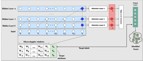
Figure 6 depicts the classification process realized in this study. The figure shows a TCN classifier trained by a set of micro-doppler time windows W. These windows are extracted from the spectrograms, like those shown in Figure 5, and used for neural networks training process. Each set of windows (represented by a row of the table in the lower part of the figure) is computed as a feature vector representing a single instance associated with a multinomial label , which specifies the person identity (target attribute). The spectrograms sliding windows are given as input to the network and are propagated through the layers of the TCN with a dilation factor that doubles on each layer.
In the training step, in order to perform validation, a 10-fold cross-validation is used [32]. Finally, the trained classifier is assessed on a the test set composed of data gathered from walking sessions never used before. The classifier is realized with a TCN architecture [18] that uses a 1D fully-convolutional network (FCN) architecture.
In the proposed architecture, three types of layers are considered: an input layer, a hidden layer, and an attention layer. The input layer is the neural network entry point and includes a node for each set of considered features at a given time.
The hidden layers are instead made of artificial neurons (they are also called “perceptrons”). The output of each neuron is computed as a weighted sum of its inputs and passed through an activation function or a soft-plus function. In the proposed architecture, a different number of hidden layers can be used: all the hidden layers have the same length as the input layer. However, a padding of length (kernel size-1) is added to enforce the layer length coherence and keep subsequent layers at the same length as the previous ones. This architecture allows us to ensure that at each evaluation, the output is obtained by considering only the current and the previous samples. Moreover, the architecture employs dilated convolutions that enable an exponentially large receptive field on the base of a dilation factor (a sort of fixed step) between every two adjacent filters. At the increase of the layer number, the dilation factor grows exponentially. However, when the kernel size is , the data used at the lower layer is and still grows exponentially at the increasing of the network layers. The classification is finally performed on the last sequential activation of the last layer (output layer) which synthesizes the information extracted from the complete input sequence into a single feature vector and produces the requested output.
Moreover, while this representation can be very reductive with respect to the high number of complex relationships, a hierarchical attention mechanism [19] is added across the network layers similarly to [33,34,35]. Attention layers model the relationships regardless of their distance in the input or output sequences.
Looking at Figure 6, for the TCN having n hidden layers, the weights matrix is defined as:
where i is the layer number containing the convolutional activations (with ), K is the filters’ number at each layer and T is the length of the window.
Moreover, we can define the layer attention weight as:
where are the trainable parameter vectors. For the layer i, the corresponding set of convolutional activations is computed as where is one activation function among ReLU, Mish and Swish [36] and are the weights of the attention layer. Finally, the convolutional activations of the hidden layers allow to compute the representation of the last sequence to ensure the final classification:
where and are respectively the vector of weights and the output of the high-level attention layer, and is the neural network final. Notice that, the batch normalization [37] is also added to improve the training of deep feed-forward neural networks. In the training step, we tested different combinations of architectural parameters (i.e., number of layers, batch size, optimization algorithm, and activation functions) to optimize the classifier’s performance. The training is also performed with a cross-entropy loss function [38], optimized thought a stochastic gradient descent (SGD) technique. The adopted momentum is equal to 0.09 while the fixed decay is . The learning performances are also improved by configuring the SGD into all experiments with Nesterov accelerated gradient (NAG) correction (this allows to avoid excessive changes in the parameter space) [39].
4. Validation and Assessment
4.1. Dataset Construction
The dataset selected in this work is the public dataset acquired by the University of Glasgow (http://researchdata.gla.ac.uk/848/) containing C-band (carrier 5.8 GHz) micro-Doppler signatures of different human activities performed by different subjects in different environments [40]. The dataset has been acquired from individuals of male and female sex, left and right handed, aged between 21 and 98 years old and with an height interval between 149–198 cm. Each subject in the dataset performs the following activities 3 times: walking back and forth, sitting down on a chair, standing up, bending to pick up an object, drinking from a cup or glass and in some cases falls were also simulated. In this work only the acquisitions containing the subjects walking back and forth were considered, thus all the other activities were discarded and are not considered in this work. Compared with the dataset used in [20], this dataset is more challenging as presents data acquired with a lower carrier frequency (5.8 GHz vs. 77 GHz used in [20]) from a large number of subjects and in different environments. The total number of different individuas is 106 with a total number of 318 observations available from the various walking sessions. For each activity a spectrogram computed according to Equation (3) is obtained using three different Hamming windows of 0.5, 1 and 2 millisecond window with 98% overlap. The 3 different window sizes will be used in different testing setups to assess the influence of the time-frequency resolution trade-off. The MD signal is finally re-organized into windows with a length of 25.5 s of data with an overlap of 1 s, for the generation of both the validation and test set.
4.2. Experimental Settings
The proposed experiment aims to evaluate the effectiveness of our approach to identify a single walker with respect to the other ones. To this aim, the performances of the proposed classifier are evaluated by computing its precision, recall, F1, Accuracy, and Area Under Curve (AUC) [41] on a real dataset suitable for the feature model described in Section 3. In the assessment step, the best combination of the parameters reported in Table 2 is computed exploiting a Sequential Bayesian Model-based Optimization (SBMO) approach implemented by using a Tree Parzen Estimator (TPE) algorithm [42]. Table 2 lists the considered hyperparameters and their evaluated ranges. As an activation function, the ReLU is evaluated since it is widely adopted. However, it is known that the ReLU activation function suffers from the so-called “dead” units problem. The dying ReLU problem happens if the input becomes too large causing the gradient to update the weights in a way that the summation, and thus the input, will always be less than zero for the remaining of the entire training session. Since ReLU is defined as g(x) = max(0, x), if the input is always less than zero, it could just as well have been g(x) = 0. But since the gradient of a constant function is still zero, the weights won’t be updated anymore leading to the neuron effectively dying being trapped in a bad local minimum. For this reason, in this study also Swish and Mish are activation functions are also evaluated. However, they are recently proposed [36,43] since they are not affected by the “dead neurons” issue and give better performance in the case of the vanishing gradient problem.
For the network size, two levels (small and medium) are evaluated. The small size network has a maximum of 1.5 mln of learning parameters whereas a medium network has a number of parameters greater than 1.5 mln and lower of 7 mln. Looking at the learning rate, we consider a range between 5 and 15. These values are normalized with respect to the used optimization algorithm. For example, when the SGD optimizer is used, the learning rate ranges between 0.09 and 0.12.
The table also reports the evaluated number of layers (from 6 to 9) and the batch size. For the last one, three standard and widely used sizes (64, 128, and 256) are evaluated. Notice that for the batch size we observed that when it is greater than 256 the training process became less stable (this also influence the accuracy result).
Moeover, to minimize the loss, the three evaluated optimization algorithms are: the Stochastic Gradient Descent (SGD) [44], RmsProp [45], Nadam [45]. Finally in the table also the considered window sizes (64, 128 and 256) for the spectrogram computation. These correspond to the 0.5, 1 and 2 milliseconds time windows.
In the proposed experiments, the SGD is integrated with the Nesterov Accelerated Gradient (NAG) correction to reduce the possible changes in the parameter space [39].
The proposed experiments also allow evaluating the impact of the number of identified targets (walkers) on the classifier performance. To this aim, we evaluate the classifier performance when different numbers of subjects (10, 50, 100) are used for the analysis.
The neural network classifier is implemented by using PyTorch 1.4 deep learning framework and the training is performed on a machine with two Intel (R) Core (TM) i9 CPU 4.30 GHZ, 64 GB of RAM, and four Nvidia Titan XP.
4.3. Results and Discussion
Table 3 reports for the classifier performance at the best hyperparameters combinations when the training is performed respectively with a different number of targets (10, 50, 100). Looking at the 100-targets TCN classifier, we notice that the best accuracy (0.89) is reached when the temporal window size (WS) is of 128 seconds. The corresponding hyperparameters configuration provides Mish as activation function (AF), Nadam as optimization algorithms (OA), a large network size (NS), a batch size (BS) of 16, nine hidden layers (NL) and was trained by with learning rate (LR) equal to 0.15.
Figure 7 reports for the best 100-targets TCN classifier, the training and loss accuracy at the increasing of the epochs. The figure highlights that that accuracy and loss became stable starting from 40 epochs.
Table 4 also reports the performance of the TCN for different number of targets compared to the best standard classifiers. Specifically, we compared the proposed architecture with the state of the art models used for similar tasks (i.e., VGG16 and VGG19 [46], RESNET [47], and the standard CNN2D). The table shows that in all the cases the TCN gives best F1 and AUC.
Finally, we also evaluated the impact of the number of targets used for the classifier’s training on its performances.
Starting from Table 3, it is clear that the classifier performances get worse at the increasing of the number of targets used for the training. However, the table also shows that in all the cases the obtained performances are never less than 0.849 (it is the hyperparameters combination describe in the last row of the table). Looking to Table 4, it also clear that in all the tested classifiers the performances are similarly influenced by the number of targets used for the training. These results, for the CNN classifier, are also confirmed by the findings described in [26].
As we can see from Figure 8, F1 decreases when the number of Targets increases but the proposed network (TCN) for a given number of detected users is always the best.
Finally, Figure 9 (left side) show the different F1 scores of the TCN classifiers by the changing targets numbers. Similarly, the figure (right side) also shows that the best F1 score is generally obtained for the window size of 128. The figure confirms and generalizes the above considerations.
From the point of view of the performance of the end-to-end system, it is worth noting that the inference times are very short (in the order of milliseconds for a single image). For this reason the system can be implemented to operate in real time with the largest computational cost residing in the computation of the STFT that is then sent as input to the trained neural network.
5. Conclusions
This study introduces an approach based on a TCN classifier and a set of micro-Doppler features. The approach aims to perform gait recognition using the data extracted by a low-cost low-power FMCW radar. The accuracy of the classifier is evaluated on a real dataset acquired by the University of Glasgow. The dataset contains data gathered from walking sessions involving a total number of 106 different individuals a total number of 318 observations available from the various walking sessions. The performance of the TCN classifier is evaluated considering different hyper-parameters combinations, different window sizes, and different numbers of targets. In all the cases, the results show the greater performance of the TCN classifier with respect to other baseline ones (CNN2D, RESNET, VGG16, and VGG19).
Finally, we also observed that the number of targets used for the classifier’s training and the window size influence the classifier performances. However, the classifier performances get worse with an increase in the number of targets used for the training. Moreover, the best F1 score is obtained when the windows size is 128, probably because that is the best tradeoff between time and frequency resolution. The results confirm that 8-layer TCN networks, augmented with hierarchical attention layers, are suitable for identification of up to a hundred of walkers with good quality classification performances (F1 = 0.9).
Author Contributions
Data curation, M.L.B.; Formal analysis, P.A., M.L.B. and M.C.; Investigation, M.C.; Methodology, M.C.; Software, M.L.B. and M.C.; Supervision, C.C. and D.O.; Validation, M.L.B.; Writing – original draft, M.C. and C.C.; Writing – review & editing, P.A., M.L.B., F.B., M.C., C.C. and D.O. All authors have read and agreed to the published version of the manuscript.
Funding
This research received no funding.
Institutional Review Board Statement
Not applicable.
Informed Consent Statement
Not applicable.
Data Availability Statement
Not applicable.
Conflicts of Interest
The authors declare no conflict of interest.
References
- Saponara, S.; Neri, B. Radar Sensor Signal Acquisition and Multidimensional FFT Processing for Surveillance Applications in Transport Systems. IEEE Trans. Instrum. Meas. 2017, 66, 604–615. [Google Scholar] [CrossRef]
- Kim, B.s.; Jin, Y.; Kim, S.; Lee, J. A Low-Complexity FMCW Surveillance Radar Algorithm Using Two Random Beat Signals. Sensors 2019, 19, 608. [Google Scholar] [CrossRef] [PubMed] [Green Version]
- Björklund, S.; Johansson, T.; Petersson, H. Evaluation of a micro-Doppler classification method on mm-wave data. In Proceedings of the 2012 IEEE Radar Conference, Atlanta, GA, USA, 7–11 May 2012; pp. 934–939. [Google Scholar] [CrossRef]
- Izzo, A.; Ausiello, L.; Clemente, C.; Soraghan, J.J. Loudspeaker Analysis: A Radar Based Approach. IEEE Sens. J. 2020, 20, 1223–1237. [Google Scholar] [CrossRef] [Green Version]
- Chen, V.C.; Li, F.; Ho, S.; Wechsler, H. Micro-Doppler effect in radar: Phenomenon, model, and simulation study. IEEE Trans. Aerosp. Electron. Syst. 2006, 42, 2–21. [Google Scholar] [CrossRef]
- Chen, V. The Micro-Doppler Effect in Radar, 2nd ed.; Artech House: Norwood, MA, USA, 2019. [Google Scholar]
- Clemente, C.; Pallotta, L.; De Maio, A.; Soraghan, J.J.; Farina, A. A novel algorithm for radar classification based on doppler characteristics exploiting orthogonal Pseudo-Zernike polynomials. IEEE Trans. Aerosp. Electron. Syst. 2015, 51, 417–430. [Google Scholar] [CrossRef] [Green Version]
- Du, L.; Li, L.; Wang, B.; Xiao, J. Micro-Doppler Feature Extraction Based on Time-Frequency Spectrogram for Ground Moving Targets Classification With Low-Resolution Radar. IEEE Sens. J. 2016, 16, 3756–3763. [Google Scholar] [CrossRef]
- Bai, X.; Zhou, F. Radar imaging of micromotion targets from corrupted data. IEEE Trans. Aerosp. Electron. Syst. 2016, 52, 2789–2802. [Google Scholar] [CrossRef]
- Addabbo, P.; Clemente, C.; Ullo, S.L. Fourier independent component analysis of radar micro-Doppler features. In Proceedings of the 2017 IEEE International Workshop on Metrology for AeroSpace (MetroAeroSpace), Padua, Italy, 21–23 June 2017; pp. 45–49. [Google Scholar] [CrossRef] [Green Version]
- Persico, A.R.; Clemente, C.; Gaglione, D.; Ilioudis, C.V.; Cao, J.; Pallotta, L.; De Maio, A.; Proudler, I.; Soraghan, J.J. On Model, Algorithms, and Experiment for Micro-Doppler-Based Recognition of Ballistic Targets. IEEE Trans. Aerosp. Electron. Syst. 2017, 53, 1088–1108. [Google Scholar] [CrossRef] [Green Version]
- Narayanan, R.M.; Zenaldin, M. Radar micro-Doppler signatures of various human activities. IET Radar Sonar Navig. 2015, 9, 1205–1215. [Google Scholar] [CrossRef]
- Le, H.T.; Phung, S.L.; Bouzerdoum, A. Human Gait Recognition with Micro-Doppler Radar and Deep Autoencoder. In Proceedings of the 2018 24th International Conference on Pattern Recognition (ICPR), Beijing, China, 20–24 August 2018; pp. 3347–3352. [Google Scholar] [CrossRef]
- Garreau, G.; Andreou, C.M.; Andreou, A.G.; Georgiou, J.; Dura-Bernal, S.; Wennekers, T.; Denham, S. Gait-based person and gender recognition using micro-doppler signatures. In Proceedings of the 2011 IEEE Biomedical Circuits and Systems Conference (BioCAS), San Diego, CA, USA, 10–12 November 2011; pp. 444–447. [Google Scholar] [CrossRef]
- Cao, P.; Xia, W.; Ye, M.; Zhang, J.; Zhou, J. Radar-ID: Human identification based on radar micro-Doppler signatures using deep convolutional neural networks. IET Radar Sonar Navig. 2018, 12, 729–734. [Google Scholar] [CrossRef]
- Vandersmissen, B.; Knudde, N.; Jalalvand, A.; Couckuyt, I.; Bourdoux, A.; De Neve, W.; Dhaene, T. Indoor Person Identification Using a Low-Power FMCW Radar. IEEE Trans. Geosci. Remote Sens. 2018, 56, 3941–3952. [Google Scholar] [CrossRef] [Green Version]
- Deng, L.; Yu, D. Deep learning: Methods and applications. Found. Trends Signal Process. 2014, 7, 197–387. [Google Scholar] [CrossRef] [Green Version]
- Bai, S.; Kolter, J.Z.; Koltun, V. An Empirical Evaluation of Generic Convolutional and Recurrent Networks for Sequence Modeling. arXiv 2018, arXiv:1803.01271. [Google Scholar]
- Yang, Z.; Yang, D.; Dyer, C.; He, X.; Smola, A.; Hovy, E. Hierarchical Attention Networks for Document Classification. In Proceedings of the 2016 Conference of the North American Chapter of the Association for Computational Linguistics: Human Language Technologies, San Diego, CA, USA, 12–17 June 2016; Association for Computational Linguistics: San Diego, CA, USA, 2016; pp. 1480–1489. [Google Scholar] [CrossRef] [Green Version]
- Addabbo, P.; Bernardi, M.L.; Biondi, F.; Cimitile, M.; Clemente, C.; Orlando, D. Gait Recognition using FMCW Radar and Temporal Convolutional Deep Neural Networks. In Proceedings of the 2020 IEEE 7th International Workshop on Metrology for AeroSpace (MetroAeroSpace), Pisa, Italy, 22–24 June 2020; pp. 171–175. [Google Scholar] [CrossRef]
- Tahmoush, D.; Silvious, J. Radar micro-doppler for long range front-view gait recognition. In Proceedings of the 2009 IEEE 3rd International Conference on Biometrics: Theory, Applications, and Systems, Washington, DC, USA, 28–30 September 2009; pp. 1–6. [Google Scholar] [CrossRef]
- Zhang, Z.; Andreou, A.G. Human identification experiments using acoustic micro-Doppler signatures. In Proceedings of the 2008 Argentine School of Micro-Nanoelectronics, Technology and Applications, Buenos Aires, Argentina, 18–19 September 2008; pp. 81–86. [Google Scholar]
- Reynolds, D. Gaussian Mixture Models. In Encyclopedia of Biometrics; Li, S.Z., Jain, A., Eds.; Springer US: Boston, MA, USA, 2009; pp. 659–663. [Google Scholar] [CrossRef]
- Giorgi, G.; Martinelli, F.; Saracino, A.; Alishahi, M.S. Walking Through the Deep: Gait Analysis for User Authentication through Deep Learning. In IFIP Advances in Information and Communication Technology, Proceedings of the SEC: IFIP International Conference on ICT Systems Security and Privacy Protection, Poznan, Poland, 18–20 September 2018; Springer: Cham, Switzerland, 2018. [Google Scholar]
- Luo, F.; Poslad, S.; Bodanese, E. Human Activity Detection and Coarse Localization Outdoors Using Micro-Doppler Signatures. IEEE Sens. J. 2019, 19, 8079–8094. [Google Scholar] [CrossRef]
- Aloysius, N.; Geetha, M. A review on deep convolutional neural networks. In Proceedings of the 2017 International Conference on Communication and Signal Processing (ICCSP), Chennai, India, 6–8 April 2017; pp. 0588–0592. [Google Scholar] [CrossRef]
- Kim, Y.; Moon, T. Human Detection and Activity Classification Based on Micro-Doppler Signatures Using Deep Convolutional Neural Networks. IEEE Geosci. Remote Sens. Lett. 2016, 13, 8–12. [Google Scholar] [CrossRef]
- Shao, Y.; Dai, Y.; Yuan, L.; Chen, W. Deep Learning Methods for Personnel Recognition Based on Micro-Doppler Features. In Proceedings of the 9th International Conference on Signal Processing Systems, Auckland, New Zealand, 27–30 November 2017; Association for Computing Machinery: New York, NY, USA, 2017; pp. 94–98. [Google Scholar] [CrossRef]
- Chen, V.; Ling, H. Time-Frequency Transforms for Radar Imaging and Signal Analysis; Artech: Morristown, NJ, USA, 2001. [Google Scholar]
- Chen, V.C. Analysis of radar micro-Doppler with time-frequency transform. In Proceedings of the Tenth IEEE Workshop on Statistical Signal and Array Processing (Cat. No.00TH8496), Pocono Manor, PA, USA, 16 August 2000; pp. 463–466. [Google Scholar] [CrossRef]
- Boulic, R.; Thalmann, N.; Thalmann, D.A. A global human walking model with real-time kinematic personification. Vis. Comput. 1990, 6, 344–358. [Google Scholar] [CrossRef]
- Stone, M. Cross-validatory choice and assessment of statistical predictions. R. Stat. Soc. 1974, 36, 111–147. [Google Scholar] [CrossRef]
- Bernardi, M.; Cimitile, M.; Martinelli, F.; Mercaldo, F. Driver and path detection through time-series classification. J. Adv. Transp. 2018, 2018. [Google Scholar] [CrossRef]
- Ardimento, P.; Aversano, L.; Bernardi, M.L.; Cimitile, M. Temporal Convolutional Networks for Just-in-Time Software Defect Prediction. In Proceedings of the 15th International Conference on Software Technologies, ICSOFT 2020, Lieusaint, Paris, France, 7–9 July 2020; van Sinderen, M., Fill, H., Maciaszek, L.A., Eds.; ScitePress: Setúbal, Portugal, 2020; pp. 384–393. [Google Scholar] [CrossRef]
- Bernardi, M.L.; Cimitile, M.; Martinelli, F.; Mercaldo, F. Keystroke Analysis for User Identification using Deep Neural Networks. In Proceedings of the 2019 International Joint Conference on Neural Networks (IJCNN), Budapest, Hungary, 14–19 July 2019; pp. 1–8. [Google Scholar] [CrossRef]
- Misra, D. Mish: A Self Regularized Non-Monotonic Neural Activation Function. arXiv 2019, arXiv:1908.08681. [Google Scholar]
- Ioffe, S.; Szegedy, C. Batch Normalization: Accelerating Deep Network Training by Reducing Internal Covariate Shift. In Proceedings of the 32nd International Conference on International Conference on Machine Learning, Lille, France, 7–9 July 2015; Volume 37, pp. 448–456. [Google Scholar]
- Mannor, S.; Peleg, D.; Rubinstein, R. The Cross Entropy Method for Classification. In Proceedings of the 22nd International Conference on Machine Learning, Bonn, Germany, 7–11 August 2005; pp. 561–568. [Google Scholar]
- Sutskever, I.; Martens, J.; Dahl, G.; Hinton, G. On the Importance of Initialization and Momentum in Deep Learning. In Proceedings of the 30th International Conference on International Conference on Machine Learning, Atlanta, GA, USA, 17–19 June 2013; Volume 28, pp. III-1139–III-1147. [Google Scholar]
- Fioranelli, D.F.; Shah, D.S.A.; Li1, H.; Shrestha, A.; Yang, D.S.; Kernec, D.J.L. Radar sensing for healthcare. Electron. Lett. 2019, 55, 1022–1024. [Google Scholar] [CrossRef] [Green Version]
- Powers, D.M.W. Evaluation: From precision, recall and f-measure to roc., informedness, markedness & correlation. J. Mach. Learn. Technol. 2011, 2, 37–63. [Google Scholar]
- Bergstra, J.; Bardenet, R.; Bengio, Y.; Kégl, B. Algorithms for Hyper-Parameter Optimization. In Proceedings of the 24th International Conference on Neural Information Processing Systems, Granada, Spain, 12–14 December 2011; Curran Associates Inc.: Red Hook, NY, USA, 2011; pp. 2546–2554. [Google Scholar]
- Ramachandran, P.; Zoph, B.; Le, Q.V. Searching for Activation Functions. arXiv 2017, arXiv:1710.05941. [Google Scholar]
- Schaul, T.; Antonoglou, I.; Silver, D. Unit Tests for Stochastic Optimization. arXiv 2013, arXiv:1312.6055. [Google Scholar]
- Wang, Y.; Liu, J.; Mišić, J.; Mišić, V.B.; Lv, S.; Chang, X. Assessing Optimizer Impact on DNN Model Sensitivity to Adversarial Examples. IEEE Access 2019, 7, 152766–152776. [Google Scholar] [CrossRef]
- Liu, S.; Deng, W. Very deep convolutional neural network based image classification using small training sample size. In Proceedings of the 2015 3rd IAPR Asian Conference on Pattern Recognition (ACPR), Kuala Lumpur, Malaysia, 3–6 November 2015; pp. 730–734. [Google Scholar] [CrossRef]
- He, K.; Zhang, X.; Ren, S.; Sun, J. Deep Residual Learning for Image Recognition. In Proceedings of the 2016 IEEE Conference on Computer Vision and Pattern Recognition (CVPR), Las Vegas, NV, USA, 26 June–1 July 2016; pp. 770–778. [Google Scholar] [CrossRef] [Green Version]
Figure 1.
Observation geometry.

Figure 2.
Human walking trajectories.

Figure 3.
Micro-Doppler (MD) signature of Human Walk [29].
Figure 3.
Micro-Doppler (MD) signature of Human Walk [29].

Figure 4.
MD Feature extraction.

Figure 5.
Spectrograms of two walkers.

Figure 6.
Temporal convolutional network (TCN) classifier architecture.

Figure 7.
Training and validation accuracy and loss by epochs for the best 100-targets TCN classifier.
Figure 7.
Training and validation accuracy and loss by epochs for the best 100-targets TCN classifier.

Figure 8.
Performance of deep neural network for increasing number of identified targets.

Figure 9.
F1 score of the TCN classifier trained with different number of targets (left) and different windows (right).
Figure 9.
F1 score of the TCN classifier trained with different number of targets (left) and different windows (right).


Table 1.
List of used symbols and their meanings.
| range from center of (x’,y’,z’) to radar in (x,y,z) | |
| range from point-target to radar in (x,y,z) | |
| range from point-target to center of (x’,y’,z’) | |
| vibration frequency | |
| azimuth angle of the center of (x’,y’,z’) | |
| elevation angle of center of (x’,y’,z’) | |
| azimuth angle of P relative to center of (x’,y’,z’) | |
| elevation angle of P relative to center of (x’,y’,z’) |
Table 2.
Hyper-parameters Optimization space.
| Hyperparameters | Acronym | Optimized Ranges and Sets |
|---|---|---|
| Activation function | AF | {ReLU, Swish, Mish} |
| Batch size | BS | { 32, 64, 128, 256 } |
| Learning rate | LR | [0.09, 0.15] |
| Network size | NS | {Small, Medium, Large} |
| Number of layers | L | { 6, 7, 8, 9 } |
| Optimization algorithm | OA | {SGD, Nadam, RMSprop} |
| Window size | WS | {64, 128, 256} |
Table 3.
Hyperparameters optimization summary: best three.
| Targets | AF | NS | LR | NL | BS | OA | WS | Precision | Recall | F1 | Accuracy | AUC |
|---|---|---|---|---|---|---|---|---|---|---|---|---|
| Swish | Medium | 0.12 | 6 | 64 | Nadam | 128 | 0.984 | 0.978 | 0.991 | 0.984 | 0.989 | |
| 10 | ReLu | Medium | 0.15 | 6 | 128 | SGD | 128 | 0.970 | 0.963 | 0.977 | 0.968 | 0.971 |
| ReLu | Small | 0.09 | 8 | 128 | SGD | 64 | 0.952 | 0.952 | 0.960 | 0.950 | 0.961 | |
| Mish | Large | 0.12 | 7 | 32 | Nadam | 128 | 0.852 | 0.901 | 0.922 | 0.911 | 0.916 | |
| 50 | Swish | Medium | 0.10 | 8 | 32 | SGD | 128 | 0.798 | 0.839 | 0.892 | 0.871 | 0.895 |
| Swish | Medium | 0.12 | 8 | 64 | SGD | 128 | 0.773 | 0.811 | 0.872 | 0,825 | 0.859 | |
| Mish | Large | 0.15 | 9 | 16 | Nadam | 128 | 0.849 | 0.898 | 0.885 | 0.891 | 0.890 | |
| 100 | Mish | Large | 0.14 | 9 | 32 | RMSProp | 128 | 0.830 | 0.851 | 0.838 | 0.862 | 0.871 |
| Mish | Large | 0.15 | 9 | 32 | SGD | 256 | 0.789 | 0.823 | 0.788 | 0.838 | 0.849 |
Table 4.
Performance comparison of the TCN classifiers with baseline methods (CNN2D, RESNET, VGG16, VGG19).
Table 4.
Performance comparison of the TCN classifiers with baseline methods (CNN2D, RESNET, VGG16, VGG19).
| Target | Network | Accuracy | Precision | Recall | F1 | AUC |
|---|---|---|---|---|---|---|
| VGG16 | 0,886 | 0.918 | 0.921 | 0.919 | 0.920 | |
| VGG19 | 0.932 | 0.948 | 0.983 | 0.965 | 0.969 | |
| 10 | RESNET | 0.969 | 0.960 | 0.982 | 0.971 | 0.973 |
| CNN2D | 0.879 | 0.856 | 0.926 | 0.890 | 0.890 | |
| TCN | 0.984 | 0.978 | 0.991 | 0.984 | 0.989 | |
| VGG16 | 0.832 | 0.897 | 0.843 | 0.869 | 0.872 | |
| VGG19 | 0.843 | 0.853 | 0.915 | 0.883 | 0.886 | |
| 50 | RESNET | 0.850 | 0.880 | 0.851 | 0.865 | 0.868 |
| CNN2D | 0.766 | 0.807 | 0.822 | 0.815 | 0.817 | |
| TCN | 0.852 | 0.901 | 0.922 | 0.911 | 0.916 | |
| VGG16 | 0.834 | 0.844 | 0.815 | 0.829 | 0.830 | |
| VGG19 | 0.838 | 0.852 | 0.883 | 0.867 | 0.870 | |
| 100 | RESNET | 0.831 | 0.832 | 0.821 | 0.827 | 0.831 |
| CNN2D | 0.812 | 0.784 | 0.847 | 0.814 | 0.816 | |
| TCN | 0.849 | 0.898 | 0.885 | 0.891 | 0.890 |
Publisher’s Note: MDPI stays neutral with regard to jurisdictional claims in published maps and institutional affiliations. |
© 2021 by the authors. Licensee MDPI, Basel, Switzerland. This article is an open access article distributed under the terms and conditions of the Creative Commons Attribution (CC BY) license (http://creativecommons.org/licenses/by/4.0/).
Share and Cite
MDPI and ACS Style
Addabbo, P.; Bernardi, M.L.; Biondi, F.; Cimitile, M.; Clemente, C.; Orlando, D. Temporal Convolutional Neural Networks for Radar Micro-Doppler Based Gait Recognition. Sensors 2021, 21, 381. https://doi.org/10.3390/s21020381
AMA Style
Addabbo P, Bernardi ML, Biondi F, Cimitile M, Clemente C, Orlando D. Temporal Convolutional Neural Networks for Radar Micro-Doppler Based Gait Recognition. Sensors. 2021; 21(2):381. https://doi.org/10.3390/s21020381
Chicago/Turabian StyleAddabbo, Pia, Mario Luca Bernardi, Filippo Biondi, Marta Cimitile, Carmine Clemente, and Danilo Orlando. 2021. "Temporal Convolutional Neural Networks for Radar Micro-Doppler Based Gait Recognition" Sensors 21, no. 2: 381. https://doi.org/10.3390/s21020381
Note that from the first issue of 2016, this journal uses article numbers instead of page numbers. See further details here.