Identification of Tiny Surface Cracks in a Rugged Weld by Signal Gradient Algorithm Using the ACFM Technique
by
 ,
,
Xin’an Yuan
1, 
Wei Li
1,*,
Xiaokang Yin
1,
Guoming Chen
1,
Jianming Zhao
1,
Weiyu Jiang
1 and
Jiuhao Ge
2 1
Center for Offshore Engineering and Safety Technology, China University of Petroleum (East China), Qingdao 266580, China
2
Nondestructive Detection and Monitoring Technology for High Speed Transportation Facilities, Key Laboratory of Ministry of Industry and Information Technology, Nanjing University of Aeronautics and Astronautics, Nanjing 210016, Jiangsu, China
*
Author to whom correspondence should be addressed.
Sensors 2020, 20(2), 380; https://doi.org/10.3390/s20020380
Submission received: 25 December 2019
/
Revised: 6 January 2020
/
Accepted: 8 January 2020
/
Published: 9 January 2020
(This article belongs to the Special Issue Advanced Magnetic Sensors and Their Applications)
Abstract
:It is still a big challenge to identify tiny surface cracks in a rugged weld due to the lift-off variations using the nondestructive testing (NDT) method. In this paper, the signal gradient algorithm is presented to identify the tiny surface crack in the rugged weld using the alternating current field measurement (ACFM) technique. The ACFM simulation model and testing system was set up to obtain the insensitive signal to the lift-off variations. The signal gradient algorithm was presented to process the insensitive signal for the identification of the tiny surface crack in the rugged weld. The results show that the Bz signal is the insensitive signal to lift-off variations caused by the rugged weld. The signal to noise ratio (SNR) of the crack identification signal was greatly improved by the signal gradient algorithm, and a tiny surface crack can be identified effectively in the weld and the heat affected zone (HAZ).
1. Introduction
The welding procedure is widely used in the manufacturing industry. As a critical connecting portion, it easily introduces cracks in the weld and the HAZ due to the discontinuous material, corrosive environment, varying temperatures, and complex stress. Welds should be inspected routinely using a nondestructive testing (NDT) method in in-service time or before use [1,2,3,4].
Magnetic particle testing (MT) and penetrant testing (PT) are effective methods used to detect surface cracks in a weld. However, the surface of the structure should be cleaned thoroughly, including the coating, the attachment, and the greasy dirt [5,6]. Additionally, the testing result depends on the experience of the operator. Ultrasonic testing (UT) is usually used for the detection of internal defects [7]. Eddy current testing (ET) is easily confused by the lift-off variations, making it hard to identify a tiny crack in a rugged weld [8].
The ACFM technique was developed for the detection of cracks in underwater structures. Due to the advantages of non-contact testing, less cleaning, and quantitative detection, the ACFM technique has been widely used on land and underwater [9,10,11]. The principle of ACFM is shown in Figure 1. The excitation coil induces the local uniform current field in the specimen. When a crack is present, the current field is disturbed. The disturbed current field makes the space magnetic field distorted. The magnetic field in the X direction, Bx (parallel to the crack), shows a trough in the center of the crack which contains depth information of the crack. The magnetic field in the Z direction, Bz (perpendicular to the specimen), shows two opposite peaks at the tips of the crack, which reflects the length of the crack. Normally, a so-called butterfly plot (the Bx against the Bz) is presented to decide whether a crack is present or not. In practice, the cracks are identified by the number of the loops in the butterfly plot after detection [12].
However, when the ACFM is used to detect tiny cracks in a weld, the ripples and reinforcements can be regarded as the distance variations between the probe and the specimen [13] which causes the lift-off of the probe variations, as shown in Figure 2. The lift-off variations bring many interference signals, making the signal to noise ratio (SNR) poor [14,15]. The response signals of a probe are harsh, even on a crack. The Bx and Bz are confused by the noise caused by the lift-off variations. As a result, the conventional butterfly plot cannot effectively identify tiny cracks. Of course, the size of the crack cannot be evaluated by the Bx and Bz at this stage. As the first step, how to find a tiny crack in a weld is critical work in the ACFM field.
The probability of detection (POD) using the ACFM technique decreases drastically for tiny cracks whose lengths are less than 10 mm [16]. Smith et al. applied the ACFM technique to inspect the welds in stainless steel nuclear storage tanks [17]. The results showed that most of the tiny cracks (length less than 10 mm, depth less than 1 mm) could not be identified effectively. Mostafavi et al. presented the mathematical method for the theoretical prediction of the magnetic field distribution around a short crack (length 30 mm) [18]. Yuan et al. presented the two-step interpolation algorithm for the measurement of long and short cracks in the pipe string using the uniform alternating current field [19]. Leng et al. proposed the combined metal magnetic memory (MMM) and the ACFM technique for the detection and evaluation of critical weld joints in a jack-up offshore platform [20]. Rowshandel et al. presented the artificial neural network (ANN) for sizing the important subsurface section of the multiple cracks using ACFM [21]. These methods obtained good characteristic signals from the cracks without lift-off variations [22,23]. However, the characteristic signal and butterfly plot are cluttered when ACFM is used to identify tiny surface cracks in the rugged weld.
The aim of this paper is to find out tiny surface cracks in rugged welds. This paper is organized as follows: in Section 2, the insensitive signal to the lift-off variation is pointed out by simulations and experiments; in Section 3, the tiny crack is detected in the rugged weld and the signal gradient algorithm is presented to identify the tiny crack; and in Section 4, the conclusion and further work are given.
2. Insensitive Signal to Lift-off Variations
2.1. Simulation Model
In terms of the theory, the Bx is produced by the decrease of the current density in the depth direction of the crack. Thus, the Bx keeps an individual value (background signal) when a crack is not present. The Bz is produced by the deflection of the induced current field, thus the Bz is zero when a crack is not present. When the lift-off varies, the background signal changes—but the current field is still uniform (the current density value changes, but still no deflection). Thus, the Bx is easily affected by the lift-off variations and the Bz is insensitive to lift-off variations.
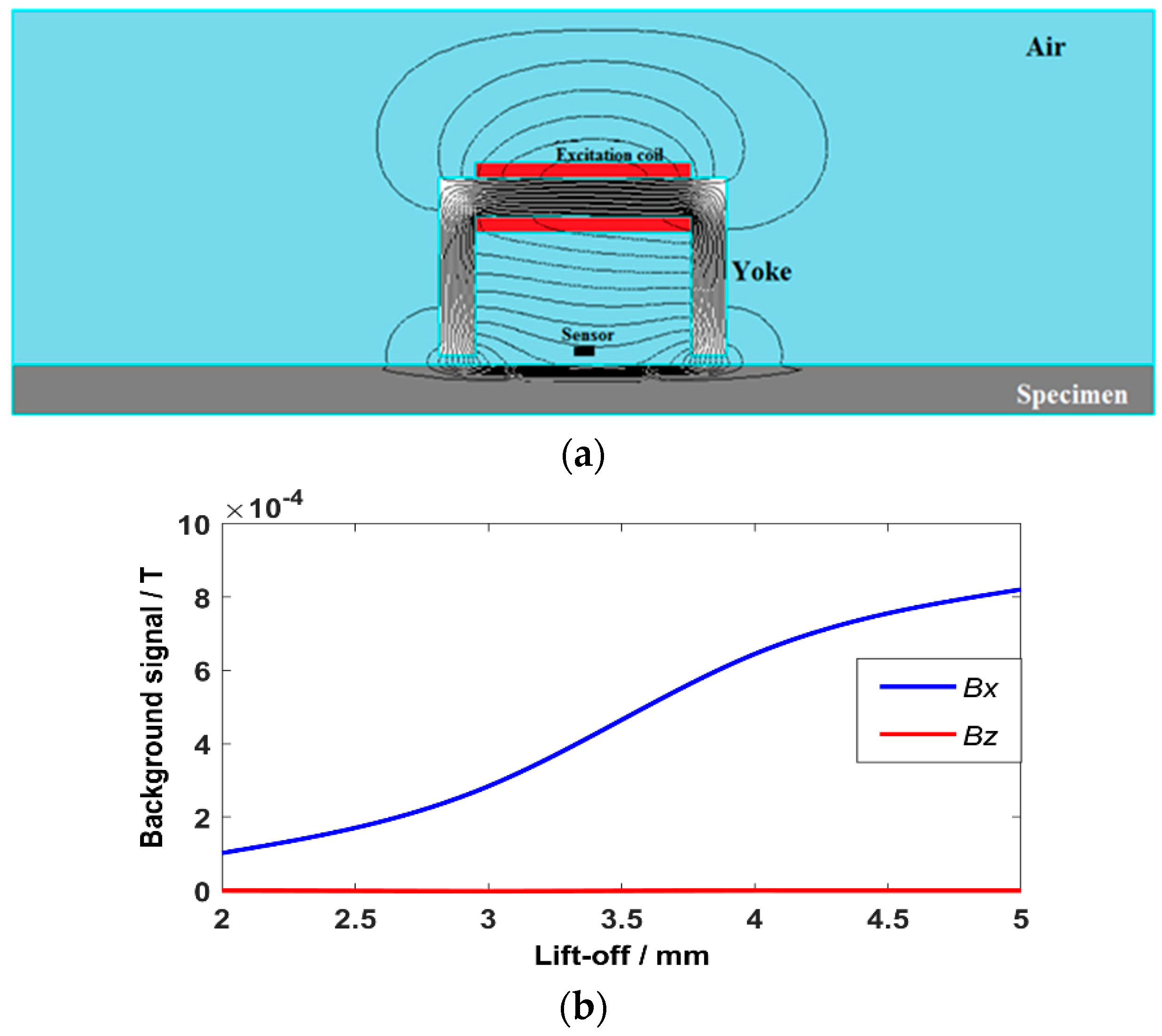
The 2D simulation model of the ACFM probe was set up as shown in Figure 3a. In the model, the frequency is 2 KHz and the current amplitude is 50 mA [24]. The material of the yoke is Mn-Zn ferrite and the specimen is a steel plate. The relative permeability of the yoke is 2000. The conductivity and relative permeability of the specimen are 5 × 10⁶ S/m and 200, respectively. Because steel permeability is much greater than air permeability, the magnetic line of force propagates from the U-shaped yoke to the steel. Meanwhile, due to the skin effect, most of the magnetic line of force gathers in the thin surface of the steel. The magnetic field produces a uniform current field in the center of the specimen [25,26].
When the lift-off increases, more magnetic field leaks into the air. Thus, the background signal of the Bx increases when the lift-off goes up. While there is no magnetic field in the Z direction, the Bz keeps zero because of the uniform current field, as shown in Figure 3b. We can make a conclusion that the Bx is easily affected by the lift-off variations and the Bz is insensitive to the lift-off variations.
2.2. System Set Up
The ACFM testing system is shown in Figure 4a. The system consists of three main parts: a probe, a signal processing box, and a 3-axis scanner. The probe includes an excitation coil, a MnZn-ferrite yoke, a detection sensor, and a primary processing circuit, as shown in Figure 4b. The excitation coil is wound on the MnZn-ferrite yoke with 500 turn enameled wires whose diameter is 0.15 mm. The detection sensor is a 2-axis tunnel magneto resistance (TMR) sensor that is set at the bottom center of the yoke [27,28]. The 2-axis TMR sensor (Type: TMR2303, Capacity: ±80 Oe, Sensitivity: 3 mV/Oe, made by MULTI DIMENSION, China), is used to measure the Bx and Bz at the same time. The Bx and Bz are amplified 50 times and 100 times, respectively, by the primary processing circuit. The thickness of the probe shell bottom is 1 mm to keep the lift-off of the sensor 1 mm. The probe is installed on a 3-axis scanner which is controlled by the programmable logic controller (PLC).
The signal processing box includes a power module, an excitation module, a filtration module, and an acquisition module, as shown in Figure 4b. The power module provides the power source to keep the modules running for more than six hours. The excitation module produces a sinusoidal signal, whose frequency is 2 KHz and amplitude is 10 V. The sinusoidal signal is loaded on the excitation coil in the probe. The Bx and Bz are filtered by the filtration module using a low-pass filter whose cut-off frequency is 20 KHz. The Bx and Bz are gathered by the acquisition module and transmitted to the personal computer (PC) for the signal processing and analyzing software.
2.3. Lift-Off Variation Experiments
To verify the insensitive signal to lift-off variations, the probe is driven up and down above the specimen by the scanner. The first specimen is a mild steel plate with a semi-elliptical artificial crack (length: 50 mm, width: 0.5 mm and depth: 5 mm). There is no weld on the plate and the surface is flat. In the lift-off upward testing experiments, the probe is driven by the scanner to scan along the artificial crack with a lift-off of 1 mm at a speed of 2 mm/s. The probe is raised up 1 mm by the scanner and then dropped after 2 s, as shown in Figure 5a.
As shown in Figure 5b, the Bx shows a trough in the center of the crack, while the Bz shows opposite peaks at the tips of the crack. The characteristic signals are consistent with ACFM theory. When the lift-off is upward, the Bx shows a maximum peak and the Bz remains the same. This is because the background signal increases when the lift-off goes up. Meanwhile, the induced current field is still uniform and the Bz almost remains the same. There are obvious loops in the butterfly plot for the identification of a crack in the flat specimen. The Bx distorted value caused by the 1 mm lift-off variation is much larger than that caused by the crack, which produces an interference signal in the butterfly plot.
In the lift-off downward testing experiments, the probe was lowered down 1 mm by the scanner and then raised after 2 s, as shown in Figure 6a. When the lift-off is downward, the Bx shows a minimum trough and the Bz almost remains the same, as shown in Figure 6b. This is because the background signal decreases when the lift-off goes down. In the same way, the crack can be identified by the butterfly plot. The lift-off downward also produces an obvious interference signal in the butterfly plot.
To simulate the uneven surface of a weld, plastic humps were set on the surface of the specimen in front of the crack, as shown in Figure 7a. When the probe scans the humps, the lift-off varies seriously from 1 mm to 4 mm. The characteristic signals are shown in Figure 7b. The Bx shows hash signals, while the Bz varies slightly in the hump area. The results show that the Bx is affected seriously by the lift-off variations and the Bz is insensitive to the lift-off variations. The Bz can be set as the insensitive signal to identify the tiny surface crack in the weld.
3. Signal Gradient Algorithm
3.1. Detection of Tiny Cracks in the Weld and the HAZ
The second specimen is a plate with one weld, as shown in Figure 8. The material of the specimen is the same as the first specimen. The thickness of the plate is 4 mm. The width of the weld is 10 mm and the height of the weld reinforcement is 2 mm. (The distance between the weld and the HAZ is 2 mm.) The weld ripples are rugged and the thickness of the ripples range from 0.1 mm to 1 mm. Thus, when the ACFM probe scans along the weld, the lift-off of the probe varies from 0.1 mm to 1 mm.
There are three tiny surface cracks in the weld with the same length (4 mm) and different depths (3.5 mm, 3.0 mm and 2.5 mm). There are other 3 cracks with identical length of 4 mm and the same depths (W1, W2, and W3) in the HAZ. The depths of the cracks are given in Table 1.
The probe is driven by the scanner to scan the weld from W1 to H3 at a speed of 5 mm/s. The probe can shake up and down with the ripples. The testing results are shown in Figure 9a. The Bx is chaotic because there are many interference signals caused by the lift-off variations. Thus, the cracks cannot be identified clearly by the Bx signal. There are six characteristic signals in the Bz when a crack is present. The SNR of the Bz is much better than that of the Bx, because the Bz is insensitive to the lift-off variations. As shown in Figure 9b, the butterfly plot is irregular, which cannot be used to identify the 6 tiny cracks.
The third specimen is shown in Figure 10. There are two different length cracks in the HAZ and three different length cracks in the weld. The cracks are at the same depth (3.0 mm). The lengths of the cracks are shown in Table 2.
The weld was scanned at the same speed, and the testing results are shown in Figure 11. The Bx shows two troughs, and the Bz shows two troughs and peaks at the W5 and W6 cracks. The characteristics of the Bx and Bz are incomplete at the W4 crack. For the H4 and H5 cracks, there is one response in the Bx, while the Bz shows slight perturbations because of the very short length of the crack. As shown in Figure 11b, there are two obvious loops in the butterfly plot, which can be used to identify the last two longer cracks in the weld. Other cracks cannot be identified effectively by the irregular tracks in the butterfly plot.
3.2. Signal Gradient Algorithm
The gradient method can find the amplitude change rate of the signal. The Bz changes are small when lift-off varies. Thus, the gradient of the Bz will be zero when a crack is not present. What’s more, there are opposite peaks at the two ends of the crack in the Bz. As a result, a slight perturbation in the Bz caused by the crack is amplified many times by the gradient method. Thus, the gradient of the Bz will show an outstanding peak in the center of the crack. The SNR of the crack identification signal will be improved greatly in the near zero background signal.
The signal gradient algorithm is presented to process the Bz by the following steps, as shown in Figure 12. First, the gradient of the Bz is calculated in real time. If a crack is not present, the value is near zero. When a crack is present, the gradient of the Bz will show some negative values and a major positive value. Then the negative values are decreased and the positive value is magnified. To make the curve smooth, the signal is processed by a 6-th order Butterworth low-pass filter. Thus, the identification signal is presented with a great positive peak and near zero value. The threshold is set beforehand to compare the identification signal with the threshold automatically. If the identification signal is greater than the threshold, the crack can be identified effectively because of the high SNR.
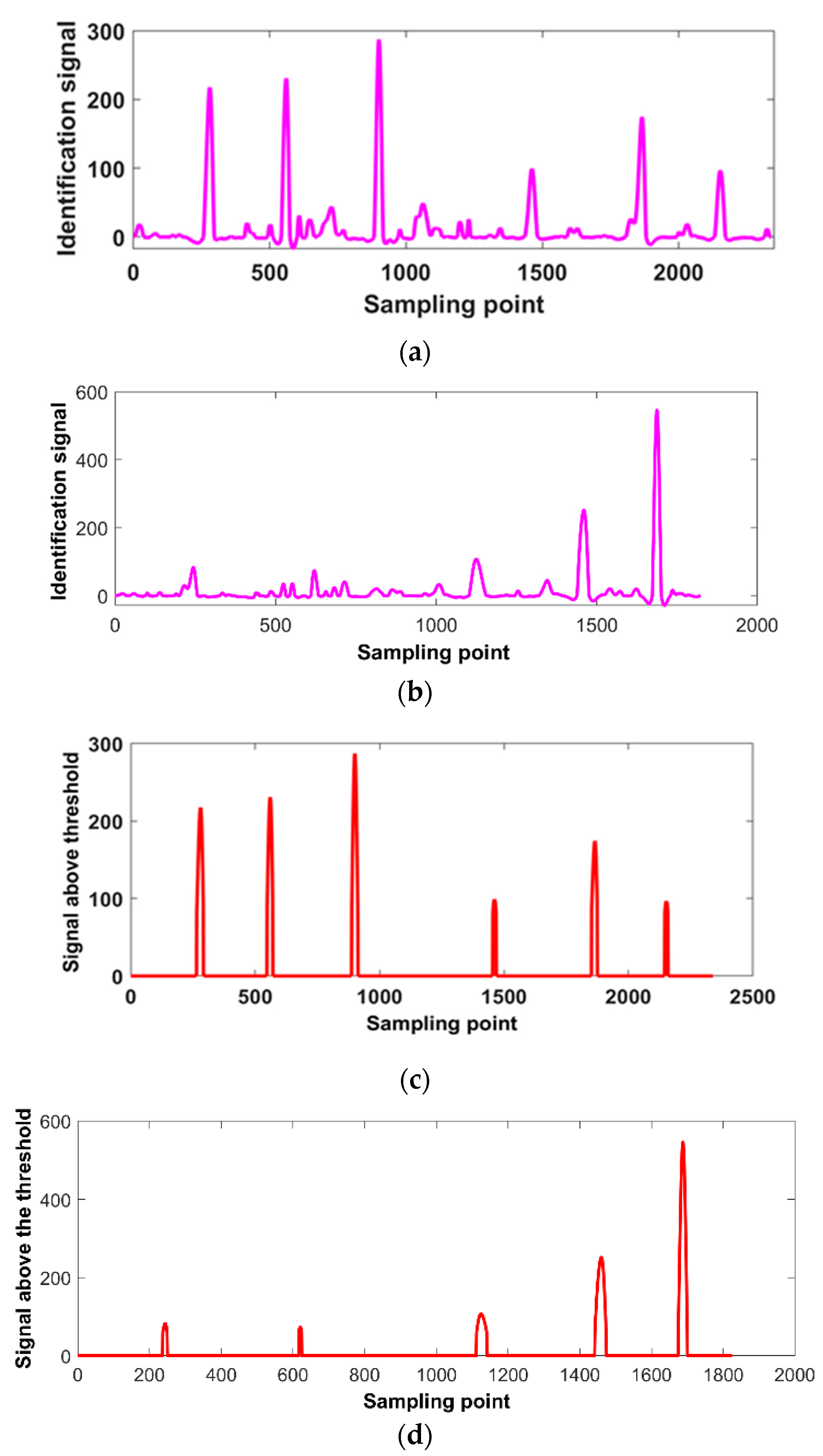
The Bz signals of different depth cracks (from Figure 9a) and different length cracks (from Figure 11a) are processed by the signal gradient algorithm. The identification signals of the tiny surface cracks with lift-off variations in the weld and the HAZ are shown in Figure 13. As shown in Figure 13a, there are six obvious peaks in the identification signals caused by the different length cracks. Meanwhile, there are three obvious peaks caused by the three longer cracks in the weld and two slight peaks caused by the two shorter cracks in the HAZ, as shown in Figure 13b. To remove the background signal and identify the tiny cracks effectively in real time, the threshold can be set in advance using 1.5 times the maximum noise amplitude in the identification signal. In these experiments, the maximum noise amplitude was 53 and the threshold was set as 80. Thus, all six different depth cracks and five different length cracks can be identified effectively, as shown in Figure 13c,d, respectively.
3.3. Discussions
The SNR of the Bz signal is better than that of the Bx in the crack testing results, as shown in Figure 9a. This is because the Bx signals are greatly disturbed by the lift-off variations caused by the rugged weld ripples and reinforcements. The Bz is relatively stable because it is insensitive to the lift-off variations—thus, the Bz is used as the characteristic signal to identify the tiny crack with lift-off variations. As shown in Figure 11a, where the length of the crack is shorter than 4 mm, the distortion of the Bx and Bz decays seriously. This is because the disturbance of the induced current field declines sharply around the short cracks. For the 1 mm and 2 mm length cracks, the induced current field turns slightly and the magnetic field distorts weakly.
As shown in Figure 13a, the last three peaks are less than the first three peaks. This is because the last three cracks are in the HAZ and the distance between the probe and the HAZ is greater than the distance between the probe and the weld. Because the first three cracks are in the rugged weld, the background signal in the identification signal has a bit more clutter than that of the last three cracks. As shown in Figure 13b, the peaks of the three longer cracks are obvious and the peaks of first two shorter cracks are weaker. Because the length of the tiny cracks has a significant impact on the Bx and Bz signals, it is difficult to identify the shorter cracks (less than 2 mm) in the weld and the HAZ—the shorter cracks are easily covered by the noise signal. Overall, in these experiments the SNR of the identification signals must be relatively high to identify all the tiny cracks in the weld and the HAZ by threshold compared to the conventional butterfly plot.
4. Conclusions
In this paper, a signal gradient algorithm was presented to identify tiny cracks in welds using the ACFM technique. The insensitive signal to the lift-off variations was pointed out by the simulations and experiments. The ACFM probe with a 2-axis TMR sensor and testing system were developed. The different depth and different length tiny surface cracks were detected in the rugged weld and the HAZ using an ACFM testing system. The results show that the Bz signal was the insensitive signal to the lift-off variations. The SNR of the crack response signal was greatly improved by the signal gradient algorithm. Thus, all the tiny surface cracks can be effectively identified in the weld and the HAZ by the signal gradient algorithm using the ACFM technique. Further work will focus on the identification of other type defects, evaluation of tiny defects in the weld, and the HAZ.
Author Contributions
Conceived, designed and conducted the experiments, X.Y. (Xin’an Yuan) and W.L.; Formal analysis, X.Y. (Xiaokang Yin); reviewed the paper, X.Y. (Xin’an Yuan) and G.C.; developed the software, J.Z. and J.G.; performed the simulation model, W.J.; wrote the paper, X.Y. (Xin’an Yuan). All authors have read and agreed to the published version of the manuscript.
Funding
This work was funded by the National Key Research and Development Program of China (No. 2017YFC0804503), the National Natural Science Foundation of China (No. 51574276 and No. 51675536), the National Postdoctoral Program for Innovative Talents (No. BX20190386), China Postdoctoral Science Foundation funded project (2019M662461), the Major National Science and Technology Program (No. 2016ZX05028-001-05), the Fundamental Research Funds for the Central Universities (18CX05017A) and Shandong Province Key Research and Development Plan (No. 2018GHY115026).
Acknowledgments
The authors would like to thank the Center for Offshore Engineering and Safety Technology for the specimen.
Conflicts of Interest
The authors declare no conflict of interest.
References
- Taheri, H.; Kilpatrick, M.; Norvalls, M.; Harper, W.J.; Koester, L.W.; Bigelow, T.A.; Bond, L.J. Investigation of nondestructive testing methods for friction stir welding. Metals 2019, 9, 624. [Google Scholar] [CrossRef] [Green Version]
- Wang, R.; Liu, Z.H.; Wu, J.F.; Jiang, B.Y.; Li, B. Research on phased array ultrasonic testing on CFETR vacuum vessel welding. Fusion Eng. Des. 2019, 139, 124–127. [Google Scholar] [CrossRef]
- Gao, X.D.; Du, L.L.; Ma, N.; Zhou, X.H.; Wang, C.Y.; Gao, P.P. Magneto-optical imaging characteristics of weld defects under alternating and rotating magnetic field excitation. Opt. Laser Technol. 2019, 112, 188–197. [Google Scholar] [CrossRef]
- Andreaus, U.; Baragatti, P.; Casini, P.; Iacoviello, D. Experimental damage evaluation of open and fatigue cracks of multi-cracked beams by using wavelet transform of static response via image analysis. Struct. Control Health Monit. 2016, 105, 227–244. [Google Scholar] [CrossRef]
- Shelikhov, G.S.; Glazkov, Y.A. On the improvement of examination questions during the nondestructive testing of magnetic powder. Russ. J. Nondestr. Test. 2011, 47, 112–117. [Google Scholar] [CrossRef]
- Pashagin, A.I.; Shcherbinin, V.E. Indication of magnetic fields with the use of galvanic currents in magnetic-powder nondestructive testing. Russ. J. Nondestr. Test. 2012, 48, 528–531. [Google Scholar] [CrossRef]
- Takiy, A.E.; Kitano, C.; Higuti, R.T.; Granja, S.C.G.; Prado, V.T.; Elvira, L.; Martinez-Graullera, Ó. Ultrasound imaging of immersed plates using high-order Lamb modes at their low attenuation frequency bands. Mech. Syst. Sign. Process. 2017, 96, 321–332. [Google Scholar] [CrossRef] [Green Version]
- Ricci, M.; Silipigni, G.; Ferrigno, L.; Laracca, M.; Adewale, I.; Tian, G.Y. Evaluation of the lift-off robustness of eddy current imaging techniques. NDT E Int. 2017, 85, 43–52. [Google Scholar] [CrossRef]
- Katoozian, D.; Hasanzadeh, R.P.R. A fuzzy error characterization approach for crack depth profile estimation in metallic structures through ACFM data. IEEE T. Magn. 2017, 53, 6202100. [Google Scholar] [CrossRef]
- Lewis, A.M.; Michael, D.H.; Lugg, M.C.; Collins, R. Thin-skin electromagnetic fields around surface-breaking cracks in metals. J. Appl. Phys. 1988, 64, 3777–3784. [Google Scholar] [CrossRef] [Green Version]
- Raine, A. Cost benefit applications using the ACFM technique. Insight 2002, 44, 180–181. [Google Scholar]
- Akbari-Khezri, A.; Sadeghi, S.H.H.; Moini, R.; Sharifi, M. An efficient modeling technique for analysis of AC field measurement probe output signals to improve crack detection and sizing in cylindrical metallic structures. J. Nondestr. Eval. 2016, 35, 9. [Google Scholar] [CrossRef]
- Deng, Z.Y.; Sun, Y.H.; Yang, Y.; Kang, Y.H. Effects of surface roughness on magnetic flux leakage testing of micro-cracks. Meas. Sci. Technol. 2017, 28, 045003. [Google Scholar] [CrossRef]
- Lu, M.Y.; Xu, H.Y.; Zhu, W.Q.; Yin, L.Y.; Qian, Z.; Peyton, A.J.; Yin, W.L. Conductivity lift-off invariance and measurement of permeability for ferrite metallic plates. NDT E Int. 2018, 95, 36–44. [Google Scholar] [CrossRef]
- Andreaus, U.; Casini, P.; Vestroni, F. Nonlinear features in the dynamic response of a cracked beam under harmonic forcing. In Proceeding of the ASME 2005 International Design Engineering Technical Conferences & Computers and Information in Engineering Conference (DETC’05), Long Beach, CA, USA, 24–28 September 2005; pp. 2083–2089. [Google Scholar]
- Shen, J.L.; Zhou, L.; Rowshandel, H.; Nicholson, G.L.; Davis, C.L. Determining the propagation angle for non-vertical surface-breaking cracks and its effect on crack sizing using an ACFM sensor. Meas. Sci. Technol. 2015, 26, 115604. [Google Scholar] [CrossRef]
- Smith, M.; Laenen, C. Inspection of nuclear storage tanks using remotely deployed ACFMT. Insight 2007, 49, 17–20. [Google Scholar] [CrossRef]
- Mostafavi, R.F.; Mirshekar-Syahkal, D. AC fields around short cracks in metals induced by rectangular coils. IEEE Trans. Magn. 1999, 35, 2001–2006. [Google Scholar] [CrossRef]
- Yuan, X.A.; Li, W.; Chen, G.M.; Yin, X.K.; Yang, W.C.; Ge, J.H. Two-step interpolation algorithm for measurement of longitudinal cracks on pipe strings using circumferential current field testing system. IEEE Trans. Ind. Inform. 2018, 14, 394–402. [Google Scholar] [CrossRef]
- Leng, J.C.; Tian, H.X.; Zhou, G.Q.; Wu, Z.M. Joint detection of MMM and ACFM on critical parts of jack-up offshore platform. Ocean Eng. 2017, 35, 34–38. (In Chinese) [Google Scholar]
- Rowshandel, H.; Nicholson, G.L.; Shen, J.L.; Davis, C.L. Characterization of clustered cracks using an ACFM sensor and application of an artificial neural network. NDT E Int. 2018, 98, 80–88. [Google Scholar] [CrossRef]
- Yuan, X.A.; Li, W.; Chen, G.M.; Yin, X.K.; Jiang, W.Y.; Zhao, J.M.; Ge, J.H. Inspection of both inner and outer cracks in aluminum tubes using double frequency circumferential current field testing method. Mech. Syst. Sign. Process. 2019, 127, 16–34. [Google Scholar] [CrossRef]
- Tian, G.Y.; Sophian, A. Reduction of lift-off effects for pulsed eddy current. NDT E Int. 2005, 38, 319–324. [Google Scholar] [CrossRef]
- Yuan, X.A.; Li, W.; Chen, G.M.; Yin, X.K.; Ge, J.H. Frequency optimisation of circumferential current field testing system for highly-sensitive detection of Iongitudinal cracks on a pipe string. Insight 2017, 59, 378–382. [Google Scholar] [CrossRef]
- Li, Y.; Yan, B.; Li, D.; Li, Y.L.; Zhou, D.Q. Gradient-field pulsed eddy current probes for imaging of hidden corrosion in conductive structures. Sens. Actuators A Phys. 2016, 38, 251–265. [Google Scholar] [CrossRef]
- Li, Y.; Ren, S.T.; Yan, B.; Abidin, I.M.Z.; Wang, Y. Imaging of subsurface corrosion using gradient-field pulsed eddy current probes with uniform field excitation. Sensors 2017, 17, 1747. [Google Scholar] [CrossRef]
- Atzlesberger, J.; Zagar, B.G.; Cihal, R.; Brummayer, M.; Reisinger, P. Sub-surface defect detection in a steel sheet. Meas. Sci. Technol. 2013, 24, 084003. [Google Scholar] [CrossRef]
- AbdAlla, A.N.; Faraj, M.A.; Samsuri, F.; Rifai, D.; Ali, K.; Al-Douri, Y. Challenges in improving the performance of eddy current testing: Review. Meas. Control 2019, 52, 46–64. [Google Scholar] [CrossRef] [Green Version]
Figure 1.
Principle of ACFM.
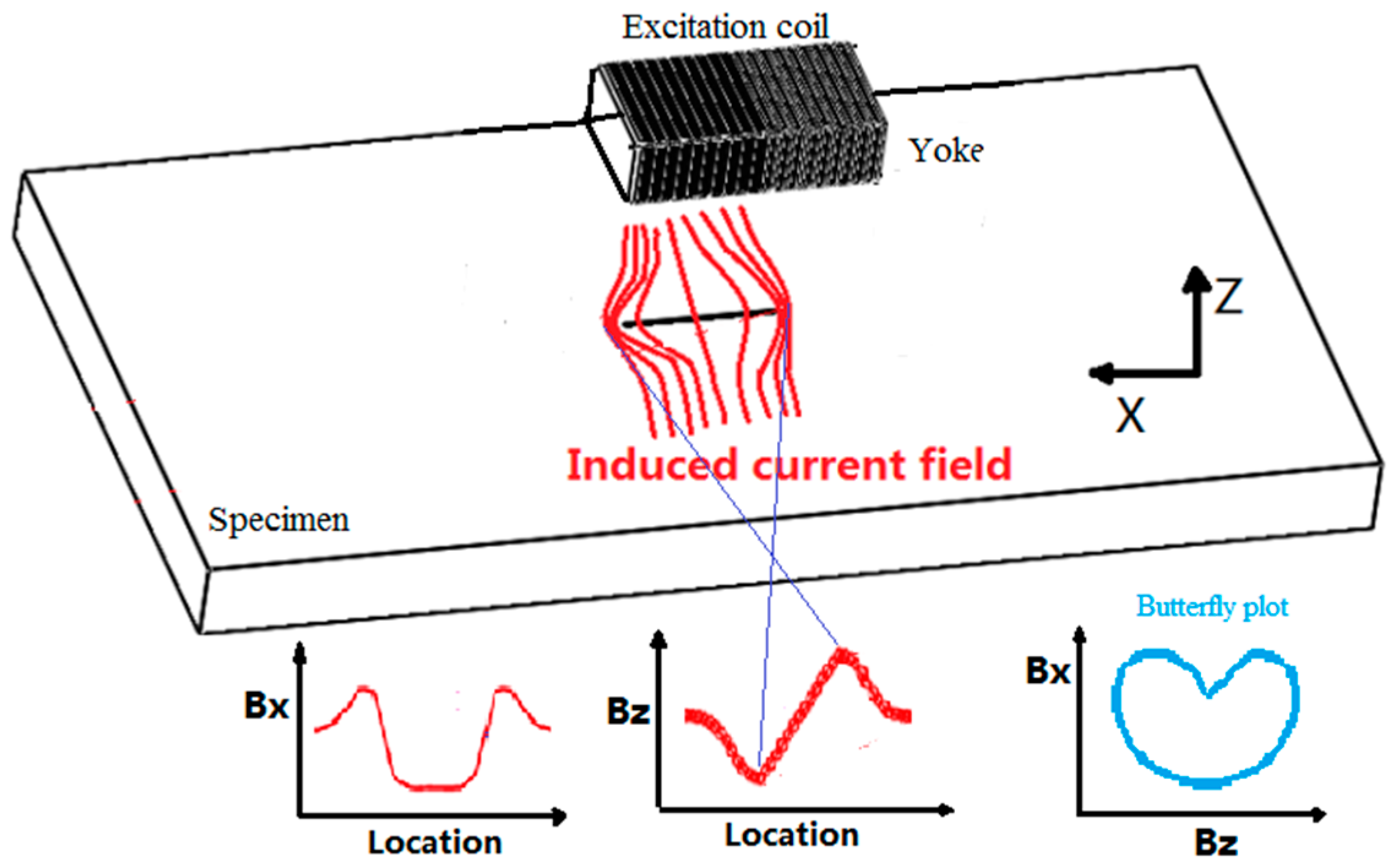
Figure 2.
Weld ripples and reinforcement cause lift-off variations.

Figure 3.
A 2D simulation model of ACFM probe. (a) Distribution of magnetic field; (b) background signal with different lift-off.
Figure 3.
A 2D simulation model of ACFM probe. (a) Distribution of magnetic field; (b) background signal with different lift-off.

Figure 4.
ACFM system. (a) Photo of the system; (b) probe and signal processing module.
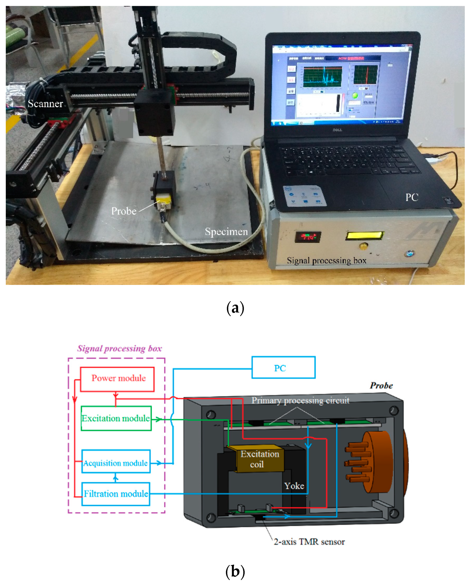
Figure 5.
Testing results when lift-off upward. (a) Probe scan path; (b) Bx, Bz, and butterfly plot.
Figure 5.
Testing results when lift-off upward. (a) Probe scan path; (b) Bx, Bz, and butterfly plot.

Figure 6.
Testing results when probe downward. (a) Probe scan path; (b) Bx, Bz, and butterfly plot.
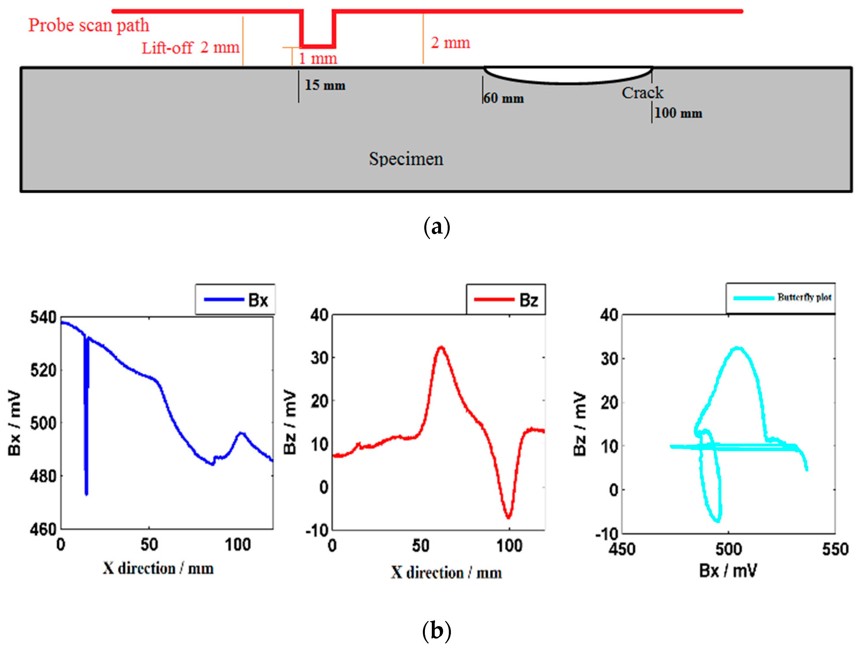
Figure 7.
Testing results when lift-off varies seriously. (a) Probe scan path; (b) Bx, Bz, and butterfly plot.
Figure 7.
Testing results when lift-off varies seriously. (a) Probe scan path; (b) Bx, Bz, and butterfly plot.

Figure 8.
The second specimen with different depth cracks.
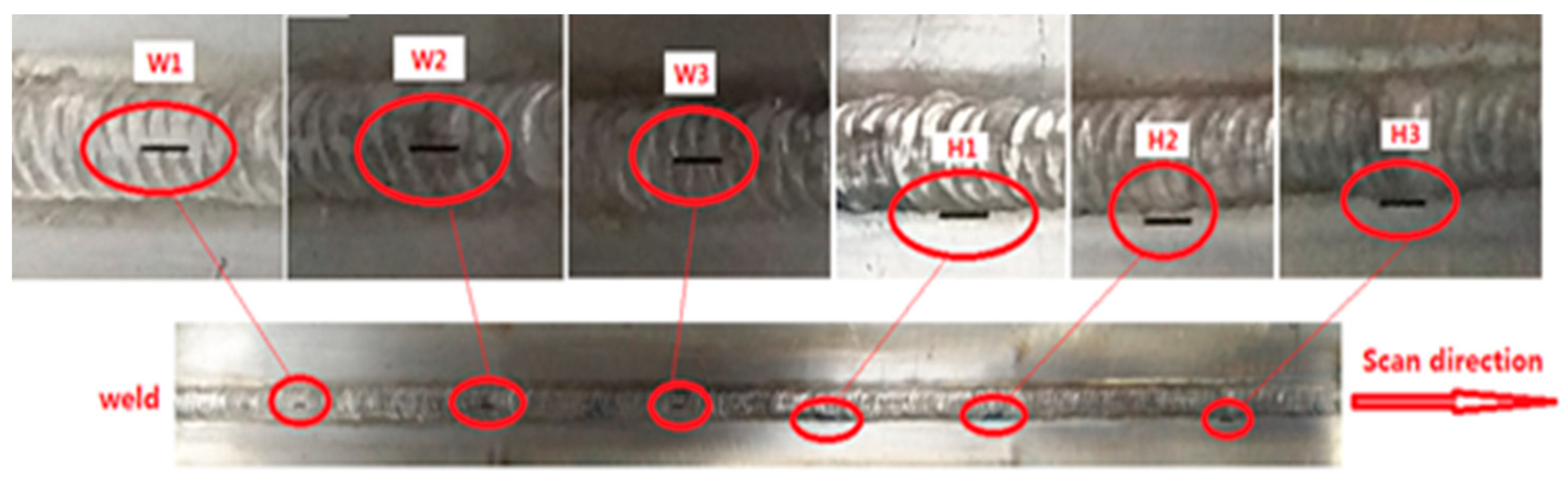
Figure 9.
Characteristic signals of different depth cracks in the weld and the HAZ. (a) Bx and Bz; (b) butterfly plot.
Figure 9.
Characteristic signals of different depth cracks in the weld and the HAZ. (a) Bx and Bz; (b) butterfly plot.


Figure 10.
The third specimen with different length cracks.

Figure 11.
Characteristic signals of different length cracks in the weld and the HAZ. (a) Bx and Bz; (b) butterfly plot.
Figure 11.
Characteristic signals of different length cracks in the weld and the HAZ. (a) Bx and Bz; (b) butterfly plot.
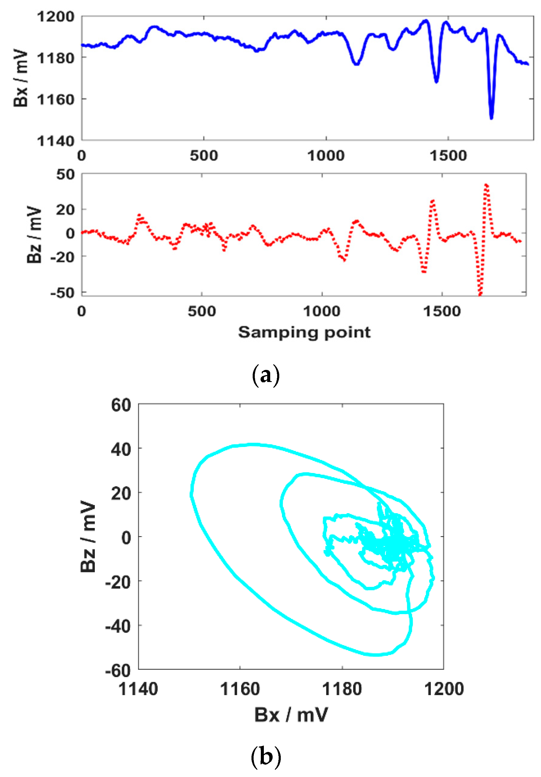
Figure 12.
Signal gradient algorithm for the processes of the Bz.

Figure 13.
Identification of tiny cracks by signal gradient algorithm. (a) Identification signal of different depth cracks; (b) identification signal of different length cracks; (c) identification of different depth tiny cracks; (d) identification of different length tiny cracks.
Figure 13.
Identification of tiny cracks by signal gradient algorithm. (a) Identification signal of different depth cracks; (b) identification signal of different length cracks; (c) identification of different depth tiny cracks; (d) identification of different length tiny cracks.


Table 1.
The depth of the cracks.
| No. | W1 | W2 | W3 | H1 | H2 | H3 |
|---|---|---|---|---|---|---|
| Depth/mm | 3.5 | 3.0 | 2.5 | 3.5 | 3.0 | 2.5 |
Table 2.
The length of the cracks.
| No. | H4 | H5 | W4 | W5 | W6 |
|---|---|---|---|---|---|
| Length/mm | 1.0 | 2.0 | 4.0 | 6.0 | 8.0 |
© 2020 by the authors. Licensee MDPI, Basel, Switzerland. This article is an open access article distributed under the terms and conditions of the Creative Commons Attribution (CC BY) license (http://creativecommons.org/licenses/by/4.0/).
Share and Cite
MDPI and ACS Style
Yuan, X.; Li, W.; Yin, X.; Chen, G.; Zhao, J.; Jiang, W.; Ge, J. Identification of Tiny Surface Cracks in a Rugged Weld by Signal Gradient Algorithm Using the ACFM Technique. Sensors 2020, 20, 380. https://doi.org/10.3390/s20020380
AMA Style
Yuan X, Li W, Yin X, Chen G, Zhao J, Jiang W, Ge J. Identification of Tiny Surface Cracks in a Rugged Weld by Signal Gradient Algorithm Using the ACFM Technique. Sensors. 2020; 20(2):380. https://doi.org/10.3390/s20020380
Chicago/Turabian StyleYuan, Xin’an, Wei Li, Xiaokang Yin, Guoming Chen, Jianming Zhao, Weiyu Jiang, and Jiuhao Ge. 2020. "Identification of Tiny Surface Cracks in a Rugged Weld by Signal Gradient Algorithm Using the ACFM Technique" Sensors 20, no. 2: 380. https://doi.org/10.3390/s20020380
Note that from the first issue of 2016, this journal uses article numbers instead of page numbers. See further details here.