Knowledge-Aided Doppler Beam Sharpening Super-Resolution Imaging by Exploiting the Spatial Continuity Information

 ,
,
Abstract
:1. Introduction
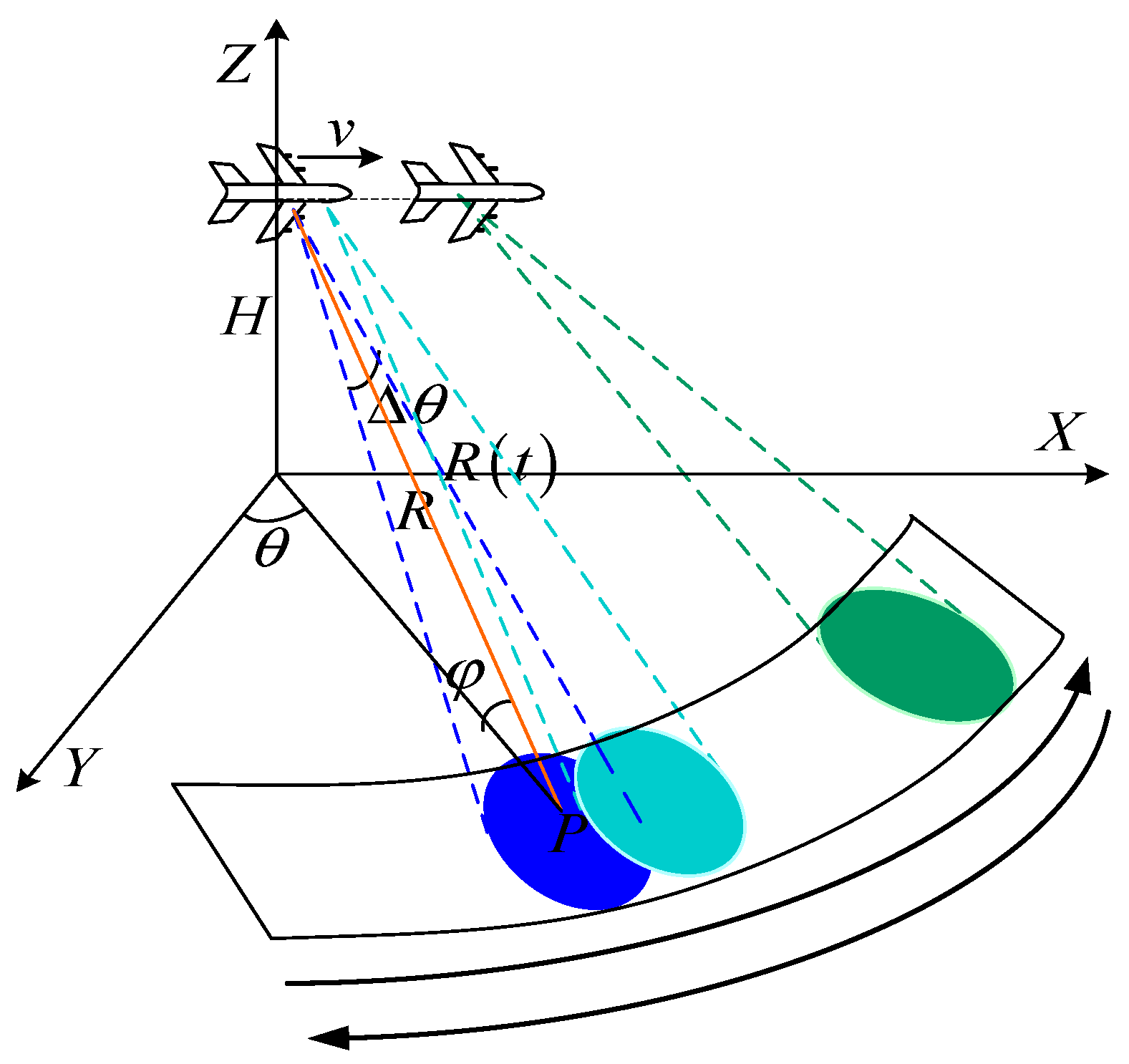
2. DBS Imaging Model
3. Knowledge-Aided DBS Super-Resolution Imaging Algorithm
3.1. Spatial Continuity Property of the Echoed Signal
3.2. KA-DBS Imaging Algorithm
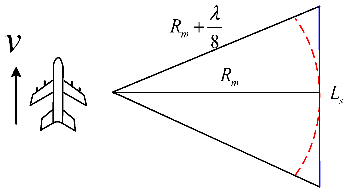
3.3. Performance of the Cross-Range Resolution in KA-DBS
3.4. Super-Resolution Imaging Algorithm Based on KA-DBS
4. Experimental Results
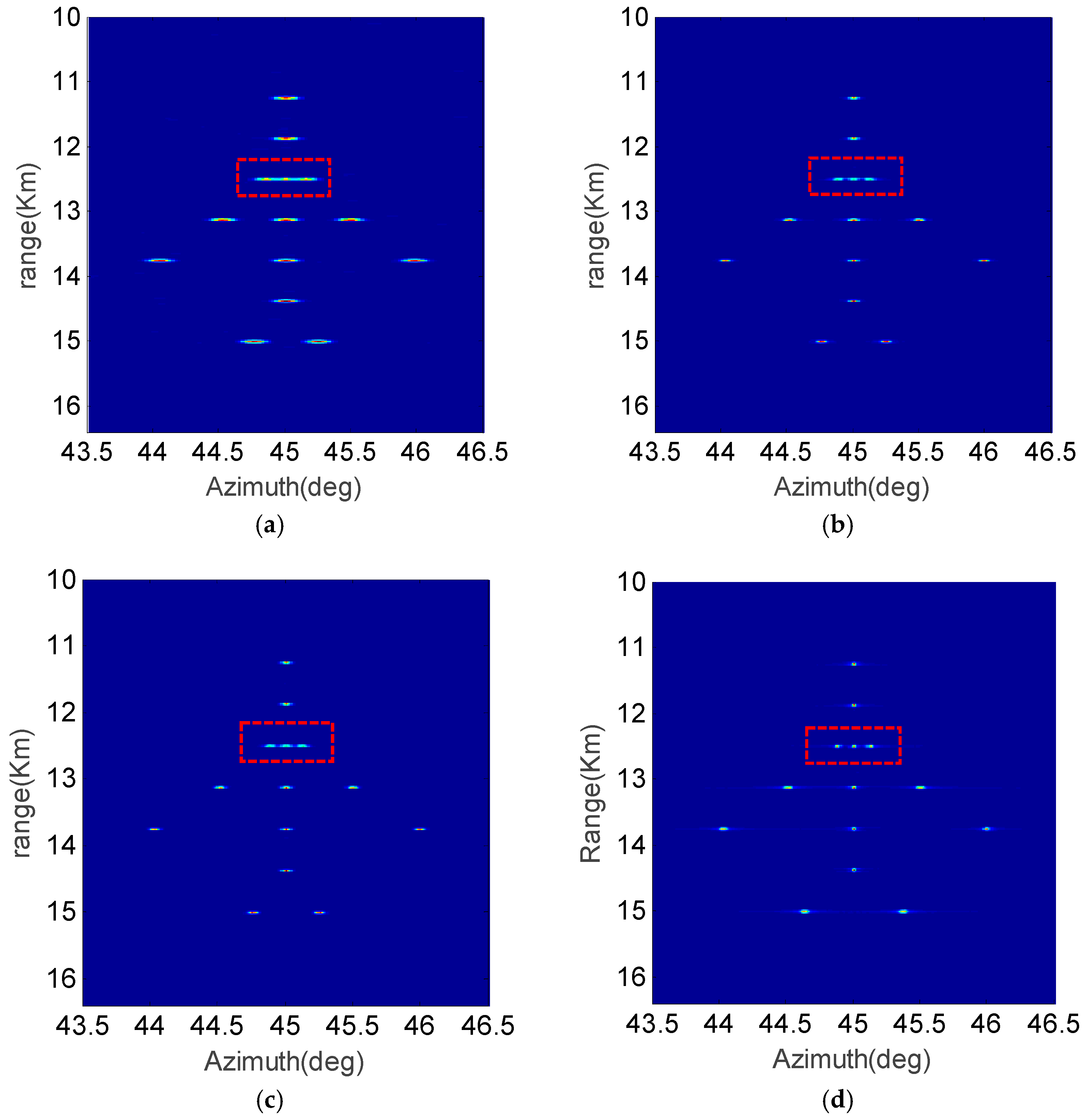
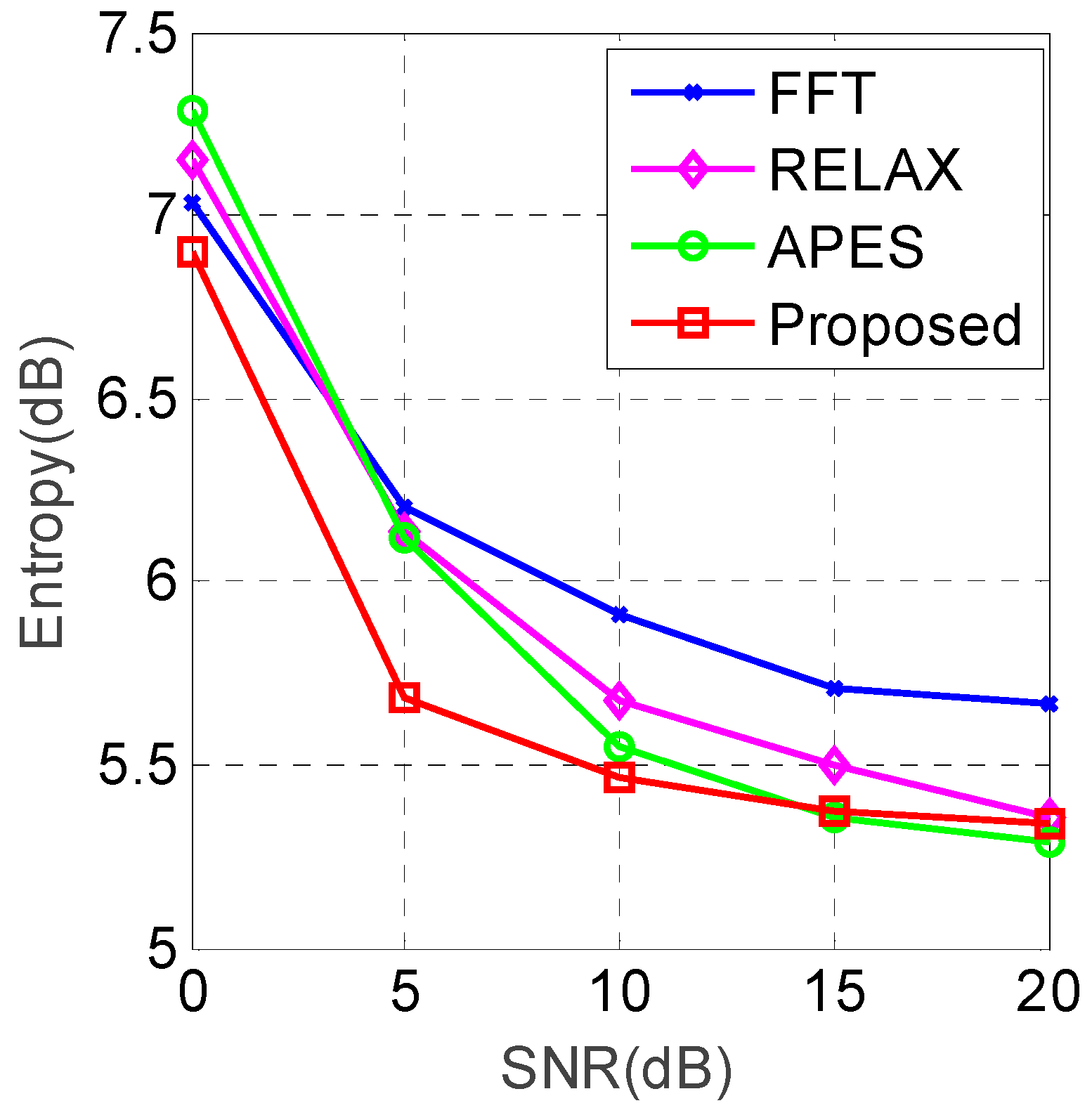
4.1. Simulation
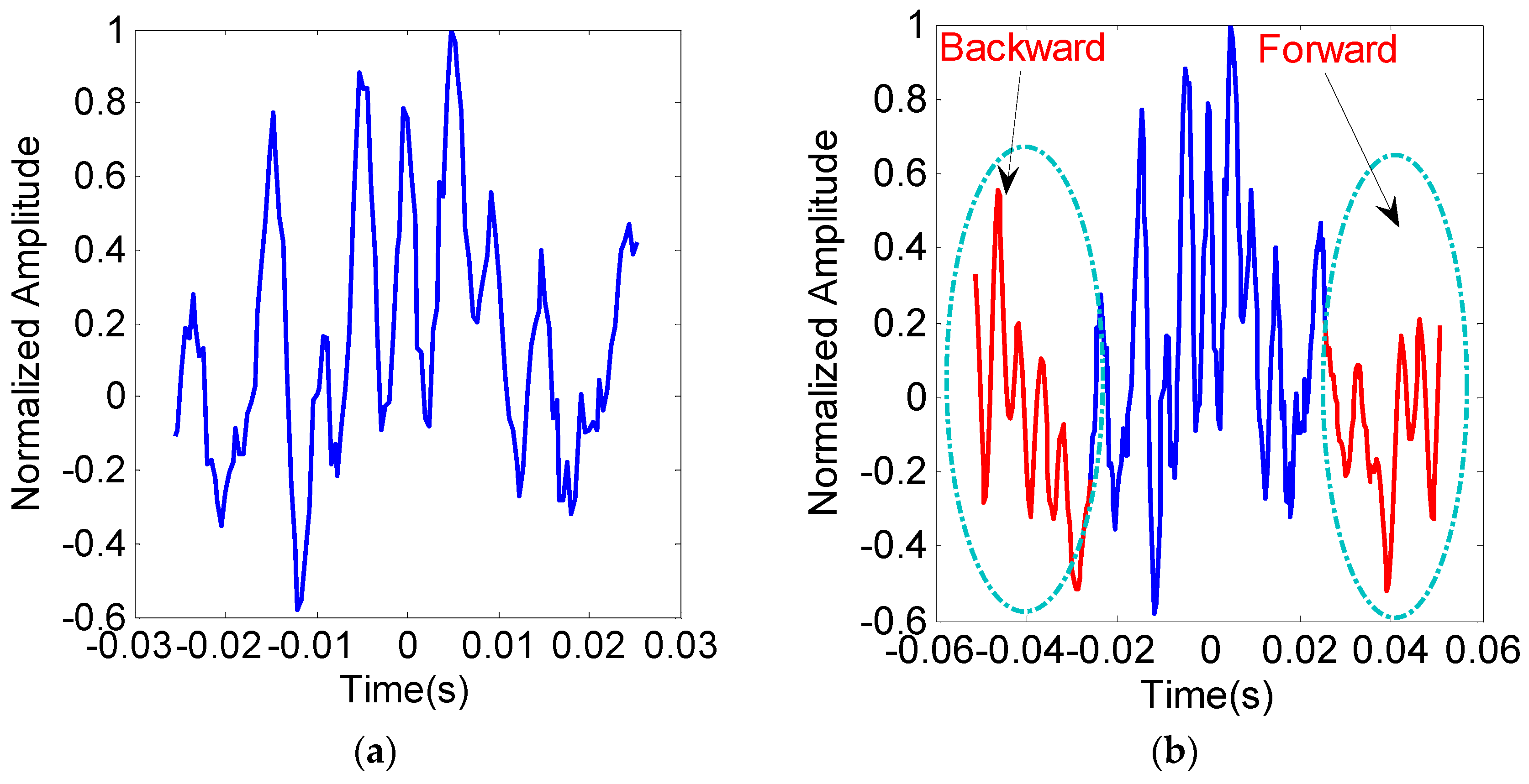
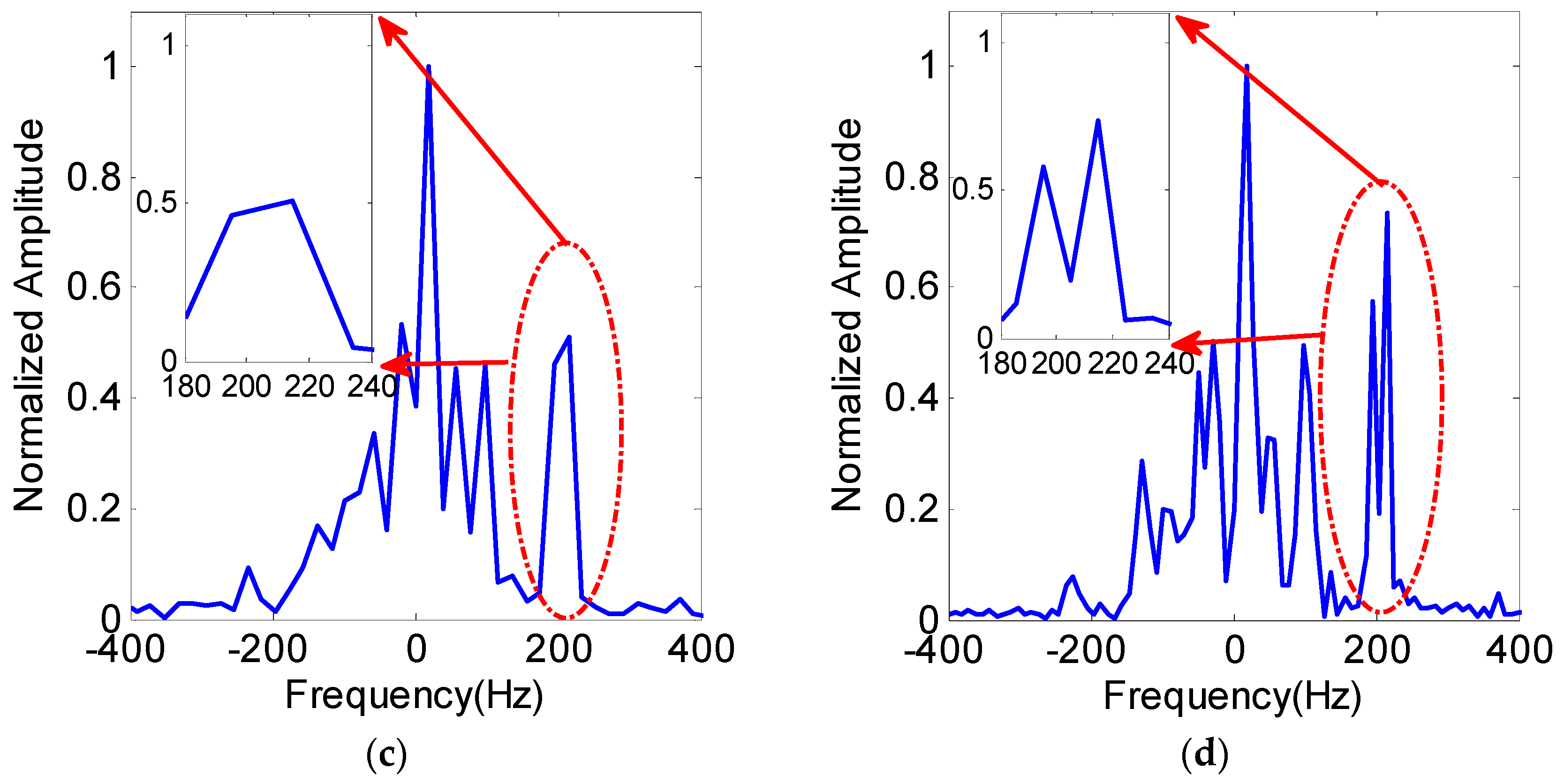
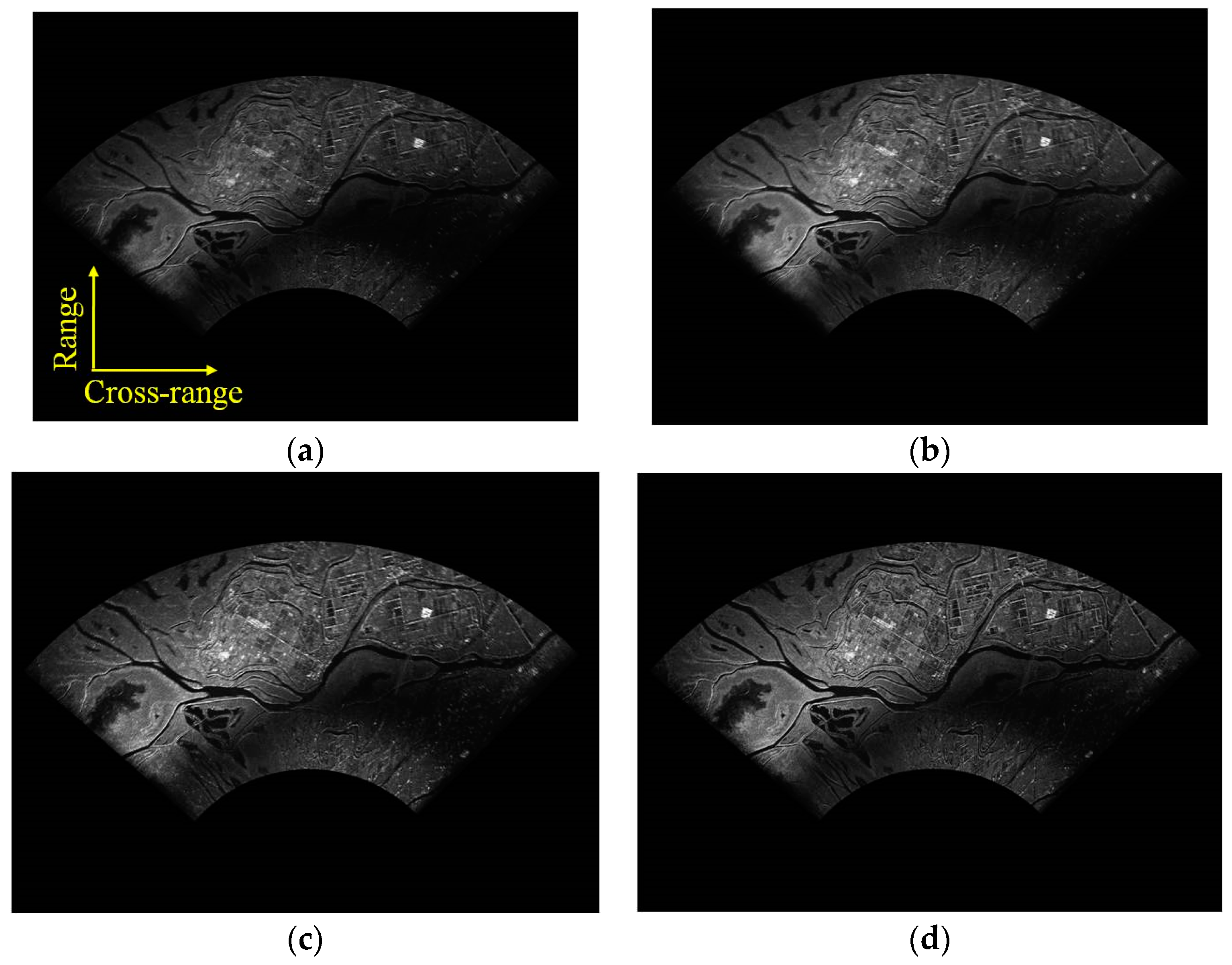
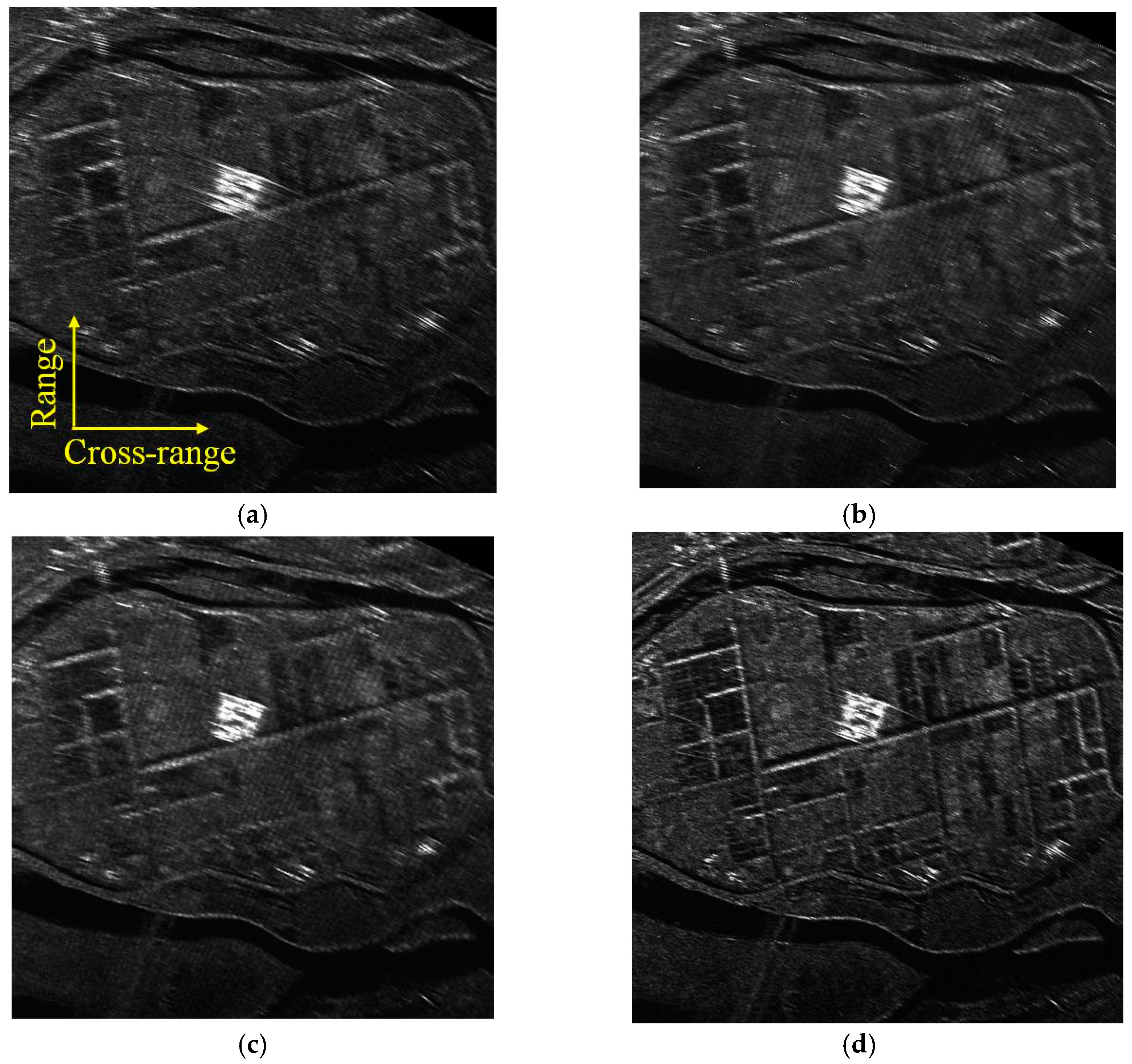
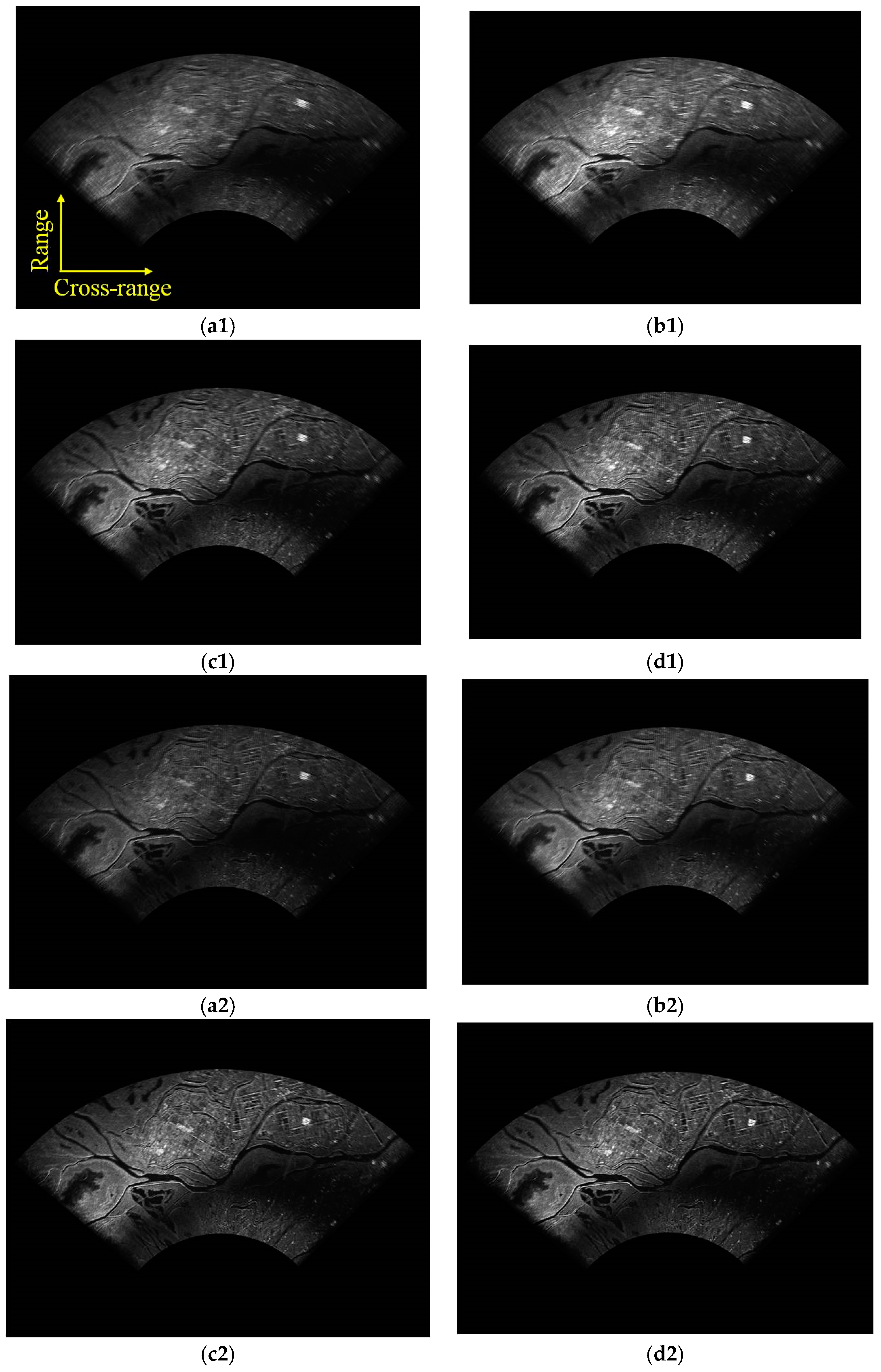
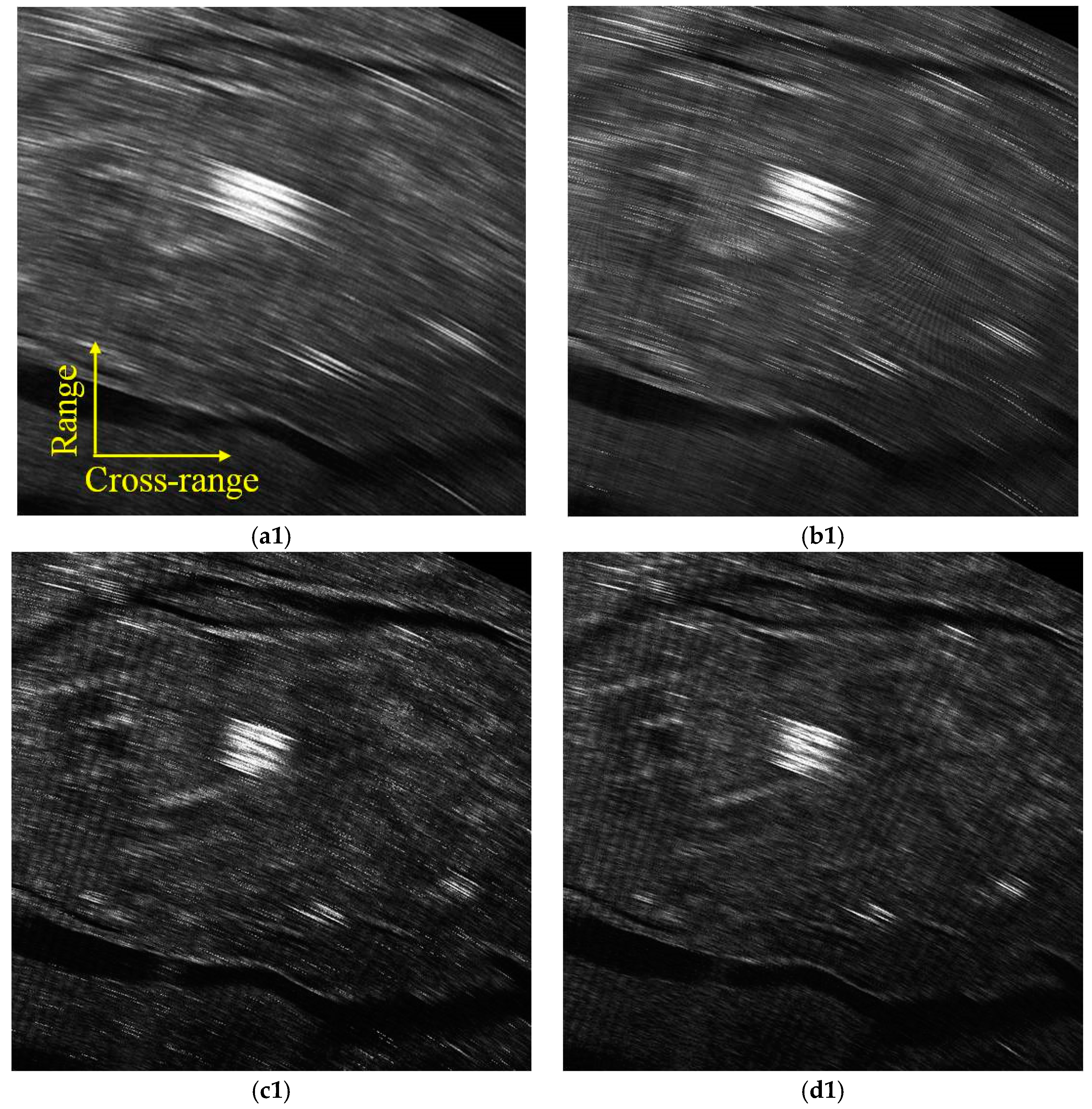
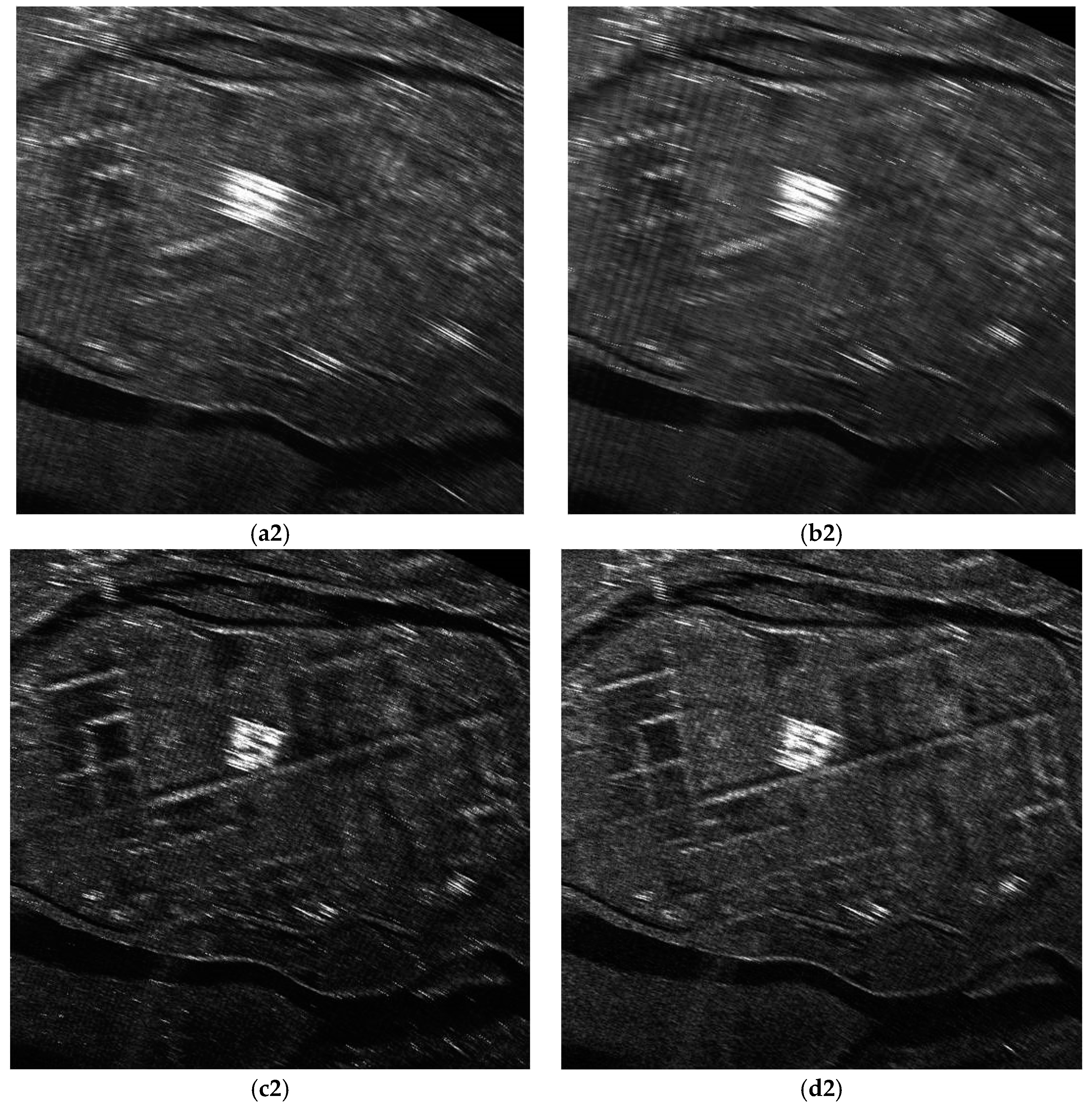
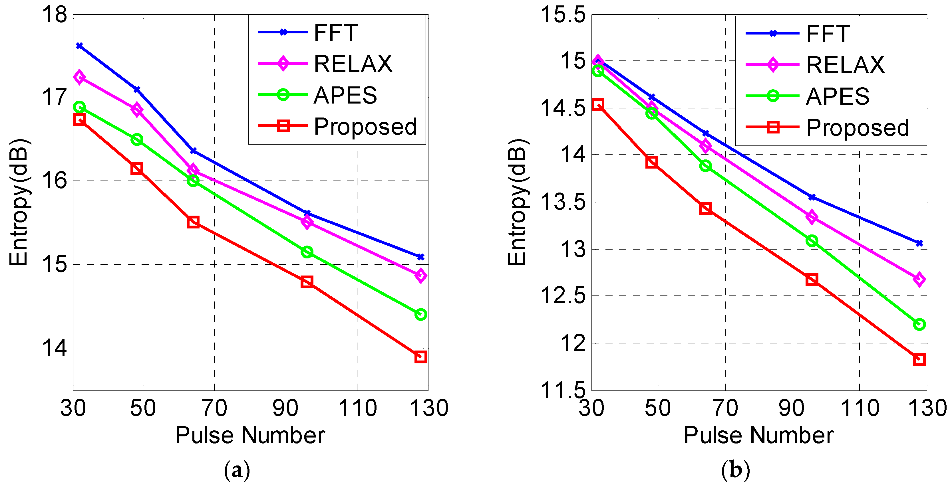
4.2. Real Data
5. Discussion
6. Conclusions
Author Contributions
Funding
Acknowledgments
Conflicts of Interest
References
- Cumming, I.G.; Wong, F.H. Digital Processing of Synthetic Aperture Radar Data: Algorithms and Implementation; Artech House: Norwood, MA, USA, 2005. [Google Scholar]
- Radant, M.E. The evolution of digital signal processing for airborne radar. IEEE Trans. Aerosp. Electron. Syst. 2002, 38, 723–733. [Google Scholar] [CrossRef]
- Brenner, A.R.; Ender, J.H.G. Demonstration of advanced recon-naissance techniques with the airborne SAR/GMTI sensor PAMIR. IEE Proc.-Radar Sonar Navig. 2006, 153, 152–162. [Google Scholar] [CrossRef]
- Cerutti-Maori, D.; Klare, J.; Brenner, A.R.; Ender, J.H.G. Wide-area traffic monitoring with the SAR/GMTI system PAMIR. IEEE Trans. Geosci. Remote Sens. 2008, 46, 3019–3030. [Google Scholar] [CrossRef]
- Yan, H.; Wang, R.; Li, F.; Deng, Y.; Liu, Y. Ground moving target extraction in a multichannel wide-area surveillance SAR/GMTI system via the relaxed PCP. IEEE Geosci. Remote Sens. Lett. 2013, 10, 617–621. [Google Scholar] [CrossRef]
- Wang, C.H.; Liao, G.S.; Zhang, Q.J. First spaceborne SAR-GMTI experimental results for the Chinese Gaofen-3 dual-channel SAR sensor. Sensors 2017, 17, 2683. [Google Scholar] [CrossRef] [PubMed]
- Zheng, M.; Yan, H.; Zhang, L.; Yu, W.; Deng, Y.; Wang, R. Research on strong clutter suppression for Gaofen-3 dual-channel SAR/GMTI. Sensors 2018, 18, 978. [Google Scholar] [CrossRef] [PubMed]
- Long, T.; Lu, Z.; Ding, Z.G.; Liu, L.S. A DBS Doppler centroid estimation algorithm based on entropy minimization. IEEE Trans. Geosci. Remote Sens. 2011, 49, 3703–3712. [Google Scholar] [CrossRef]
- Chen, H.; Li, M.; Lu, Y.; Wu, Y. A DBS image stitching algorithm based on affine transformation. In Proceedings of the IET Radar Conference, Xi’an, China, 14–16 April 2013; pp. 1–4. [Google Scholar]
- Cheng, Y.; Sun, C. Applications of superresolution signal estimators to Doppler beam sharpened imaging. J. Electron. 2000, 22, 392–397. [Google Scholar]
- Chen, H.M.; Li, M.; Lu, Y.L.; Zuo, L.; Zhang, P. Novel supper-resolution wide area imaging algorithm based on APES. Syst. Eng. Electron. 2015, 37, 6–11. [Google Scholar]
- Bamler, R.; Eineder, M. ScanSAR processing using standard high precision SAR algorithms. IEEE Trans. Geosci. Remote Sens. 1996, 34, 212–218. [Google Scholar] [CrossRef]
- Liang, C.; Fielding, E.J. Interferometry with ALOS-2 full-aperture ScanSAR data. IEEE Trans. Geosci. Remote Sens. 2017, 55, 2739–2750. [Google Scholar] [CrossRef]
- Prats, P.; Scheiber, R.; Mittermayer, J.; Meta, A.; Moreira, A. Processing of sliding spotlight and TOPS SAR data using baseband azimuth scaling. IEEE Trans. Geosci. Remote Sens. 2010, 48, 770–780. [Google Scholar] [CrossRef]
- Xu, W.; Huang, P.; Wang, R.; Deng, Y.; Lu, Y. TOPS-mode raw data processing using chirp scaling algorithm. IEEE J. Sel. Top. Appl. Earth Obs. Remote Sens. 2014, 7, 235–246. [Google Scholar] [CrossRef]
- Raney, R.K.; Runge, H.; Bamler, R.; Cumming, I.G.; Wong, F.H. Precision SAR processing using chirp scaling. IEEE Trans. Geosci. Remote Sens. 1994, 32, 786–799. [Google Scholar] [CrossRef]
- Chen, J.; Xing, M.; Sun, G.; Li, Z. A 2-D Space-variant motion estimation and compensation method for ultrahigh-resolution airborne stepped-frequency SAR with long integration time. IEEE Trans. Geosci. Remote Sens. 2017, 55, 6390–6401. [Google Scholar] [CrossRef]
- Wang, Y.; Li, J.W.; Sun, B.; Yang, J. A novel azimuth super-resolution method by synthesizing azimuth bandwidth of multiple tracks of airborne stripmap SAR data. Sensors 2016, 16, 869. [Google Scholar] [CrossRef] [PubMed]
- Mittermayer, J.; Moreira, A.; Loffeld, O. Spotlight SAR data processing using the frequency scaling algorithm. IEEE Trans. Geosci. Remote Sens. 1999, 37, 2198–2214. [Google Scholar] [CrossRef]
- Kay, S.M. Modern Spectral Estimation: Theory and Application; Prentice-Hall: Englewood Cliffs, NJ, USA, 1988. [Google Scholar]
- Kay, S.M.; Marple, S.L., Jr. Spectrum analysis-A modern perspective. Proc. IEEE 1981, 69, 1380–1419. [Google Scholar] [CrossRef]
- Gupta, I.J.; Beals, M.J.; Moghaddar, A. Data extrapolation for high resolution radar imaging. IEEE Trans. Antennas Propag. 1994, 42, 1540–1545. [Google Scholar] [CrossRef]
- Li, W.; Yang, J.; Huang, Y. Keystone transform-based space-variant range migration correction for airborne forward-looking scanning radar. Electron. Lett. 2012, 48, 121–122. [Google Scholar] [CrossRef]
- Moore, T.G.; Zuerndorfer, B.W.; Burt, E.C. Enhanced imagery using spectral-estimation-based techniques. Linc. Lab. J. 1997, 10, 171–186. [Google Scholar]
- Khorshidi, S.; Karimi, M.; Nematollahi, A.R. New autoregressive (AR) order selection criteria based on the prediction error estimation. Signal Process. 2011, 91, 2359–2370. [Google Scholar] [CrossRef]
- Giurcaneanu, C.; Saip, F.A.A. New insights on AR order selection with information theoretic criteria based on localized estimators. Digit. Signal Process. 2014, 32, 37–47. [Google Scholar] [CrossRef]


| Parameters | Value |
|---|---|
| Time width | 10 s |
| Band width | 12 MHz |
| Pulse repetition frequency | 2500 Hz |
| Azimuth beam width | 3.2° |
| Coherent pulses | 128 |
| Range gate number | 2048 |
| Parameters | Value |
|---|---|
| Time width | 24 us |
| Band width | 40 MHz |
| Pulse repetition frequency | 2500 Hz |
| Scanning area | 45°~135° |
| Coherent pulses | 128 |
| Range gate number | 4096 |
© 2019 by the authors. Licensee MDPI, Basel, Switzerland. This article is an open access article distributed under the terms and conditions of the Creative Commons Attribution (CC BY) license (http://creativecommons.org/licenses/by/4.0/).
Share and Cite
Chen, H.; Wang, Z.; Liu, J.; Yi, X.; Sun, H.; Mu, H.; Li, M.; Lu, Y. Knowledge-Aided Doppler Beam Sharpening Super-Resolution Imaging by Exploiting the Spatial Continuity Information. Sensors 2019, 19, 1920. https://doi.org/10.3390/s19081920
Chen H, Wang Z, Liu J, Yi X, Sun H, Mu H, Li M, Lu Y. Knowledge-Aided Doppler Beam Sharpening Super-Resolution Imaging by Exploiting the Spatial Continuity Information. Sensors. 2019; 19(8):1920. https://doi.org/10.3390/s19081920
Chicago/Turabian StyleChen, Hongmeng, Zeyu Wang, Jing Liu, Xiaoli Yi, Hanwei Sun, Heqiang Mu, Ming Li, and Yaobing Lu. 2019. "Knowledge-Aided Doppler Beam Sharpening Super-Resolution Imaging by Exploiting the Spatial Continuity Information" Sensors 19, no. 8: 1920. https://doi.org/10.3390/s19081920