Estimation of Two-Dimensional Non-Symmetric Incoherently Distributed Source with L-Shape Arrays

1
School of Automation, Northwestern Polytechnical University, Xi’an 710072, Shaanxi, China
2
Science and Technology on Combustion, Thermal-Structure and Internal Flow Laboratory, Northwestern Polytechnical University, Xi’an 710072, Shaanxi, China
3
Center for Optical Imagery Analysis and Learning, Northwestern Polytechnical University, Xi’an 710072, Shaanxi, China
*
Author to whom correspondence should be addressed.
†
These authors contributed equally to this work.
Sensors 2019, 19(5), 1226; https://doi.org/10.3390/s19051226
Submission received: 11 February 2019
/
Revised: 3 March 2019
/
Accepted: 6 March 2019
/
Published: 11 March 2019
(This article belongs to the Special Issue Recent Advances in Array Processing for Wireless Applications)
Abstract
:In the field of array signal processing, distributed sources can be regarded as an assembly of point sources within a spatial distribution. In this study, a two-dimensional (2D) non-symmetric incoherently distributed (ID) source model is proposed; we explore the estimation of a 2D non-symmetric ID source using L-shape arrays. The 2D non-symmetric ID source is established by modeling the angular power density function (APDF) as a Gaussian mixture model. Estimation of the non-symmetric distributed source is proposed based on the expectation maximization (EM) framework. The proposed EM iterative framework contains three steps in the process of each circle. Firstly, the nominal azimuth and nominal elevation of each Gaussian component are obtained from the phase parts of elements in sample covariance matrices. Then the angular spreads can be solved through a one-dimensional (1D) search by the original generalized Capon estimator. Finally, weights of each Gaussian component are obtained by solving the least-squares estimator. Simulations are conducted to verify the effectiveness of the estimation technique.
1. Introduction
In array signal processing, applications such as wireless communications, radar and underwater acoustics, point source models (assuming that signals impinging into receive arrays are from point sources) are commonly used, which can simplify calculations. In the real surroundings of radar and sonar systems, because of multipath propagation between receive arrays and targets, especially when the distances of targets and receive arrays are short, the spatial scatterers of targets cannot be ignored, assumptive condition of point source is no longer valid and point source models cannot characterize sources effectively, which should be described by distributed source models [1]. Distributed sources can be regarded as an assembly of point sources within a spatial distribution. The shape of spatial distribution is related to geometry and surface property of a target, for instance, in underwater detection. Considering multipath propagation and the surface feature of targets, distributed source models are more appropriate in near field of radar or sonar detection.
Distributed sources may be classified into coherently distributed (CD) sources or incoherently distributed (ID) sources [1]. Characterized by deterministic angular signal distribution function (ASDF) representing spatial distribution, CD sources assume that scatterers within a source are coherent. On the contrary, scatterers of an ID source are supposed to be uncorrelated. Spatial distributions of ID sources are characterized by angular power density function (APDF).
Spatial distribution of a distributed source, both ASDF and APDF, can be generally modeled as Gaussian, uniform or any other distribution. Parameters of ASDF and APDF contain nominal angles and angular spreads. Nominal angles can also be expressed as nominal direction-of-arrival (DOA) representing the center of targets. Nominal spreads denote the spatial extension of targets. Traditional estimation of a distributed source mainly involves estimation of DOA and angular spreads, which are implied in ASDF or APDF.
For CD sources, representative achievements of parameters estimation are deriving the rotation invariance relation with respect to different array configuration by virtue of Taylor series expansions [2,3,4,5,6,7,8,9]. Performance of distributed signal parameter estimator (DSPE) algorithm is analyzed in [10] and the performance of multiple signal classification (MUSIC) is analyzed in [11]. In this paper, the modeling and estimation of an ID source are considered.
Investigators for ID sources have been developed from classical point sources estimation techniques. DSPE [1] and dispersed signal parametric estimation (DISPARE) [12] have been developed from MUSIC, both of which involve a two-dimensional (2D) spectral search. In [13], an estimator extended from estimation of signal parameters via rotational invariance techniques (ESPRIT) has been proposed for ID sources, which use the total least square-ESPRIT (TLS-ESPRIT) algorithm to estimate the nominal DOAs of sources firstly, and then the angular spreads are estimated using the central moments of the distribution. Generalizations of Capon’s methods have been proposed in [14,15,16], which involve a two-dimensional (2D) spectral search besides a high-order matrix inversion. The maximum likelihood (ML) approach [17,18,19] has better accuracy but leads to a multidimensional nonlinear optimization requiring high computational complexity. Developed from least squares estimators, covariance matching estimation techniques (COMET) [20,21,22,23,24] have lower computational complexity than ML but with the same large sample behavior. Applying sparse representation to first-order Taylor expansion of steering vectors, in the case of small angular spreads, the authors of [25] proposed an estimator via block sparse Bayesian learning for multiple incoherently distributed sources, which has presented better accuracy under fewer snapshots.
The aforementioned methods consider sources as one-dimensional (1D) ID models, which have two parameters: the nominal DOA and angular spread. However, impinging signals and arrays sensors are not in the same plane practically. 2D distributed source models characterized by 2D DOA and 2D angular spread should be more reasonable, which usually contain four parameters: nominal azimuth, nominal elevation, azimuth angular spread and elevation angular spread. Including more parameters, there have been relatively few studies on estimation of 2D ID sources. The authors of [26] have proposed an extension of COMET for 2D ID sources, which employs alternating projection principle [27] and estimates 2D DOAs and 2D angular spreads separating source powers and noise variances to reduce complexity. Based on double parallel uniform linear arrays, the authors of [28] have proposed a TLS-ESPRIT like approach for 2D DOAs, where estimation of nominal elevations is firstly implemented via rotational invariance relations based on the diffused steering vectors derived from the first-order Taylor series expansions, then the nominal azimuth is estimated by 1D searching. Authors of [29] have proposed a (ESPRIT) like algorithm for 2D ID sources based on uniform rectangular arrays. Receive vectors of arrays in [29] are described by generalized steering vector, which is composed of nominal steering vector and its first-order partial derivatives along the direction of elevation and azimuth. Nominal angles are estimated through rotational invariance relations of generalized steering vectors, which are derived under the assumption of small angular spreads and small distance between sensors. Generally, DOA estimation of ID sources by virtue of diffused steering vectors or generalized steering vectors are derived from the first-order Taylor series expansions under the assumption of small angular spreads [26] or the assumption of both small angular spreads and small distance between sensors [28,29]. Though different methods based on different arrays have analyzed the influence of angular spreads of Gaussian or uniform ID sources on DOA estimation, what is a satisfactory accuracy respect to a real specific target has not been carried out until now. The assumption that distance between sensors is far less than wavelength of the signal is applicable to few specific detection areas, such as underwater low frequency detection.
All the distributed sources estimation techniques mentioned above assume that the shape of sources is symmetric. Nevertheless, scatterers are distributed irregularly within targets and the surface of targets is generally non-symmetric. Models of 1D non-symmetric ID sources have been proposed according to the principle that a non-symmetric distribution can be constructed by symmetric distributions. The authors of [30] have proposed a non-symmetric ID source model, where the shape of APDF can be figured via the variation of the ratio between two Gaussian distributions. The authors of [31] have employed the Gaussian mixture model to characterize the 1D non-symmetric ID sources and proposed a COMET algorithm embedded in expectation maximization (EM) framework [32,33] to estimate the 1D non-symmetric APDF. Containing more parameters, estimation for a non-symmetric ID source mainly lies in estimation of the non-symmetric APDF, which is different from estimation of a symmetric ID source.
To the best of our knowledge, there are no algorithms for 2D non-symmetric distributed sources. In this paper, we are concerned with modeling and estimation of a 2D non-symmetric ID source. As the principle that symmetric distributions can form a non-symmetric distribution is also true in the case of 2D, we present a 2D non-symmetric ID source model by constituting APDF with the 2D Gaussian mixture model. The authors of [34] have explored Cramer-Rao bound of L-shape arrays composed of two orthogonal ULAs and shown that such arrays have better accuracy potential than traditional cross arrays using same number of sensors with respect to point sources. Utilizing the propagator method, the authors of [35] have said that L-shape arrays composed of two orthogonal ULAs with less number of elements can estimate better than parallel shape arrays using the same method. Several DOA estimation methods [36,37,38,39] have been developed based on a point source model with L-shaped array placed in xoz or xoy plane. Estimation for a 2D non-symmetric ID source is proposed under EM framework based on L-shape arrays. The general EM framework is to get the best parameters by maximization of the likelihood function during the iteration process. As a 2D non-symmetric ID source has more parameters than those of an ID symmetric source; maximization of the likelihood function makes it difficult to apply for a 2D non-symmetric ID source because of nonlinear and high dimensional property. In our method, parameters are obtained successively in each EM cycle. Deducing the covariance matrices via the first-order Taylor series expansion of the steering vectors in each Gaussian component, we find that the nominal DOA parameters are related to the phase parts in elements of covariance matrices. Accordingly, nominal azimuth and nominal elevation of each Gaussian component can be obtained by the sample covariance matrices. Then angular spreads can be searched through the original Generalization of Capon’s estimator base on DOA parameters. Weights are estimated by a least squares fit of theoretical covariance and sample covariance.
The rest of this paper is organized as follows. Section 2 formulates a 2D non-symmetric ID source model and describes the received signal vectors and covariance matrix under L-shape array. Section 3 details the proposed algorithm of estimation for parameters of the 2D non-symmetric ID source. Section 4 shows numerical simulations to validate the proposed estimation method. Section 5 draws the conclusion of this paper.
2. Distributed Source Model
Figure 1 shows the L-shape arrays configuration, which uses the xoy plane. Array X is composed of sensors on x axis, while sensors on y axis constitute array Y. Each linear array consists of K sensor elements separated by d meters, and the two linear arrays share an origin sensor. Suppose that there is a stationary narrow-band 2D ID source with azimuth angle θ and elevation angle φ distributed in a spatial distribution. θ ∈ [0, π/2], φ ∈ [0, π/2]. λ is the wavelength of the signal impinging into the array sensors. The K × 1 dimensional received signal vectors of the arrays X and Y can be expressed as follows:
where (•)T denotes the transpose. xk(t) and yk(t) are the signal received by kth sensors in arrays X and Y, which can be expressed as follows:
An ID source means that different scatterers from one target generate uncorrelated multipath signals. s(t) in Equations (3) and (4) is the impinging signal into the target. L is number of scatterers. nxk(t) and nyk(t) are noises received. αl(t) is random complex ray gain of the lth scatterer. The random complex ray gain αl(t) is supposed to be white and independent from snapshot to snapshot as well as from scatterer to scatterer, which has the following relationship:
where |αl(t)|2 = σα/L, δ(•) is the Kronecker delta function, (•)* denotes the conjugate operator. Define nx(t) and ny(t), which are the K × 1 dimensional additive noise vectors of arrays X and Y; they can be written as:
nx(t) and ny(t) can be combined into
The noise is assumed to be uncorrelated with signal and uncorrelated between sensors as well as Gaussian white with zero mean:
where ρ is the power of noise, I2K is the 2K × 2K identity matrix, (•)H denotes the Hermitian transpose.
Combine x(t) and y(t) into:
The signal is assumed to be uncorrelated with the noise; the covariance matrix of z(t) can be written as follows:
The concept of APDF reflecting the distribution of scatterers of a source can be traced back to references [1] and [19], which can be approximately modeled as 2D Gaussian and uniform or any other distribution function according to the different characteristic of ID sources. Denote f(θ,φ) as APDF of an ID source. The (k,h)th noise free element of covariance matrix Rx is given by (proof can be seen in Appendix A):
where P = σα|s(t)|2 is the received power of the target. Define a(θ,φ) and b(θ,φ) are K × 1 dimensional steering vectors of arrays X and Y, which can be written as follows:
Thus, the covariance matrices Rx, Ry, Rxy and Ryx can be expressed as follows (proof is in Appendix B):
In this study, the Gaussian mixture model is used for angular power density of the distributed source in order to express the non-symmetric distribution, so the APDF of a non-symmetric ID source can be expressed as follows:
where the APDF consists of q Gaussian components g(θ,φ; ui) i= 1,2,…,q. ui = [,,,] is the parameter set of the ith Gaussian component denoting the nominal azimuth, nominal elevation, azimuth angular spread, and elevation angular spread, respectively.
To normalize f(θ,φ), the weighting coefficient wi satisfies the following constraint:
APDF in (17) can be shaped asymmetrically via the variation of the weighting coefficient wi and parameter set of each Gaussian component.
Combine a(θ,φ) and b(θ,φ) into:
The summation of Gaussian mixture distributions in Equation (17) can be substituted for f(θ,φ). Rz can be expressed respectively as follows:
Equation (16) can be expressed as follows:
where IK denotes the K × K identity matrix, denotes power of the ith Gaussian component.
3. Proposed Method
For a 2D non-symmetric ID source, there are 5q unknown parameters in APDF. Compared with a 2D symmetric source, there are many more parameters to be estimated. Traditional methods such as the maximum likelihood function, COMET, and the subspace-based algorithms are difficult applications, on account of the high dimensional property of the 2D non-symmetric ID source. In this section, based on EM framework and the alternating projection principle, an iterative algorithm is proposed, which contains three steps in each iterative cycle: first, the nominal elevation angle and nominal azimuth angle of each Gaussian component are obtained utilizing feature of covariance matrices; then angular spreads are estimated by 1D searching; finally, estimation of weights are implemented though a least squares fit of theoretical and sample covariance.
3.1. Latent Variable Model
On the basis of the latent variable model [32,33], the observed received vectors x(t) and y(t) caused by source and noise can be considered as a combination of unobserved received vectors caused by each Gaussian component implied in APDF of (17) as well as noise accompanying each Gaussian component. xi(t) and yi(t) are supposed to be the K × 1 dimensional implied received vectors of arrays X and Y, reflecting received signal impinged by the ith Gaussian component and the noise accompanying the ith Gaussian component. According to the latent variable model, x(t) and y(t) are the observed data, which can be assumed as incomplete data; xi(t) and yi(t) can be assumed as complete data. The many-to-one function representing the relationship of incomplete data and complete data can be expressed as follows:
Combine complete data xi(t) and yi(t) into:
Thus, we have a relationship of incomplete data z(t) and complete data zi(t) as follows:
According to the incoherently distributed source assumption, signals from different Gaussian component are uncorrelated; so different implied received vectors zi(t) are uncorrelated. Then covariance matrix of the incomplete data z(t), Rz is accordingly a summation of Rzi which is covariance matrix of the complete data zi(t)., Rz can be expressed as:
As zi(t) is caused by the ith Gaussian component and its accompanied noise, covariance matrix of the complete data Rzi, can be a written as:
where ρi is noise power of complete data zi(t). From Equations (22) and (23), we find that Rzi is composed of four parts—covariance matrix of the complete data xi(t) Rxi, covariance matrix of the complete data yi(t) Ryi, covariance matrix of the complete data xi(t) and yi(t) Rxyi, covariance matrix of the complete data yi(t) and xi(t) Ryxi, which means that:
Denote the normalized noise-free covariance matrix of complete data zi(t) as follows:
The noise is assumed to be distributed in complete data equally so covariance matrix of zi(t), Rzi expressed by Equation (26) can also be expressed as follows:
Rxi, Ryi, Ryxi and Ryxi can be expressed as follows:
Assuming that the angular spread of both azimuth and elevation in each Gaussian component is small, d/λ is set at 1/2; sinθsinφ and cosθsinφ can be approximated by the first term in the Taylor series expansions. Thus, elements in the normalized noise-free signal covariance matrix of Equation (30) can be expressed as follows (proof can be seen in Appendix C):
where [•]kh denotes the element of the kth row and the hth column in a matrix.
3.2. EM Algorithm
The EM algorithm is an iteration process containing two steps in turn: an expectation step (E-step) and a maximization step (M-step). The E-step serves to obtain parameters that are implied in each Gaussian component under the condition of incomplete data and the parameters values of E-step in the last EM circle. The M-step serves to update parameters based on the data from parameters obtained in the E-step, which is usually performed by maximizing the logarithm of the likelihood function.
The sample covariance matrix of incomplete data z(t), Rz can be replaced by with N snapshots, which is defined as follows:
, and are the estimated sample covariance matrix of complete data zi(t), xi(t) and yi(t). As is a sufficient statistic of unknown parameters wi, 𝜃i, 𝜙i, 𝜎𝜃i, 𝜎𝜙i and P, the (m+1)th E-step of the EM algorithm serves to calculate the expected value of sufficient statistics as follows (the proof can be seen in Appendix D):
where the superscript m indicates the value at the mth iteration.
To simplify the calculation, we assume the same angular spread for both azimuth and elevation =. The M-step will minimize the negative logarithm of the likelihood function to find the optimal parameters in the (m + 1)th iteration, which can be expressed as follows:
where parameters to be estimated are implied in Rzi which can be expressed by Equations (29)–(31). Equation (34) means exploring the best (m + 1)th parameters of the ith Gaussian component based on the sample covariance matrix of the complete data . Minimizing the Equation (34) is computationally complicated because of nonlinearity and inversion of the high-dimensional matrix; therefore, solving all the unknown parameters simultaneously is impossible. According to the principle of alternating projection, parameters can be estimated successively based on other parameters that have already been solved in M-step.
According to Equation (27), the sample covariance matrices of the complete data xi(t) and yi(t) can be obtained as follows:
where IK is the K × K identity matrix and 0K is K × K zero matrix.
From Equation (31), we show that the phase parts of the elements of rx(ui) and ry(ui) contain information of cosθisinφi and sinθisinφi, which means that we can obtain cosθisinφi and sinθisinφi from phase parts of Rxi and Ryi. Average phase parts of all elements in matrix and except the real diagonal elements, denote ηi as cosθisinφi and υi as sinθisinφi. Thus, we obtain:
where angle(•) denotes the phase of a complex number. Thus, we obtain θi and φi of the ith Gaussian component as:
After the nominal azimuth and nominal azimuth angle are solved, the angular spread of the ith Gaussian components can be estimated by using the original generalized Capon estimator:
where μmax(•) represents the maximal eigenvalue of a matrix.
The least-squares fit of the theoretical and sample covariance can be expressed as:
Differentiating Equation (42) with respect to Pi and ρ setting the results to zero yields the following equation:
At last, the weight of the ith Gaussian component can be obtained as follows:
After all parameters of the Gaussian component obtained in the (m + 1)th M-step, can be expressed by Equations (29)–(31). is the summation of according to Equation (25). Then the (m + 2)th iteration can be started.
3.3. Complexity Analysis and Comparison
Now, we analyze the computational complexity of the proposed method in comparison with COMET [26] and DISPARE [12], which are estimators for symmetric ID sources. It is noteworthy that the original algorithm in DISPARE [12] is for 1D ID sources and can be extended for 2D ID sources. COMET [26] is a method of estimation under alternating the projection algorithm framework; its computational cost mostly consists of calculation of the sample covariance matrix and the alternating projection technique with respect to cost functions. The DISPARE method estimates DOA and angular spreads through a three-dimensional (3D) spectrum-peak searching and its computation cost is mostly made of three parts: the calculation of the sample covariance matrix, the eigendecomposition of the matrix, and a 3D searching. The computation cost of the proposed method in one EM circle mainly consists of three operations: calculation of the 2K × 2K sample covariance matrix, 1D searching for angular spread, and calculation of weights. Assume that M is the EM iteration number. Table 1 shows the main computational costs of three methods. From Table 1, we can clearly see if computational cost of estimation for non-symmetric distributed source is significantly higher than that of symmetric distributed source.
The stopping criterion of the EM algorithm is when all the parameters are no longer changing [30,31]. We define the iterative variation of all parameters as:
where represents a parameter value in the mth iteration. When reaches a sufficiently small value, all parameters can be considered keeping stable.
Now, our algorithm can be summarized as follows
Step 1: Determine the number q of Gaussian components. Initialize P, wi, θi, φi, σi ( i = 1,2,…,q).
Step 2: Compute the sample covariance matrix of incomplete data using Equation (32).
Step 3: Repeat the following sub-steps for M times, which is a sufficiently large number or until the iterative variation of all parameters reaches the condition .
- Compute the sample covariance matrices of complete data , and using Equations (33), (35) and (36).
- Calculate the nominal azimuth and nominal elevation from Equations (37)–(40).
- Calculate using Equation (27) and search angular spread rough 1D search by Equation (41).
- Estimate the power of each component using Equation (39) and calculate weight of each component by Equation (44).
- Repeat sub-steps 1 to 4 for i = 1, 2, …, q.
- Superscript m = m + 1.
It is noteworthy that the distribution of a 2D non-symmetric ID source is unknown, so the true number of Gaussian components is unknown. Estimation is performed as q is an initial parameter, which needs to be set artificially. Step 1 can be considered as 0th iteration of the EM cycle. P0 is supposed to equal to , which can be set at a unit power. is set at a small value initially. can be set at 1/q. Then, can be obtained according to Equations (29)–(31). can be obtained from Equation (25). As the incomplete data z(t) is observed, can consequently be obtained from Equation (33).
4. Results and Discussion
In this section, we investigate the effectiveness of the proposed method though four simulation experiments. Assume that L-shape arrays have a configuration as in Figure 1 with sensors numbers K = 4 in both X and Y axis, d/λ is set at 1/2. SNR is defined as follows:
Root mean squared error (RMSE) is used to evaluate estimation performance. The RMSE of the nominal angle is defined as:
where and are the estimated nominal azimuth and estimated nominal elevation of the ID source, respectively. The superscript denotes the estimated parameters in th Monte Carlo run. Mc is the number of Monte Carlo simulations, which is 500. θ and φ are the true nominal azimuth and nominal elevation, respectively.
We define the value corresponding to the maximum point of the APDF as the nominal angle of the non-symmetric ID source. Nominal angle can be obtained through partial derivative of the estimated APDF, according to the property of continuous distribution.
In addition to investigation of nominal angles, estimation of the spatial distribution should be emphasized with respect to a non-symmetric distributed source. To evaluate the estimation of spatial distribution, the RMSE of distributed function is defined as follows:
where is the estimated APDF in th Monte Carlo run. In this section, we compare the performances of the proposed algorithm with two traditional estimators for ID sources, the COMET [26], which can be applied for any 2D arrays, and DISPARE [12], which can be extended for a 2D case. A 2D non-symmetric ID source with APDF is constructed as follows:
where g(a1,a2,a3) denotes a Gaussian component
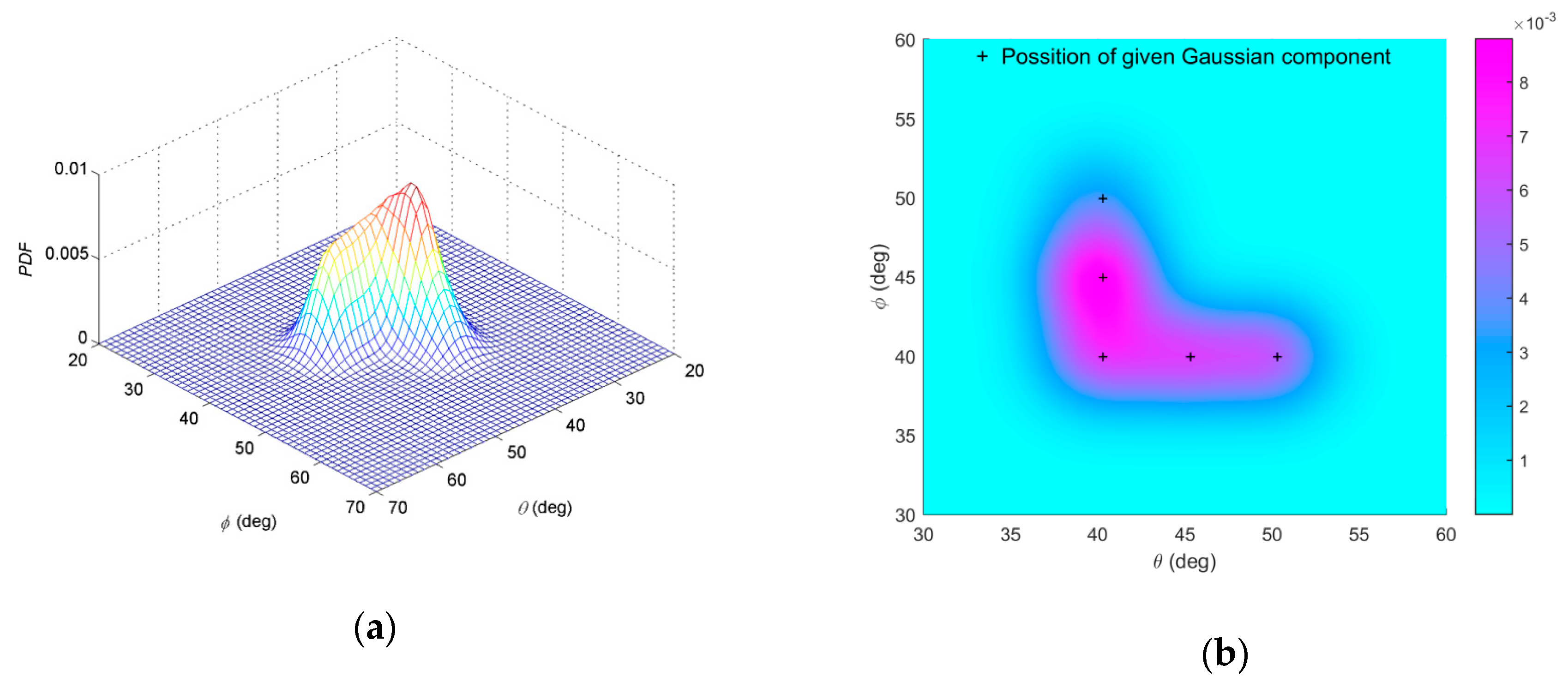
The nominal angle of the APDF can be calculated as (40°, 44.4°). Figure 2a,b shows the constructed non-symmetric APDF. The purple region of Figure 2b is projection of the constructed non-symmetric APDF on the θ-φ plane and the color bar represents measurement of probability density function (PDF). Mark + represents the central position of each Gaussian component in Equation (49).
When estimating a 2D non-symmetric ID source, we do not know details of the non-symmetric APDF. The proposed algorithm is performed by setting initial parameters of the Gaussian mixture and iterates until the parameters no longer change. The following experiments examine the parameter variety process of each Gaussian component, different experimental conditions, number of Gaussian components, and initial positions of Gaussian components. Effectiveness of the estimated APDF can be measured though RMSEa and RMSEf .
In the first example, the variety processes of Gaussian components in EM iterations are investigated. We choose four Gaussian components to estimate the source and set number of snapshots N = 200 and SNR = 15dB. As the shape of APDF of a 2D non-symmetric ID source to be estimated is unknown, we can firstly get DOA estimated by the traditional method, which is defined as an assumptive nominal angle of the 2D non-symmetric ID source. To be more representative, the initial positions of Gaussian components are set uniformly around the assumptive value with same distance to the assumptive nominal angle. Thus, the nominal azimuth and nominal elevation of four Gaussian components—A, B, C and D—are set uniformly around the value (47°,48.5°), estimated by DISPARE and set at (43°, 43°), (41.5°, 52.5°), (52.5°, 44.5°) and (51°, 54°) respectively, where the distances from initial Gaussian components to the assumptive nominal angle are all 6.8°. The initial angular spreads are set at 1°. Figure 3 shows the variety processes of parameters of each component. Figure 4 shows the initial and final values of each Gaussian component. The ordered array in parentheses (,,,, ) of Figure 4 is the parameters of the ith Gaussian component. The beginning of the arrow represents the initial value, while the end of the arrow is the final value. The final estimated APDF is:
The nominal angle of the APDF is (39.5°, 45.9°), which is near the nominal angle of the given sources. RMSEa is 1.58° and RMSEf is 0.29. The APDF is displayed in Figure 5, which reflects the spatial non-symmetric feature of the source and is similar to the given source. It is seen that parameters will converge to certain values as a result of sufficient EM iterations. A noticeable phenomenon wherein a small weight, 0.01, developed from component D whose central position is originally far from the given source, indicates that the initial Gaussian component outside the scope of the distributed source makes hardly any contribution to the final results.
In the second example, we investigate the influence of SNR and the number of snapshots N on the performance of the proposed algorithm in comparison with COMET and DISPARE. The RMSEa of the proposed algorithm and COMET, as well as DISPARE at different SNR and different number of snapshots N are shown, respectively, in Figure 6a,b, while RMSEf of three methods at different SNR and N are shown, respectively, in Figure 7a,b. The EM iteration number M is set at 500. We also choose four Gaussian components to estimate the unknown source. The distances from initial Gaussian components to the assumptive nominal angle of the source are all set at 6.8°. The initial angular spreads are set at 1°. Then we randomly choose four positions with equal interval around the assumptive nominal angle (47°, 48.5°) in each Monte Carlo run. Five hundred independent Monte Carlo simulations are run to obtain the results. The number of snapshots N is set at 200 in experiments shown in Figure 6a and Figure 7a, while the SNR is set at 15dB in experiments shown in Figure 6b and Figure 7b. As the number of snapshots N or SNR increases, all algorithms provide better performance. Apparently, the proposed algorithm provides higher estimation accuracy than COMET and DISPARE algorithm with regard to RMSEa and RMSEf. As can be shown in Figure 6a,b, RMSEa of COMET and DISPARE reach 4.3°, 4.3°, 7.1°, 7.3°. In Figure 7a,b, we have found that the RMSEf of COMET and DISPARE reach 1.08, 1.1, 2.1, 2.3. As to RMSEf, supposing in th Monte Carlo trail, if the estimated APDF = 0, = 1. RMSEfs estimated by COMET and DISPARE, are big errors considering distribution of function. Therefore, Figure 7a,b show that COMET and DISPARE is invalid as to the spatial distribution estimation of the given non-symmetric distributed source on account of the large errors of RMSEf.
In the third example, the influence of number of Gaussian components on performance is examined. The number of snapshots N = 200 and SNR = 15 dB. The initial angular spreads are set at 1°. When the performances of two or more Gaussian components are investigated, central positions of Gaussian components with equal interval around the assumptive nominal angle (47°, 48.5°) are randomly chosen in each Monte Carlo run; the distances from initial central positions to the assumptive nominal angle of the source are all set at 6.8°; 500 independent Monte Carlo simulations are run to obtain the result. As can be seen in Figure 8, the utilization of one Gaussian component provides a large error, which is an estimation considering sources as symmetric in essence. As the number of Gaussian components increase, RMSEf and RMSEa decrease. However, the final results of both RMSEf and RMSEa have little difference as the number changes from 3 to 6. Meanwhile, the convergence is markedly slower. It can be concluded that an increasing number of Gaussian components will provide a higher estimation accuracy, but the performance will not be notably improved as the number increase to a certain extent.
On the premise of not considering the cost of calculation, we can theoretically use any number of Gaussian components to fit a 2D non-symmetric ID source. In the third example, we examine the influence of different number of Gaussian components on estimation of a given source where the true number of Gaussian components is 5. It is found that the accuracy of estimation will not be significantly improved when q exceeds a certain extent. This phenomenon may be related to the shape of the given source. If the degree of asymmetry of the given 2D ID source is low, though it is composed of many Gaussian components, fewer Gaussian components can also fit the given 2D ID source well.
As the initial parameters of Gaussian components are set around assumptive value estimated by DISPARE or other methods for 2D symmetric sources, there will inevitably be Gaussian components with central positons outside the scope of the distributed source. To improve the robustness and accuracy of the algorithm, the number of Gaussian components should be set at a high level, and computing cost is also a matter of balance.
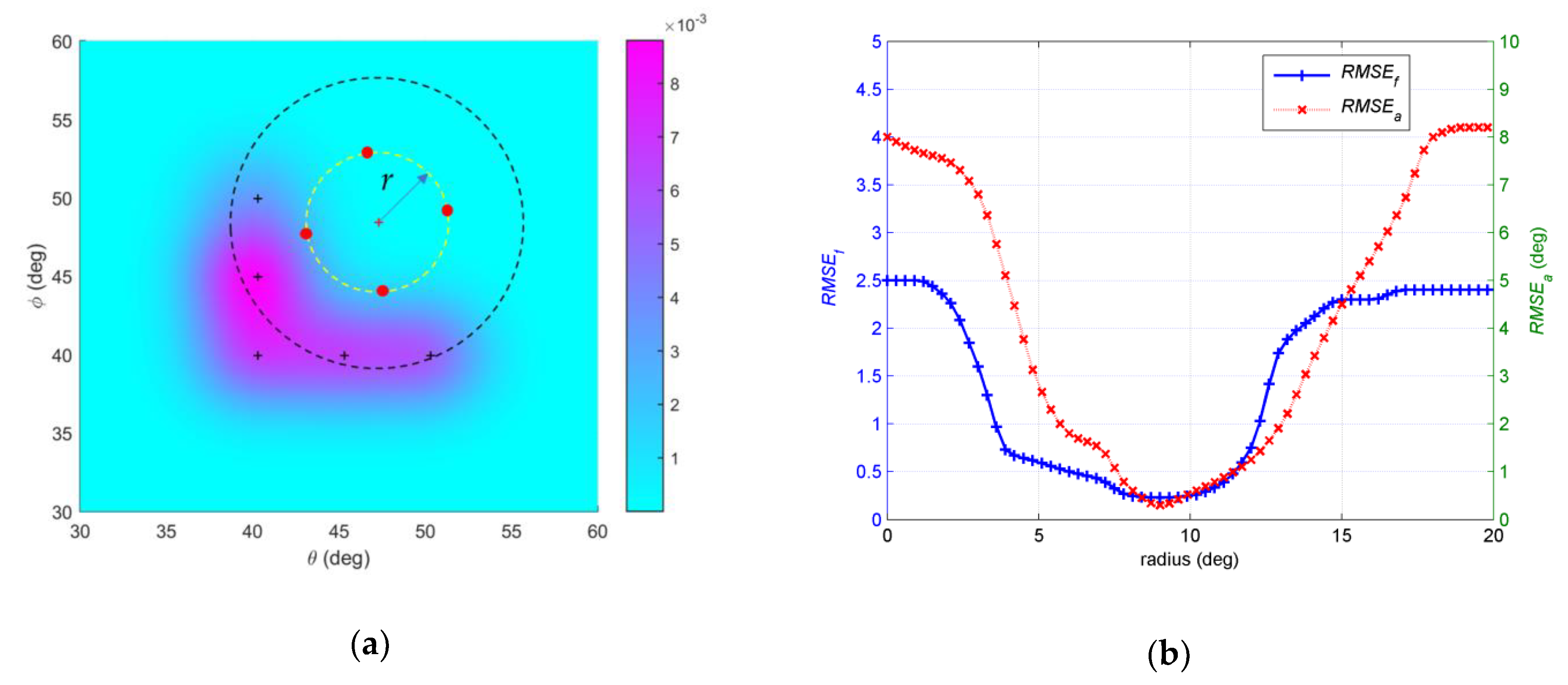
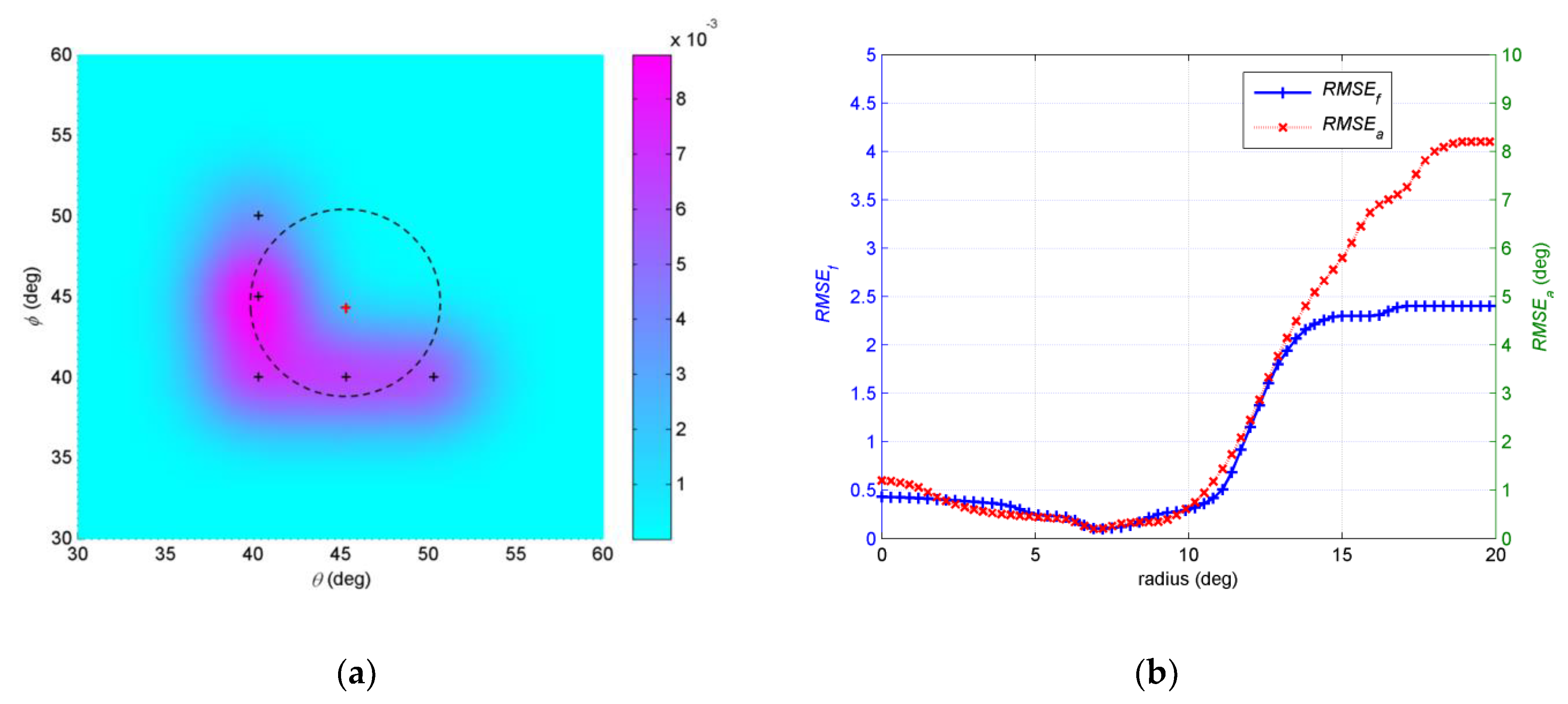
In the fourth example, we investigate the influence of initial positions to the final results. The number of snapshots N = 200 and SNR = 15dB. The initial angular spreads are set at 1°. The EM iteration is stopped under the condition Δ≤0.001. Three different assumptive nominal angles are considered. The first assumptive nominal angle is (47°,48.5°). Figure 9a shows that a circle is defined around the assumptive nominal angle (47°,48.5°). r is radius of the circle. We randomly select initial central positions of the Gaussian components, which are four points with equal interval on circle, such as the red dots in Figure 9a. 500 independent Monte Carlo simulations are run in a same circle, and then RMSEa and RMSEf are obtained with regard to each circle. We examine the radius of circle r changing from 0° to 20°. As shown in Figure 9b, both RMSEa and RMSEf change when the radius of the circle changes. The trends of the two curves are roughly the same. In general, as the radius increases, the estimation error decreases and then increases. When r is 8.5°, both RMSEa and RMSEf touch the bottom. The circle whose r equals 8.5° is drawn in dotted black line in Figure 9a. The second assumptive nominal angle is (45°, 44°), which is shown in Figure 10a. Setting process of initial positions is same as the first one. We examine the influence of radius of circle r changing on estimation. As shown in Figure 10b, both RMSEa and RMSEf decrease then increase with the radius of the circle increasing. The trends of the two curves are also roughly the same. When r is 6.8°, both RMSEa and RMSEf touch the bottom. The circle r equals 6.8° is drawn in dotted black line in Figure 10a. The third assumptive nominal angle is (50°, 42°), which is shown in Figure 11a. RMSEa and RMSEf changing with r are shown in Figure 11b. When r is 13.4°, both RMSEa and RMSEf touch the bottom. The circle r equals 13.4° is drawn in dotted black line in Figure 11a. The circles r, which equals 8.5°, 6.8° and 13.4° in the first, second and third trails, have common characteristics, such as initial positions of Gaussian components in these circles are within the given distributed sources with greater probability than any other circles. It is probable that estimation with initial positions of Gaussian components near the positions of Gaussian components in the given source has better accuracy than other parts, where the initial positions are far from the given source.
5. Conclusions
In this paper, we described the problem of estimating a 2D non-symmetric ID source based on L-shape arrays. The method we thus propose is developed by modeling the 2D non-symmetric APDF as a Gaussian mixture model. The estimation algorithm of a 2D non-symmetric ID source on the basis of iterative EM framework has been introduced in detail. The computational cost of a 2D non-symmetric ID source is much higher, when compared to the estimation of a 2D symmetric ID source. To evaluate the performance of estimation, we defined two indexes to reflect nominal angles and indicate spatial distribution. We investigated the parameter variety process of each Gaussian component, different SNR, number of snapshots, number of Gaussian components and initial positions of Gaussian components; the results of the numerical simulations show that the proposed method is effective for estimation of a non-symmetric ID source.
Author Contributions
Conceptualization, Z.D.; Methodology, T.W.; Software, T.W. and Z.L.; Writing—Original Draft Preparation, T.W. and Y.L.; Writing—Review & Editing, T.W. and Y.H.
Funding
This research was funded by the National Natural Science Foundation of China, grant numbers 61471299 and 51776222.
Acknowledgments
The authors would like to thank the editorial board and reviewers for the improvement of this paper.
Conflicts of Interest
The authors declare no conflict of interest.
Appendix A
Considering that the random complex ray gain of the lth scatterer αl(t) has a property described by Equation (5), as scatterers have density distribution f(θ,φ), when L is a large number, Equation (13) can be expressed as:
αl(t) is supposed to be white with zero mean and independent from snapshot to snapshot as well as from scatterer to scatterer. and , which is described by Equation (5). We can obtain:
Then [Rx]kh can be expressed as:
As f(θ,φ) is the density function of scatterers of a source, we have:
Then [Rx]kh can be expressed as:
Appendix B
Check Rx of Equation (16). According to Equation (14), the kth and hth elements of a(θ,φ) can be expressed as:
We can obtain:
From Equation (13), the (k,h)th noise free element of covariance matrix Rx can be expressed as . According to Equation (A9), the noise free [Rx]kh can be written as follows:
Considering the noise vector described by Equation (9), Rx can be expressed as follows:
The derivation processes of Ry, Rxy and Ryx is similar to Rx.
Appendix C
Check of Equation (27). Change variables for θ and for φ, where and are the small deviation of and . Thus, sinθsinφ and cosθsinφ can be approximated by the first term in the Taylor series expansions:
Appendix D
Assume that complete data zi(t) and incomplete data z(t) are zero-mean complex Gaussian random vectors and their covariance matrices are Rzi and Rz, respectively. According to the incoherently distributed source assumption, different vectors zi(t) are uncorrelated. Since z(t) is a linear combination of uncorrelated zi(t), the covariance matrix of zi(t) and z(t) can be written as follows:
Thus, the conditional expectation and variance of zi(t) under given observed data can be expressed as follows:
Thus, the conditional expectation of covariance matrix Rzi under the given observed data can be expressed as follows:
References
- Valaee, S.; Champagne, B.; Kabal, P. Parametric localization of distributed sources. IEEE Trans. Signal Process. 1995, 43, 2144–2153. [Google Scholar] [CrossRef]
- Wan, L.; Han, G.; Jiang, J.; Zhu, C.; Shu, L. A DOA Estimation Approach for Transmission Performance Guarantee in D2D Communication. Mobile Netw. Appl. 2017, 36, 1–12. [Google Scholar] [CrossRef]
- Dai, Z.; Cui, W.; Ba, B.; Wang, D.; Sun, Y. Two-Dimensional DOA Estimation for Coherently Distributed Sources with Symmetric Properties in Crossed Arrays. Sensors 2017, 17, 1300. [Google Scholar]
- Yang, X.; Zheng, Z.; Chi, C.K.; Zhong, L. Low-complexity 2D parameter estimation of coherently distributed noncircular signals using modified propagator. Multidim. Syst. Sign. P. 2017, 28, 1–20. [Google Scholar] [CrossRef]
- Zheng, Z.; Li, G.J.; Teng, Y. 2D DOA Estimator for Multiple Coherently Distributed Sources Using Modified Propagator. Circ. Syst. Signal Pr. 2012, 31, 255–270. [Google Scholar] [CrossRef]
- Zheng, Z.; Li, G.J.; Teng, Y. Low-complexity 2D DOA estimator for multiple coherently distributed sources. COMPEL. 2012, 31, 443–459. [Google Scholar] [CrossRef]
- Zoubir, A.; Wang, Y. Performance analysis of the generalized beamforming estimators in the case of coherently distributed sources. Signal Process. 2008, 88, 428–435. [Google Scholar] [CrossRef]
- Han, K.; Nehorai, A. Nested Array Processing for Distributed Sources. IEEE Signal Process. Lett. 2014, 21, 1111–1114. [Google Scholar]
- Yang, X.; Li, G.; Zheng, Z.; Zhong, L. 2D DOA Estimation of Coherently Distributed Noncircular Sources. Wireless Pers. Commun. 2014, 78, 1095–1102. [Google Scholar] [CrossRef]
- Xiong, W.; José, P.; Marcos, S. Performance analysis of distributed source parameter estimator (DSPE) in the presence of modeling errors due to the spatial distributions of sources. Signal Process. 2018, 143, 146–151. [Google Scholar]
- Xiong, W.; José, P.; Marcos, S. Array geometry impact on music in the presence of spatially distributed sources. Digit. Signal Process. 2017, 63, 155–163. [Google Scholar] [CrossRef]
- Meng, Y.; Stoica, P.; Wong, K.M. Estimation of direction of arrival of spatially dispersed signals in array processing. IET Radar Sonar Navig. 1995, 143, 1–9. [Google Scholar] [CrossRef]
- Shahbazpanahi, S.; Valaee, S.; Bastani, M. Distributed source localization using ESPRIT algorithm. IEEE Trans. Signal Process. 2001, 49, 2169–2178. [Google Scholar] [CrossRef]
- Xu, X. Spatially-spread sources and the SMVDR estimator. In Proceedings of the IEEE SPAWC’2003, Rome, Italy, 15–18 June 2003. [Google Scholar]
- Hassanien, A.; Shahbazpanahi, S.; Gershman, A.B. A generalized capon estimator for localization of multiple spread sources. IEEE Trans. Signal Process. 2004, 52, 280–283. [Google Scholar] [CrossRef]
- Zoubir, A.; Wang, Y. Robust generalised Capon algorithm for estimating the angular parameters of multiple incoherently distributed sources. IET Signal Process. 2008, 2, 163–168. [Google Scholar] [CrossRef]
- Raich, R.; Goldberg, J.; Messer, H. Bearing estimation for a distributed source: modeling, inherent accuracy limitations and algorithms. IEEE Trans. Signal Process. 2000, 48, 429–441. [Google Scholar] [CrossRef]
- Besson, O.; Vincent, F.; Stoica, P.; Gershman, A.B. Approximate maximum likelihood estimators for array processing in multiplicative noise environments. IEEE Trans. Signal Process. 2000, 48, 2506–2518. [Google Scholar] [CrossRef]
- Trump, T.; Ottersten, B. Estimation of nominal direction of arrival and angular spread using an array of sensors. Signal Process. 1996, 50, 57–69. [Google Scholar] [CrossRef]
- Besson, O.; Stoica, P. Decoupled estimation of DOA and angular spread for a spatially distributed source. IEEE Trans. Signal Process. 2000, 48, 1872–1882. [Google Scholar] [CrossRef]
- Shahbazpanahi, S.; Valaee, S.; Gershman, A.B. A covariance fitting approach to parametric localization of multiple incoherently distributed sources. IEEE Trans. Signal Process. 2004, 52, 592–600. [Google Scholar] [CrossRef] [Green Version]
- Zoubir, A.; Wang, Y.; Charge, P. On the ambiguity of COMET-EXIP algorithm for estimating a scattered source. In Proceedings of the IEEE International Conference on Acoustics, Speech, and Signal Processing, Philadelphia, PA, USA, 23–23 March 2005. [Google Scholar]
- Wen, C.; Shi, G.; Xie, X. Estimation of directions of arrival of multiple distributed sources for nested array. Signal Process. 2017, 130, 315–322. [Google Scholar] [CrossRef]
- Hassen, S.B.; Samet, A. An efficient central DOA tracking algorithm for multiple incoherently distributed sources. EURASIP J. Adv. Signal Process. 2015, 1, 1–19. [Google Scholar] [CrossRef]
- Yang, X.; Li, G.; Zheng, Z. Parameter estimation of incoherently distributed source based on block sparse Bayesian learning. In Proceedings of the IEEE International Conference on Digital Signal Processing, Singapore, 21–24 July 2015. [Google Scholar]
- Boujemâa, H. Extension of COMET algorithm to multiple diffuse source localization in azimuth and elevation. Eur. Telecommun. 2012, 16, 557–566. [Google Scholar] [CrossRef]
- Ziskind, I.; Wax, M. Maximum Likelihood Localization of Multiple Sources by Alternating Projection. IEEE Trans. Acoust. Speech Signal Process. 1988, 36, 1553–1560. [Google Scholar] [CrossRef]
- Zhou, J.; Li, G.J. Low-Complexity Estimation of the Nominal Azimuth and Elevation for Incoherently Distributed Sources. Wireless Pers. Commun. 2013, 71, 1777–1793. [Google Scholar] [CrossRef]
- Tao, W.; Zhenghong, D.; Yiwen, L. Two-dimensional DOA estimation for incoherently distributed sources with uniform rectangular arrays. Sensors 2018, 18, 3600. [Google Scholar]
- Kikuchi, S.; Tsuji, H.; Sano, A. Direction-of-arrival estimation for spatially non-symmetric distributed sources. In Proceedings of the IEEE International Conference on Sensor Array and Multichannel Signal Processing Workshop, Barcelona, Spain, 18–21 July 2004. [Google Scholar]
- Wang, H.; Li, S.; Li, H. Gaussian mixture model approximation of total spatial power spectral density for multiple incoherently distributed sources. IET Signal Process. 2013, 7, 306–311. [Google Scholar] [CrossRef]
- Moon, T.K. The expectation-maximization algorithm. IEEE Signal Proc. Mag. 1996, 6, 47–60. [Google Scholar] [CrossRef]
- Miller, M.I.; Fuhrmann, D.R. Maximum-likelihood narrow-band direction finding and the EM algorithm. IEEE Trans. Acoust. speech Signal Process. 1990, 37, 1560–1577. [Google Scholar] [CrossRef]
- Hua, Y.; Sarkar, T.K.; Weiner, D. L-shaped array for estimating 2-D directions of wave arrival. IEEE Trans. Antenn. Propag. 1991, 39, 143–146. [Google Scholar] [CrossRef]
- Tayem, N.; Kwon, H. L-shape 2-dimensional arrival angle estimation with propagator method. IEEE Trans. Antennas Propag. 2005, 53, 1622–1630. [Google Scholar] [CrossRef]
- Kikuchi, S.; Tsuji, H.; Sano, A. Pair-matching method for estimating 2-D angle of arrival with a cross-correlation matrix. IEEE Antennas Wireless Propag. Lett. 2006, 5, 35–40. [Google Scholar] [CrossRef]
- Liang, J.; Liu, D. Joint Elevation and Azimuth Direction Finding Using L-Shaped Array. IEEE Trans. Antennas Propag. 2001, 58, 2136–2141. [Google Scholar] [CrossRef]
- Wang, G.; Xin, J.; Zheng, N. Computationally Efficient Subspace-Based Method for Two-Dimensional Direction Estimation With L-Shaped Array. IEEE Trans. Signal Process. 2011, 59, 3197–3212. [Google Scholar] [CrossRef]
- Xi, N.; Liping, L.; Xi, N. A Computationally Efficient Subspace Algorithm for 2-D DOA Estimation with L-shaped Array. IEEE Signal Process. Lett. 2014, 21, 971–974. [Google Scholar]
Figure 1.
The L-shape arrays configuration.

Figure 2.
(a) Probability density function of APDF of the constructed non-symmetric ID source; (b) projection of the APDF on the θ−φ plane.
Figure 2.
(a) Probability density function of APDF of the constructed non-symmetric ID source; (b) projection of the APDF on the θ−φ plane.

Figure 3.
(a) The variety process of nominal azimuths in EM iterations; (b) the variety process of nominal elevations in EM iterations; (c) the variety process of angular spreads in EM iterations; (d) the variety process of weights in EM iterations.
Figure 3.
(a) The variety process of nominal azimuths in EM iterations; (b) the variety process of nominal elevations in EM iterations; (c) the variety process of angular spreads in EM iterations; (d) the variety process of weights in EM iterations.

Figure 4.
The initial and final values of each Gaussian component.

Figure 5.
The estimation of non-symmetric APDF by the proposed method.

Figure 6.
(a) RMSEa estimated by the three methods versus SNR; (b) RMSEa estimated by the three methods versus number of snapshots.
Figure 6.
(a) RMSEa estimated by the three methods versus SNR; (b) RMSEa estimated by the three methods versus number of snapshots.

Figure 7.
(a) RMSEf estimated by the three methods versus SNR; (b) RMSEf estimated by the three methods versus number of snapshots.
Figure 7.
(a) RMSEf estimated by the three methods versus SNR; (b) RMSEf estimated by the three methods versus number of snapshots.

Figure 8.
(a) RMSEa estimated by different number of Gaussian components; (b) RMSEf estimated by different number of Gaussian components.
Figure 8.
(a) RMSEa estimated by different number of Gaussian components; (b) RMSEf estimated by different number of Gaussian components.

Figure 9.
(a) Description of initial positions of Gaussian components and circles r equals 8.5°; (b) RMSEa and RMSEf estimated by different r with assumptive nominal angle (47°, 48.5°).
Figure 9.
(a) Description of initial positions of Gaussian components and circles r equals 8.5°; (b) RMSEa and RMSEf estimated by different r with assumptive nominal angle (47°, 48.5°).

Figure 10.
(a) Description of assumptive nominal angle (45°, 44°) and circles r equals 6.8°; (b) RMSEa and RMSEf estimated by different r with assumptive nominal angle (45°, 44°).
Figure 10.
(a) Description of assumptive nominal angle (45°, 44°) and circles r equals 6.8°; (b) RMSEa and RMSEf estimated by different r with assumptive nominal angle (45°, 44°).

Figure 11.
(a) Description of assumptive nominal angle (50°, 42°) and circles r equals 13.4°; (b) RMSEa and RMSEf estimated by different r with assumptive nominal angle (50°, 42°).
Figure 11.
(a) Description of assumptive nominal angle (50°, 42°) and circles r equals 13.4°; (b) RMSEa and RMSEf estimated by different r with assumptive nominal angle (50°, 42°).


Table 1.
Computational complexity of different methods.
| Method | Calculation of the Sample Covariance Matrix | Searching/AP Algorithm | Eigendecomposition/Calculation of Weights | Total |
|---|---|---|---|---|
| Proposed | o (4 NK2) + o(4 MK3) | o(8 MK3) | o(8 MK3) | o (64 MK3) + o (4 NK2) |
| COMET | o (4 NK2) | o (24 K3 + 12 K2) | o (24 K3 + 12 K2) + o (4 NK2) | |
| DISPARE | o (4 NK2) | o (24 K2+6 K) | o (8K3) | o (8 K3) + o (4 NK2) + o (24 K2 + 6 K) |
© 2019 by the authors. Licensee MDPI, Basel, Switzerland. This article is an open access article distributed under the terms and conditions of the Creative Commons Attribution (CC BY) license (http://creativecommons.org/licenses/by/4.0/).
Share and Cite
MDPI and ACS Style
Wu, T.; Deng, Z.; Li, Y.; Li, Z.; Huang, Y. Estimation of Two-Dimensional Non-Symmetric Incoherently Distributed Source with L-Shape Arrays. Sensors 2019, 19, 1226. https://doi.org/10.3390/s19051226
AMA Style
Wu T, Deng Z, Li Y, Li Z, Huang Y. Estimation of Two-Dimensional Non-Symmetric Incoherently Distributed Source with L-Shape Arrays. Sensors. 2019; 19(5):1226. https://doi.org/10.3390/s19051226
Chicago/Turabian StyleWu, Tao, Zhenghong Deng, Yiwen Li, Zhengxin Li, and Yijie Huang. 2019. "Estimation of Two-Dimensional Non-Symmetric Incoherently Distributed Source with L-Shape Arrays" Sensors 19, no. 5: 1226. https://doi.org/10.3390/s19051226
Note that from the first issue of 2016, this journal uses article numbers instead of page numbers. See further details here.