A Novel Link-to-System Mapping Technique Based on Machine Learning for 5G/IoT Wireless Networks


Department of Electronics Engineering, Chungnam National University, Daejeon 34134, Korea
*
Author to whom correspondence should be addressed.
Sensors 2019, 19(5), 1196; https://doi.org/10.3390/s19051196
Submission received: 15 December 2018
/
Revised: 19 February 2019
/
Accepted: 5 March 2019
/
Published: 8 March 2019
(This article belongs to the Special Issue Scalable and Efficient Networking and Communication Architectures in IoT Domain)
Abstract
:In this paper, we propose a novel machine learning (ML) based link-to-system (L2S) mapping technique for inter-connecting a link-level simulator (LLS) and a system-level simulator (SLS). For validating the proposed technique, we utilized 5G K-Simulator, which was developed through a collaborative research project in Republic of Korea and includes LLS, SLS, and network-level simulator (NS). We first describe a general procedure of the L2S mapping methodology for 5G new radio (NR) systems, and then, we explain the proposed ML-based exponential effective signal-to-noise ratio (SNR) mapping (EESM) method with a deep neural network (DNN) regression algorithm. We compared the proposed ML-based EESM method with the conventional L2S mapping method. Through extensive simulation results, we show that the proposed ML-based L2S mapping technique yielded better prediction accuracy in regards to block error rate (BLER) while reducing the processing time.
1. Introduction
With technological advance of 4G LTE/LTE-A (Long Term Evolution-Advanced) cellular communications, the number of wireless smart devices has increased explosively. Wireless smart devices have being applied in various services such as IoT (Internet of Things) communications, autonomous vehicles communication, augmented reality service, etc. [1]. In the near future, a wide range of service requirements will be demanded due to advent of many use cases [2]. However, 4G LTE/LTE-A systems have several limitations to satisfy requirements of various services.
As the next version of 4G LTE/LTE-A, 3GPP Release 15 (Rel-15) has specified 5G new radio access (NR) and core technologies from December 2017 and it is known as 5G NR. 5G NR access technology is evolving to support a variety of service requirements and it contains enhanced mobile broadband (eMBB), massive machine type communications (mMTC), and ultra reliable low latency communications services (URLLC) as 5G representative services [3]. To support low latency service, 5G NR system has embraced new flexible frame structures different from 4G LTE/LTE-A system with a fixed sub-carrier interval. Moreover, to support high data rate and high traffic service for eMBB use cases, 5G NR systems are expanding to high frequency bands above 6 GHz. Accordingly, 5G NR system will be mainly operated on high frequency band with a wide bandwidth [4].
In a wide band channel, a transport block (TB) is allocated into N narrow band channels and each narrow band channel goes through a different fading condition on its own sub-carrier. Therefore, user equipment (UE) experiences different post-processing signal to interference plus noise ratio (SINR) over every sub-carrier. In a traditional narrow band channel, block error rate (BLER) is estimated from a curve of mean SINR and mean BER. On the contrary, in the wide band channel, different N post-processing SINRs are mapped to the averaged post-processing SINR. Since the concept of the averaged post-processing SINR is defined as an effective SNR, this many-to-one mapping is called an effective SNR mapping (ESM) technique. Besides, ESM technique is used for the purpose of physical layer abstraction when evaluating a system-level simulator (SLS). A simplified link-level simulator (LLS) helps SLS reduce complexity of computation and it can help improve a simulator performance. Since the concept of a physical level abstraction for SLS is reflected, this is also called a link-to-system (L2S) mapping technique. Accordingly, a L2S mapping is that post-processing SINRs extracted from LLS are mapped to an effective SNR and BLER is predicted by the effective SNR, thus, it is called effective SNR mapping (ESM).
In prior studies, many researchers analyzed exponential effective SINR mapping (EESM) [5,6] and mutual information based ESM [7] as representative L2S mappings. In [8], effective SNR is analyzed on the side of uplink. In [9], impact of L2S is analyzed on the side of system level. However, there are too many data extracted from LLS as well as too much processing time is need to find EESM mapping parameters for various cases. Moreover, loss incurs due to an inaccuracy from additive white Gaussian noise (AWGN) curve of SNR and BLER.
Therefore, recently, researchers studied ML-based link abstraction models. In [10], support vector machine is used to enable ML classification for fast adaptive modulation coding. This scheme exploits measurement of single TB success or failure to train the classifier. In [11], a ML method based on a logistic regression is proposed. To predict a TB success or failure, their basic model uses mean and standard deviation of the SINR set, modulation rate, and TB size as input variables. To improve the estimation accuracy, adding terms of higher order or combinations of input variables are used in an enhanced model.
To utilize ML-based link abstraction models that have been studied thus far, ML algorithms should be applied on both of an evolved Node-B (eNB) and UE sides. However, since the number of UEs is too large, it is difficult to embed ML algorithms in all UEs. Some UEs can directly apply ML algorithms while other UEs should take the existing EESM method. Therefore, eNBs still need the existing EESM method. In our previous work [12], we proposed a ML-based EESM method where training data are learned by deep neural network (DNN) regression and L2S mapping based on EESM is executed by optimization algorithms under 4G LTE system environments. We showed that the processing time and accuracy are improved. However, L2S mapping-related previous studies including our previous work have been done based on 3G/4G cellular networks. Our previous work is meaningful as the existing results under SISO condition of 4G LTE systems are applied to machine learning techniques.
Recently, the standards of 5G NR systems based on Rel-15 decided that LDPC channel coding on data plane is preferred and clustered delay line (CDL) and tapped delay line (TDL) as 5G channel models are used. Since the standards of 5G NR based on Rel-15 are continually progressing, the performance results for AWGN channel of simple model are not easy to obtain. To develop LLS, SLS, and network-level simulator (NS) for 5G NR based on Rel-15, a Korean collaborative research project developed 5G K-Simulator during August 2016–February 2019 [13,14]. Our role was to develop a L2S mapping method as an inter-connection between the LLS and the SLS in 5G K-Simulator. To the best of our knowledge, were were the first to design a machine learning based L2S mapping under 5G NR systems based on Rel-15. The main contributions of this paper are as follows:
- (1)
- AWGN curves based on 5G NR system are provided. In conventional L2S mapping schemes, an AWGN curve is required to estimate block error rate (BLER) on SLS. We provide the AWGN curve of SNR-BLER under 5G NR systems and compare the AWGN curves of SNR-BLER between 4G LTE system and 5G NR systems.
- (2)
- The values of SNR satisfying at a target BLER = 0.1 (10%) are provided through AWGN curve. 3GPP 4G LTE and 5G NR-standards are specified to set the target BLER of 0.1, i.e., 10%. In SLS, signal-to noise ratio (SNR) can be measured immediately, but the calculation of BLER is burden because CRC decoding has to be performed. When a measured BLER is lower than the target BLER, UE can change to the index of higher CQI to support high data rate. Therefore, we provide the values of SNR thresholds under an unknown BLER satisfying the target BLER of 0.1 through the simulation results.
- (3)
- The methodology for 5G NR L2S mapping is provided based on ML. The optimal parameters for L2S mapping depend on a given environment. In addition, 5G NR systems have flexible frame structures. Therefore, we provide the methodology for 5G NR L2S mapping based on ML to extract the data for any cases and find the optimal mapping parameters.
- (4)
- The optimal mapping parameters for L2S mapping are provided in SISO and 2 × 2 MIMO cases under given conditions.
This paper is organized as follows. In Section 2, we introduce 5G NR system and main difference of 4G and 5G systems. In Section 3, we describe the methodology for 5G NR L2S mapping. In Section 4, we propose machine learning-based effective SNR mapping procedure. In Section 5, we validate the proposed scheme and show the simulation results of the proposed scheme. Finally, we draw conclusions in Section 6. The abbreviations commonly used in this paper are summarized as Table 1.
2. Background on 5G NR
3GPP Rel-15 was approved for NR standards in December 2017, referred to as 5G NR. Different from 4G LTE-A systems with fixed sub-carrier intervals, 5G NR systems have newly flexible frame structures to provide various services. Various transmission frame settings are available by introducing sub-carrier interval parameter called numerology. 5G NR systems can set from 0 to 5, and the value of determines the sub-carrier interval. As the numerology value increases by one, the sub-carrier interval is doubled. Compared to 5G NR systems, 4G LTE/LTE-A systems only use a fixed sub-carrier interval of 15 kHz (), therefore, it can accommodate various services.
The most innovative change of 5G NR system is channel coding. Turbo codes [15], low-density parity-check (LDPC) code [16], and polar code [17] were designated as candidate channel codings. In particular, LDPC code and the polar code have been actively studied, and the performance of LDPC code has been shown to be close to the Shannon limit. In a recent study, LDPC code enables fast encoding/decoding with high error correction capability, and achieves high speed, low delay, low cost, and high reliability for 5G communication services. At the first-phase of Rel-15, LDPC code replaces the Turbo code used in 4G LTE data channels, while Polar code replaces the Tail Biting Convolutional Codes used in 4G LTE control channels.
3GPP standards technical reports of TR 38.900 [18] and TR 38.901 [19] define clustered delay line (CDL) and tapped delay line (TDL) as 5G channel models for LLS. Each channel model consists of three non-line-of-sight channels of A, B, and C types and two line-of-sight channels of D and E types. These channel models support bandwidth of up to 2 GHz in the 500 MHz to 100 GHz operating frequency.
The CDL model [18,19] is designed as a signal arriving at the receiver antenna dispersed into 20 signals as it passes through each cluster in the channel. At this time, the delay, power, and four kinds of angles (azimuth angles of arrival and departure, and zenith angles of arrival and departure) are defined. In the case of the TDL model, instead of defining each cluster parameter in the channel as in the CDL model, only the power delay profile of each taps is defined for the entire channel. Therefore, it is a simplified form in which the four angular values do not appear, and the process of distributing signals passing through each cluster to 20 signals is not modeled. It is also possible to generate TDL models by assuming non-isotropic antennas such as directive horn antennas or array antennas. The TDLs and the spatial-filtered TDLs can be used with the correlation matrices for MIMO link-level simulations.
In contrast, 4G LTE-A system models the wideband characteristics of the channel as a TDL. Each tap independently experiences a fading characteristic by an azimuth direction of departure and direction of arrival angular spectrum. Since the mean direction and angular spread are fixed, TDL represents stationary channel conditions in 4G LTE-A system.
3. Methodology for 5G NR Link-to-System Mapping
5G K-Simulator [13] is a Korean collaborative research project consisting of several Korean universities and companies to develop a 5G NR simulator. At the start of the project, there was no widely accepted L2S mapping suitable for 5G NR system. Our role was to develop a L2S mapping method as an inter-connection between the LLS and the SLS in 5G K-Simulator. In this section, we deal with considerations for the 5G NR system in Section 3.1, and we describe the preliminary phase to be performed in the LLS simulation for L2S mapping in Section 3.2. Finally, we explain a L2S mapping method for 5G NR systems in Section 3.3.
3.1. System Configuration/Setup
5G NR systems have been studied in many test scenarios in 3GPP TR 38.802 [20]. However, this paper focuses on parameter settings for L2S mapping test among many scenarios. Table 2 summarizes the system parameters used in this paper, and details are described below.
- (1)
- Waveform: Although several candidate waveforms for uplink were proposed, Rel-15 recently decided to use OFDM-based waveforms with cyclic prefix for 5G NR downlink and uplink.
- (2)
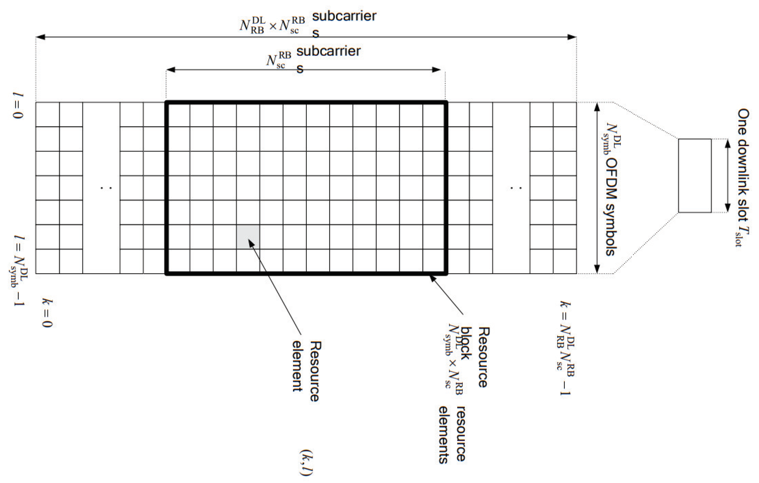
- Bandwidth and sub-carrier spacing: The size of resource blocks (RBs) is determined by the product of the number of sub-carriers on the frequency-axis and the number of symbols on the time-axis, as shown in Figure 1 [21]. Bandwidth is set to 5 MHz in this paper. The maximum number of available RBs is 25 at bandwidth of 5 MHz. When sub-carrier spacing is applied to 15 kHz, 12 sub-carriers are allocated in one RB on the frequency-axis and 14 symbols are allocated per sub-frame on the time-axis. A sub-frame consists of two slots and one slot consists of seven symbols. Assuming that the full band of 5 MHz is assigned to UE, 4200 resource elements (REs) can be allocated to UE for one sub-frame since 4200 REs are calculated by 25 RBs × 12 sub-carriers × 7 symbols × 2 slots per sub-frame. In other words, one RE is equivalent to the minimum resource for a symbol time on the time-axis and a sub-carrier on the frequency-axis.
- (3)
- Channel coding: 5G NR replaces the previously used Turbo-code to LDPC coding. The number of the information bits and the number of the encoded bit are varied depending on channel coding schemes, the number of RBs, and the modulation scheme. TB size represents the number of information bits that can be transmitted throughout 4200 REs and it is denoted as A. After encoding TB of length A by channel coding scheme, the output is to be encoded bits of length E. Table 3 summarizes values of A and E according to the turbo code and LDPC when using 25 RBs per sub-frame. denotes modulation order and its values are 2, 4, and 6 for QPSK, 16QAM, and 64QAM, respectively.
- (4)
- Channel model: Ideally, transmit signal is transferred over AWGN channel after LDPC encoding and rate matching. In practice, we experimented with fading channel environments in which CDL-A and TDL-A are utilized in SISO and 2 × 2 MIMO environments.
3.2. Preliminary Phase for 5G NR L2S Mapping
To perform L2S mapping, data of post-processing SINRs corresponding to allocated REs and BLERs is required. The procedure to extract raw data of post-processing SINRs and BLER from LLS is considered as a preliminary phase for L2S mapping. In AWGN environment, methods to extract raw data for L2S mapping are almost the same as the performance evaluation of stand-alone LLS. However, methods to extract raw data for L2S mapping in the fading channel environment are different from existing LLS evaluation methods. The preliminary phase for 5G NR L2S mapping is discussed in this subsection.
We consider fading channel models such as CDL or TDL specified in 3GPP TR 38.900 under downlink. As mentioned in Section 3.1, 4200 symbols are transmitted through 4200 REs for a sub-frame. Whenever one TB is generated every sub-frame, 4200 received SNRs corresponding 4200 REs can be measured on a UE side. Since a wide bandwidth of 5 MHz is used, the channel is varying on the frequency-axis domain but it does not change much on the time-axis. Therefore, we consider the received signal of 300 sub-carriers (i.e., 25 RBs × 12 sub-carriers × 1 symbol = 300 REs) at the first symbol-time to eliminate redundancy and reduce calculation complexity.
The received signal from the kth sub-carrier () at the first symbol-time in a sub-frame is expressed as follows:
where is a received signal vector on the kth sub-carrier, is the MIMO channel matrix on the kth RE, is the precoder matrix on the kth sub-carrier, is a transmitted symbol vector on the kth sub-carrier, and is a Gaussian noise vector on the kth sub-carrier. denotes the number of transmit antenna and denotes the number of receiver antennas.
A receiver filter on the kth sub-carrier by zero-forcing (ZF) and minimum mean square error (MMSE), , is given as follows:
where denotes a receiver filter matrix, and denotes the number of spatial transmission layers.
The estimated received symbol vector on the kth sub-carrier by a receiver filter, , is expressed as follows:
where .
Post-processing SINR of the kth sub-carrier at the mth layer is calculated as follows:
where is a signal in row m and column i of matrix. The numerator term is the desired signal at the mth layer, whereas the first term of denominator is the sum of the inter-stream interference signals and the second term is the filtered noise.
Since each layer is independent and identically distributed, in the case of a large number of simulation, it does not matter to collect raw data from how many layers or which layer. For simplicity of experiment, raw data of post-processing SINRs and BLER is collected at the first layer. Accordingly, the variable m can be replaced to a constant 1 with the meaning of the first layer, and then it can be removed. Consequently, Equation (4) can be expressed to Equation (5) as follows:
In a SISO case, m, , , and set to be 1, and there is no inter-stream interference. Thus, the post-processing SINR at the kth sub-carrier is expressed as follows:
For convenience of expression, post-processing SINRs () is denoted by .
One thousand TBs are repeatedly transmitted for a given input SNR under the same channel condition. CRC error checking is applied to determine whether the TB is successfully decoded. UE transmits ACK by successful TB decoding among transmitted TBs, whereas it transmits NACK by failed decoding. Therefore, BLER is calculated as follows:
At the next input SNR under the same channel, 1000 TBs are transmitted recurrently. Correspondingly, the data of (, ⋯, , BLER) is collected for a given input SNR and REs where is the number of allocated sub-carriers per symbol, i.e., 300. Thus, raw data of (input SNR, , ⋯, , ) is gathered for L2S mapping. We describe LLS procedure to extract raw data as shown in Algorithm 1. Especially, the condition of channel must not be changed during the generation of 1000 TBs over all SNRs, while the condition of channel is changed at every simulation. The input SNR should be adjusted so that values of BLER are measured within the range of 0.01 and 0.9. When the value of measured BLER with 0 is used, is to be negative infinite, as shown in Equation (9). BLER with 1 is meaningless data since all TBs failed. Since MSE is calculated from measured BLERs, MSE is dependent by measured BLERs. The exact value of L2S mapping can not be derived if the BLER value does not appear evenly in BLER range from 0.01 to 0.9. Therefore, equally distributed BLERs within the range from 0.01 to 0.9 should be measured to find the values of L2S mapping parameters.
3.3. Schematic of 5G NR L2S Mapping
L2S mapping method has two aims to map various SNRs over allocated REs to one averaged SNR as well as to reduce system overload in SLS. The overall procedure of the L2S mapping is shown in Figure 2 where L2S mapping method basically receives raw data of and from the LLS and then delivers two mapping parameters of (, ) and 5G NR AWGN to the SLS. Our L2S mapping is composed of four modules: , loading raw data; , AWGN curve; , Effective SNR (ESM); and , exponential ESM (EESM) L2S mapping. The operation and function of each module are explained below.
- (1)
- Module : Loading raw datamodule reads stored data on the preliminary phase in Section 3.2. The format of raw data is composed of x rows and y columns for each CQI. The value of x is the number of input × the number of simulations () and the value of y is +2. As mentioned in Section 3.1, the number of allocated sub-carriers per sub-frame is . The first column is a given input SNR, the last column is , and the rest of columns mean , ⋯, . The data loading is performed for AWGN channel and all fading channels, respectively.
- (2)
- Module : AWGN curvemodule only applies to AWGN channel. It gets AWGN raw data from module and makes AWGN fitting curve for SNR versus BLER in the range of all CQIs. The AWGN fitting curve is generated from the relation of (, ⋯, ) and . Generally, the fitting curve is induced from an exponential function or regression curve of machine learning.
- (3)
- Module: Effective SNRmodule calculates an effective SNR applying and when a UE measures , and it is expressed as follows [5,6]:where and are determined after optimization in .In fact, SLS only measures without decoding. To estimate error for a received TB, SLS calculates an effective SNR from Equation (8) using and . The values of and are already reported to SLS through a L2S mapping method.
- (4)
- Module : EESM based L2S Mappingmodule finds optimal mapping parameters of and for a given CQI and a channel type. After performing M snapshots, we calculate mean square error (MSE) as follows [5,6]:where M denotes the total number of simulated snapshots and denotes the BLER measured from the ith post-processing SINR values. In addition, is calculated by Equation (8) at the ith snapshot, and is the value of BLER on AWGN channel. Furthermore, denotes output corresponding to input x from AWGN fitting curve. (It is plotted in module )To find optimal and , we minimize MSE for the entire range of (, ) as follows:Since the BLERs vs. SNR varies depending on the modulation method, code block size and code rate, we should find and for a given condition.
| Algorithm 1: Extract raw data. |
 |
4. Machine Learning Based Effective SNR Mapping Procedure
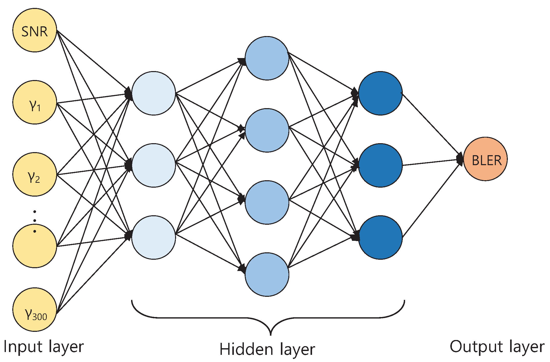
The number of simulations was 10,000 for each input SNR and each CQI and 1000 TBs were generated for each simulation. BLER was determined for transmitted 1000 TBs. Thus, the size of raw data of (, , ) to collect from LLS, i.e., the total number of simulation results per CQI was the product of the number of SNR values and the the number of simulations. In general, since the size of raw data from the LLS is large, obtaining the optimal parameters of and through heuristic search with Equation (10) is burdensome. Thus, it was necessary to reduce the computation complexity as well as to improve the accuracy. As shown in this section, we used Python Tensorflow framework and applied the DNN regression method to make an AWGN fitting curve of module in Section 3.3. The algorithm of DNN regression is described in Algorithm 2 and Figure 3.
- (1)
- We utilized the DNN regression method instead of the best fitting curve to obtain the BLER curve in AWGN channels. The DNN consists of several hidden layers between the input and output layers. Hidden layers of (100, 200, 100) layers were used in Adagrad optimizer [22]. As the number of hidden layers and the number of nodes at each hidden layer increased, MSE decreased. However, the improvement of MSE was saturated at three hidden layers with the number of nodes of (100, 200, 100), as shown in Figure 3. Learning rate was set to , which implies how quickly it is tuned to the target SNR value. The regularization strength to prevent over-fitting was set to . The sigmoid function was used as an activation function in hidden layers.
- (2)
- DNN regression continued training for SNRs and BLERs on AWGN channel with the learning rate at each epoch. The number of training data was 4000.
- (3)
- After training data, BLERs were predicted for test set of SNRs. Finally, we obtained an enhanced AWGN curve of SNRs and BLERs.
| Algorithm 2: DNN regression. |
| /* Configure DNN regression */ 1 regressor = learn.DNNRegressor(feature_columns, hidden_units = [100, 200, 100], optimizer = tf.train.ProximalAdagradOptimizer( learning_rate = 0.1, l1_regularization_strength = 0.001), activation_fn = tf.nn.sigmoid) /* Train measured data up to 4000 times */ 2 input_training_fn ← (awgn_snr, awgn_bler) 3 regressor.fit(input_fn = input_training_fn, steps = 4000) /* Predict of BLERs for test SNRs */ 4 input_reff_fn ← snr range 5 predictions = list(regressor.predict_scores(input_fn = input_reff_fn)) 6 regressed_bler = np.asarray(predictions) |
Next, we applied the optimization algorithm to efficiently find , which is summarized in Algorithm 3.
- (1)
- To find the optimal parameters , we loaded raw data from module in Section 3.2.
- (2)
- In the ML scheme, the loss function is defined as the difference between the calculated effective SNR value from Algorithm 3 and AWGN SNR obtained from Algorithm 2 at the same BLER. We calculated loss as the expectation of loss function over BLERs. The loss function and MSE of Equation (9) were used almost synonymously.
- (3)
- We applied optimization algorithms, Adagrad and RMSProp, to find the optimal parameters that minimize the loss function. Since Adagrad and RMSProp adapt the learning rate to the parameters, they eliminate the need to manually tune the learning rate. Adagrad optimizer adapts the learning rates by scaling them inversely proportional to the sum of the historical squared values of the gradient. In contrast, RMSprop optimizer modifies AdaGrad for a nonconvex setting by changing gradient accumulation into exponentially weighted moving average [23].
- (4)
- With the optimal parameters, the mean squared error (MSE) was calculated by
| Algorithm 3: Find optimal and . |
| /* Load data on Fading channel ; */ 1 snr_k ← post-processing SINRs, bler ← BLER /* Calculate with and */ 2 snr_eff = -1 * alpha1 * tf.log(tf.reduce_mean (tf.exp(-1*snr_k/alpha2), axis = 1)) /* Decide target SNR by regression */ 3 target_snr ← predicted snr corresponding to BLER /* Calculate loss function */ 4 loss = tf.reduce_sum(tf.abs(tf.subtract (target_snr,snr_eff))) /* Select a training algorithm between Adagrad and RMSprop; Adagrad is selected in this case. */ 5 train = tf.train.AdagradOptimizer(0.1).minimize(loss) /* train = tf.train.RMSPropOptimizer(0.1).minimize(loss) ← when RMSProp is selected. */ /* Training data 4000 times */ 6 with tf.Session() as sess: 7 sess.run(init) 8 for i in range(4000): 9 sess.run(train) /* Calculate MSE in test data set */ 10 regressed_bler ← estimated BLER, y_data ← BLER 11 mse = np.mean(np.square(np.subtract(np.asarray(y_data), np.asarray(regressed_bler)))) |
5. Numerical Results and Analysis
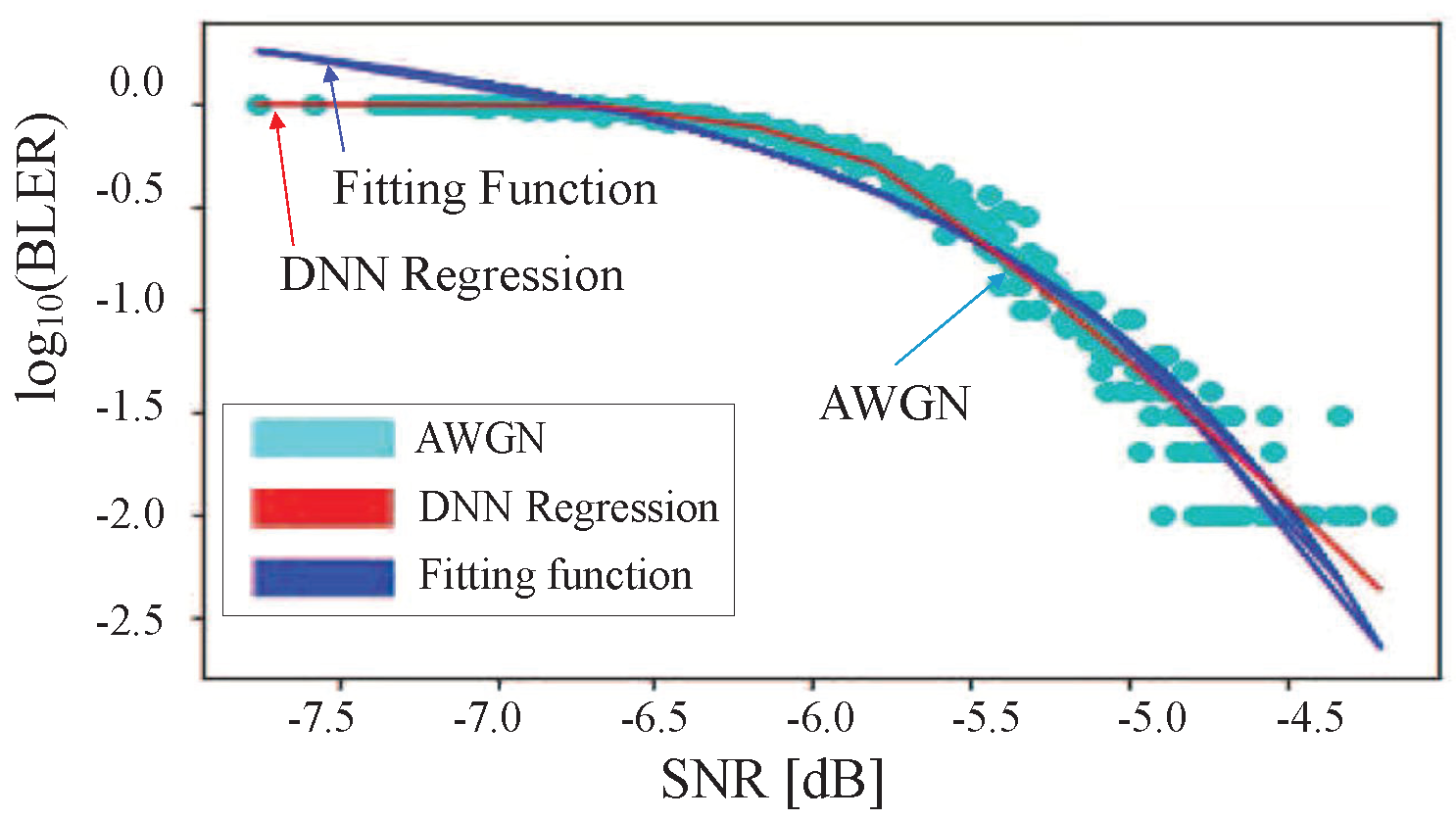
Table 2 shows the system parameters used. To make AWGN curve, we used a DNN regression method. Actually, we already showed that a DNN regression is a more suitable method than a fitting function under 4G LTE-A systems in our previous work [12]. The fitting curve became over-fitted as BLER approached zero, as shown in Figure 4. In contrast, a DNN regression followed AWGN curve as closely as possible through a multi-dimensional mapping. Moreover, Table 4 shows MSE results for fitting function (“FIT”) and DNN regression (“DNN”) for all CQIs under 4G LTE-A systems. Actually, the deep neural network gave little improvement compared to fitting algorithm under AWGN channel condition since AWGN was an almost static channel environment. Accordingly, in this study, 5G NR AWGN curve was generated with a DNN regression method without comparison of FIT and DNN.
5.1. AWGN Curve
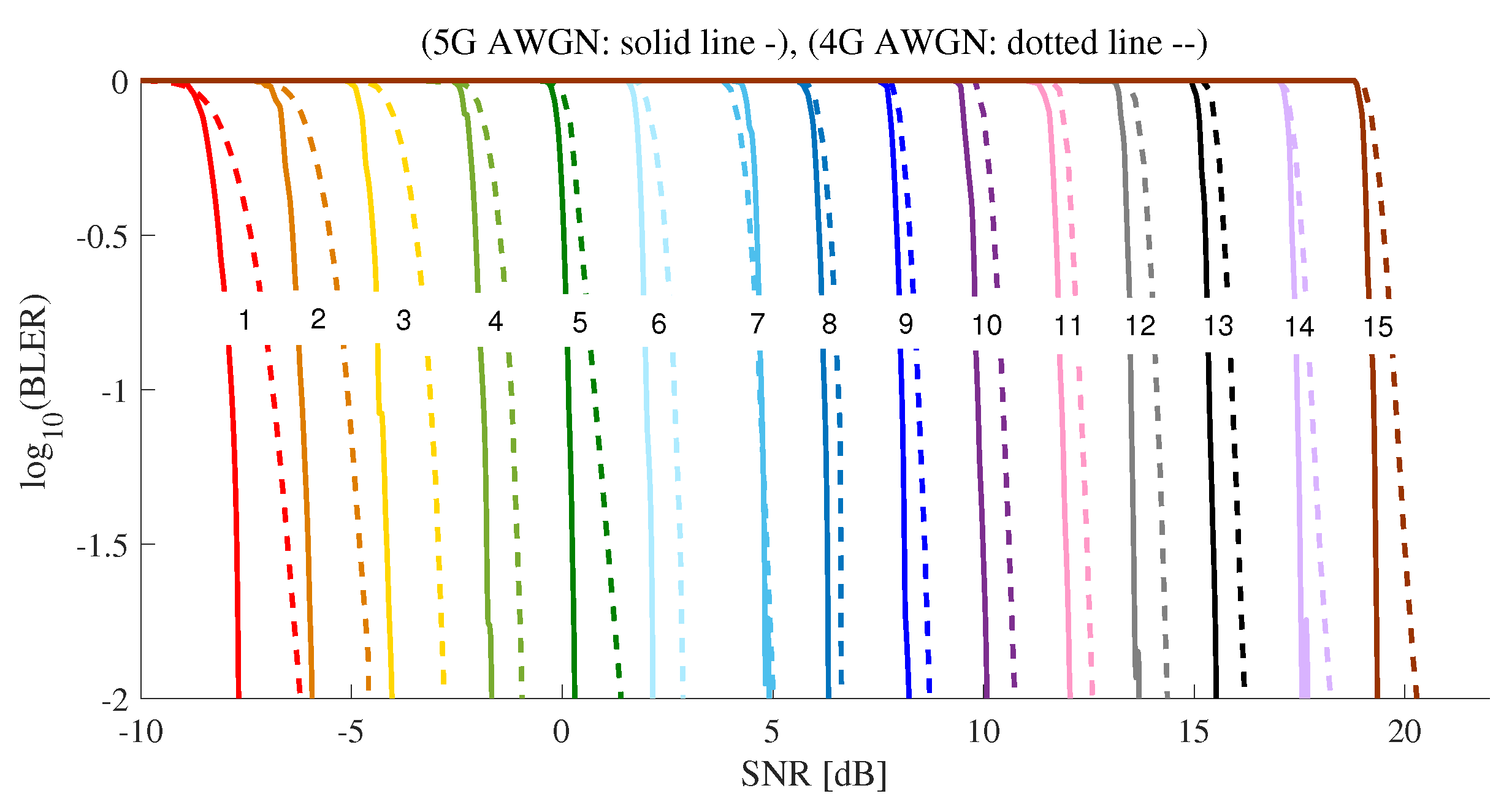
Figure 5 shows BLER performance for 4G AWGN and 5G AWGN. 4G LTE-A systems and 5G NR systems use Turbo-code and LDPC as channel coding schemes, respectively. The size of TB and their coding rates varied slightly according to channel coding schemes, as shown in Table 3. After applying the channel coding shown in Table 3, the performances of 4G AWGN and 5G NR AWGN were evaluated. 5G NR AWGN outperformed 4G AWGN, especially better for small CQL values.
3GPP 4G LTE and 5G NR-standards are specified to set the target BLER of 0.1, i.e., 10%. As SNR increased, BLER decreased. SNR could be measured immediately on SLS, but the calculation of BLER was burdensome because CRC decoding had to be performed. When measured BLER is lower than target BLER, a UE can choose the index of high CQI to support high data rate. Under an unknown BLER, we found the value of SNR satisfying the target BLER of 0.1 through the simulation results and induced Equation (12) for CQI and SNR.
From the AWGN curve shown in Figure 4, SINR threshold at BLER = 0.1 (10%) can be derived, as shown in Table 5. In practical 4G/5G systems, if an estimated BLER exceeds 0.1, TB transmission is considered as failure. Otherwise, TB transmission is considered as success. We plot SINR threshold at BLER = 10% for the range of all CQIs in Figure 6. From this plot, we derive a linear equation as follows:
where i means CQI index. is SINR threshold for CQI index i at 10% BLER.
5.2. Optimal Values of and
To find optimal values of and , two optimizers, Adgrad and RMSProp, were used. Table 6 shows optimal parameters in the case of 5G CDL-A SISO, whereas Table 7 shows optimal parameters in the case of 5G TDL-A 2 × 2 MIMO. The MSE performances of both optimizers were similar. In our previous work [12], we analyzed the optimal EESM parameters in 4G LTE-A system. At that time, the MSE performance of RMSProp was better than that of AdaGrad. However, since 5G NR AWGN curve aws too steep, there was little difference in performance of the two optimizers. In the case of 2 × 2 MIMO, the variance of was larger than that of SISO, thus the MSE of MIMO was larger than MSE of SISO.
5.3. Simulation Validation
Figure 7 and Figure 8 show the results of effective SNR mapping by the proposed ML-based EESM method in the case of 5G CDL-A SISO. “CQI1_SNR_k”, “CQI5_SNR_k”, “CQI10_SNR_k”, and “CQI15_SNR_k” indicate the post-processing SINRs , as mentioned in Equation (6). Since the number of allocated REs was 300 (25 RB × 12 sub-carriers × 1 symbol time = 300 REs), corresponding to are plotted in Figure 7. When wide-band signal passed through a fading channel, each RE suffered different fading. Thus, the results show that s spread widely. AWGN indicates SNR and BLERs at CQI 1, 5, 10 and 15 in 5G NR AWGN, as shown in Figure 5. To perform EESM L2S mapping, we applied optimal parameters of and obtained using RMSProp optimizer, as shown in Table 6. Blue mark presents effective SNRs and the results show that widespread were mapped to one effective SNR on the AWGN curve. Figure 8 shows how well is the effective SNR mapped to the AWGN for all CQIs. The results show that most blue marks were on the AWGN line. With these results, we observed that the proposed method predicted the BLER quite well.
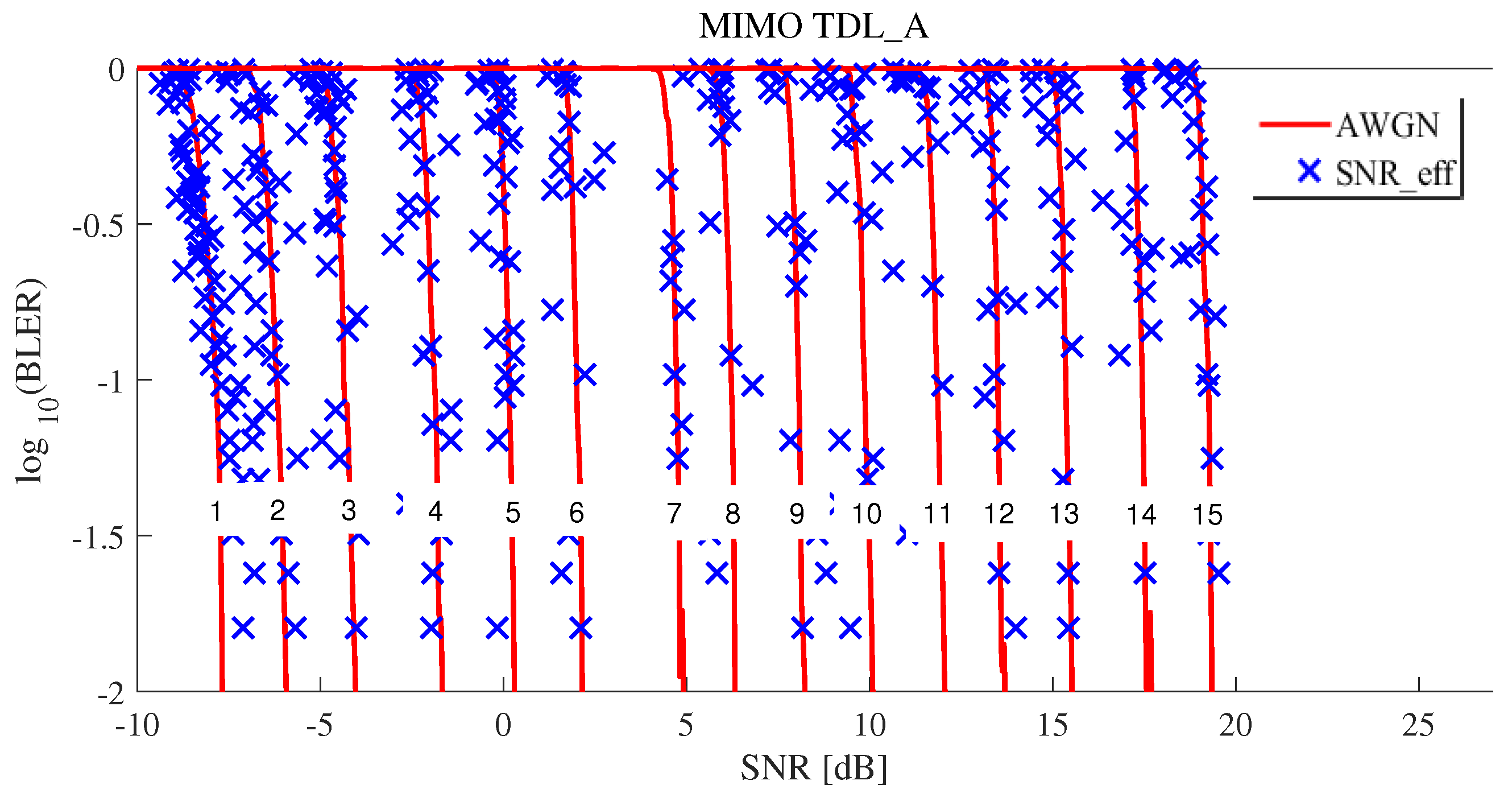
Figure 9 and Figure 10 show the results of effective SNR mapping by the proposed ML-based EESM method in the case of 5G TDL-A 2 × 2 MIMO. MIMO cases were also similar to SISO cases from the analytical point of view. As shown in Figure 9, were more widespread compared to SISO case shown in Figure 9. Therefore, since the variance of was larger than that of SISO, MSE of MIMO was also larger than that of SISO. Figure 10 shows how well is the effective SNR mapped to the AWGN for all CQIs under MIMO. Compared to SISO results, there were a few blue that were slightly off the AWGN line.
6. Conclusions
We proposed a novel link-to-system (L2S) mapping method based on machine learning (ML) for 5G new radio (NR) simulators, which reduces the computational complexity as well as improves the prediction accuracy of block error rates (BLERs) prediction. The performance of the proposed ML-based L2S mapping technique was validated by utilizing link-level simulator (LLS) of the 5G K-simulator. In particular, we adopted the optimizers such Adagrad and RMSProp for obtaining parameters for effective exponential signal-to-noise ratio mapping (EESM).
As a further study, we will investigate the ML-based decision process for the system-level simulator (SLS) to determine whether a received frame is successfully decoded without the L2S mapping procedure.
Author Contributions
E.C. performed conceptualization, methodology, and formal analysis; J.Y. performed computer simulations; B.C.J. created the basic idea and designed the experiments; E.C., J.Y. and B.C.J. wrote the paper.
Acknowledgments
This work was supported in part by the Basic Science Research Program through the NRF funded by the Ministry of Science and ICT under Grant NRF-2016R1A2B4014834, in part by “The Cross-Ministry Giga KOREA Project” grant from the Ministry of Science, ICT and Future Planning, Korea, [GK 18S0400, Research and Development of Open 5G Reference Model], and in part by the MSIT (Ministry of Science and ICT), Korea, under the ITRC (Information Technology Research Center) support program (IITP-2019-2017-0-01635) supervised by the IITP (Institute for Information & communications Technology Promotion).
Conflicts of Interest
The authors declare no conflict of interest. The founding sponsors had no role in the design of the study; in the collection, analyses, or interpretation of data; in the writing of the manuscript, and in the decision to publish the results.
References
- Chih-Lin, I.; Han, S.; Xu, Z.; Wang, S.; Sun, Q.; Chen, Y. New paradigm of 5G wireless internet. IEEE J. Sel. Areas Commun. 2016, 34, 474–482. [Google Scholar]
- ITU-R, Framework and Overall Objectives of the Future Development of IMT for 2020 and Beyond. Recommendations: M.2083. 2015. Available online: https://www.itu.int/rec/R-REC-M.2083-0-201509-I/en (accessed on 1 March 2019).
- Ding, Z.; Liu, Y.; Choi, J.; Sun, Q.; Elkashlan, M.; Poor, H.V. Application of non-orthogonal multiple access in LTE and 5G networks. IEEE Commun. Mag. 2017, 55, 185–191. [Google Scholar]
- Andrews, J.G. What will 5G be? IEEE J. Sel. Areas Commun. 2014, 32, 1065–1082. [Google Scholar] [CrossRef]
- Olmos, J.; Ruiz, S.; Gareia-Lozano, M.; Martin-Sacristan, D. Link Abstraction Models Based on Mutual Information for LTE Downlink; COST 2100 TD(10) 11052; iTEAM Research Institute: Aalborg, Denmark, 2010. [Google Scholar]
- Tuomaala, E.; Wang, H. Effective SINR approach of link to system mapping in OFDM/multi-carrier mobile network. In Proceedings of the IEEE the Second International Conference on Mobile Technology, Applications and Systems, Cape Town, South Africa, 15–17 November 2005; pp. 140–144. [Google Scholar]
- IEEE C802.16m-07097. Link Performance Abstraction Based on Mean Mutual Information Per Bit (MMIB) of the LLR Channel; IEEE 802.16 Broadband Wireless Access Working Group. 2007. Available online: http://www.wirelessman.org/tgm/contrib/C80216m-07_097.pdf (accessed on 1 March 2019).
- Hcine, M.B.; Bouallegue, R. Analysis of uplink effective SINR in LTE networks. In Proceedings of the 2015 International Wireless Communications and Mobile Computing Conference (IWCMC), Dubrovnik, Croatia, 24–28 August 2015. [Google Scholar]
- Hanzaz, Z.; Schotten, H.D. Impact of L2S interface on system level evaluation for LTE system. In Proceedings of the 2013 IEEE 11th Malaysia International Conference on Communications (MICC), Kuala Lumpur, Malaysia, 26–28 November 2013. [Google Scholar]
- Daniels, R.; Heath, R.W., Jr. Online adaptive modulation and coding with support vector machines. In Proceedings of the IEEE European Wireless Conference, Lucca, Italy, 12–15 April 2010; pp. 718–724. [Google Scholar]
- Mesa, A.C.; Aguayo-Torres, M.C.; Martin-Vega, F.J.; Gómez, G.; Blanquez-Casado, F.; Delgado-Luque, I.; Entrambasaguas, J. Link abstraction models for multicarrier systems: A logistic regression approach. Int. J. Commun. Syst. 2018, 31, e3436. [Google Scholar]
- Chu, E.; Jang, H.J.; Jung, B.C. Machine learning based link-to-system mapping for system-level simulation of cellular networks. In Proceedings of the 2018 Tenth International Conference on Ubiquitous and Future Networks, Prague, Czech Republic, 3–6 July 2018; pp. 503–506. [Google Scholar]
- Kim, Y.; Bae, J.; Lim, J.; Park, E.; Baek, J.; Han, S.I.; Han, Y. 5G K-Simulator: 5G System Simulator for Performance Evaluation. In Proceedings of the 2018 IEEE International Symposium on Dynamic Spectrum Access Networks (DySPAN), Seoul, Korea, 22–25 October 2018. [Google Scholar]
- Homepage of 5G K-Simulator. Available online: http://5gopenplatform.org/main/index.php (accessed on 1 March 2019).
- Berrou, C.; Glavieux, A.; Thitimajshima, P. Near Shannon limit error-correcting coding and decoding: Turbo codes. In Proceedings of the ICC ’93—IEEE International Conference on Communications, Geneva, Switzerland, 23–26 May 1993. [Google Scholar]
- MacKay, D.J.C.; Neal, R.M. Near Shannon limit performance of low density parity check codes. Electron. Lett. 1996, 32, 1645–1646. [Google Scholar] [CrossRef]
- Arikan, E. Channel polarization: A method for constructing capacity achieving codes for symmetric binary-input memoryless channels. IEEE Trans. Inf. Theory 2008, 55, 3051–3073. [Google Scholar] [CrossRef]
- 3rd Generation Partnership Project; Technical Specification Group Radio access Network (3GPP), TR 38.900 (V15.0.0), Study on Channel Model for Frequency Spectrum Above 6 GHz. July 2018. Available online: https://portal.3gpp.org/desktopmodules/Specifications/SpecificationDetails.aspx?specificationId=2991 (accessed on 1 March 2019).
- 3rd Generation Partnership Project; Technical Specification Group Radio access Network (3GPP), TR 38.901 (V15.0.0), Study on Channel Model for Frequency From 0.5 To 100 GHz. June 2018. Available online: https://portal.3gpp.org/desktopmodules/Specifications/SpecificationDetails.aspx?specificationId=3173 (accessed on 1 March 2019).
- 3rd Generation Partnership Project; Technical Specification Group Radio access Network (3GPP), TR 38.802 (V14.0.0), Study on New Radio Access Technology Physical Layer Aspects. March 2017. Available online: https://portal.3gpp.org/desktopmodules/Specifications/SpecificationDetails.aspx?specificationId=3066 (accessed on 1 March 2019).
- 3rd Generation Partnership Project; Technical Specification Group Radio access Network (3GPP), TS 38.211 (V15.3.0), Evolved Universal Terrestrial Radio Access (E-UTRA): Physical channels and modulation. 2018. Available online: https://portal.3gpp.org/desktopmodules/Specifications/SpecificationDetails.aspx?specificationId=3213 (accessed on 1 March 2018).
- Ruder, S. An overview of gradient descent optimization algorithms. arXiv, 2016; arXiv:1609.04747. [Google Scholar]
- Goodfellow, I.; Bengio, Y.; Courville, A.; Bach, F. Deep Learning (Adaptive Computation and Machine Learning Series); MIT Press: Cambridge, MA, USA, 2006. [Google Scholar]
Figure 1.
Downlink resource grid [21].
Figure 1.
Downlink resource grid [21].

Figure 2.
Schematic of 5G NR L2S mapping.
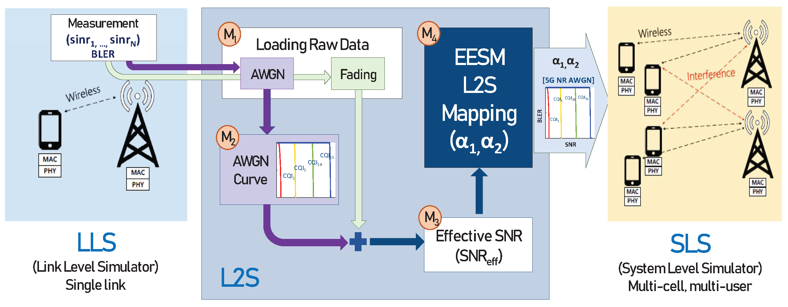
Figure 3.
Deep neural network.

Figure 4.
SNR vs. BLER for CQI 1 under 4G AWGN channel [12].
Figure 4.
SNR vs. BLER for CQI 1 under 4G AWGN channel [12].

Figure 5.
The BLER comparison between 4G AWGN and 5G AWGN.

Figure 6.
SNR threshold for all CQIs under 5G AWGN.
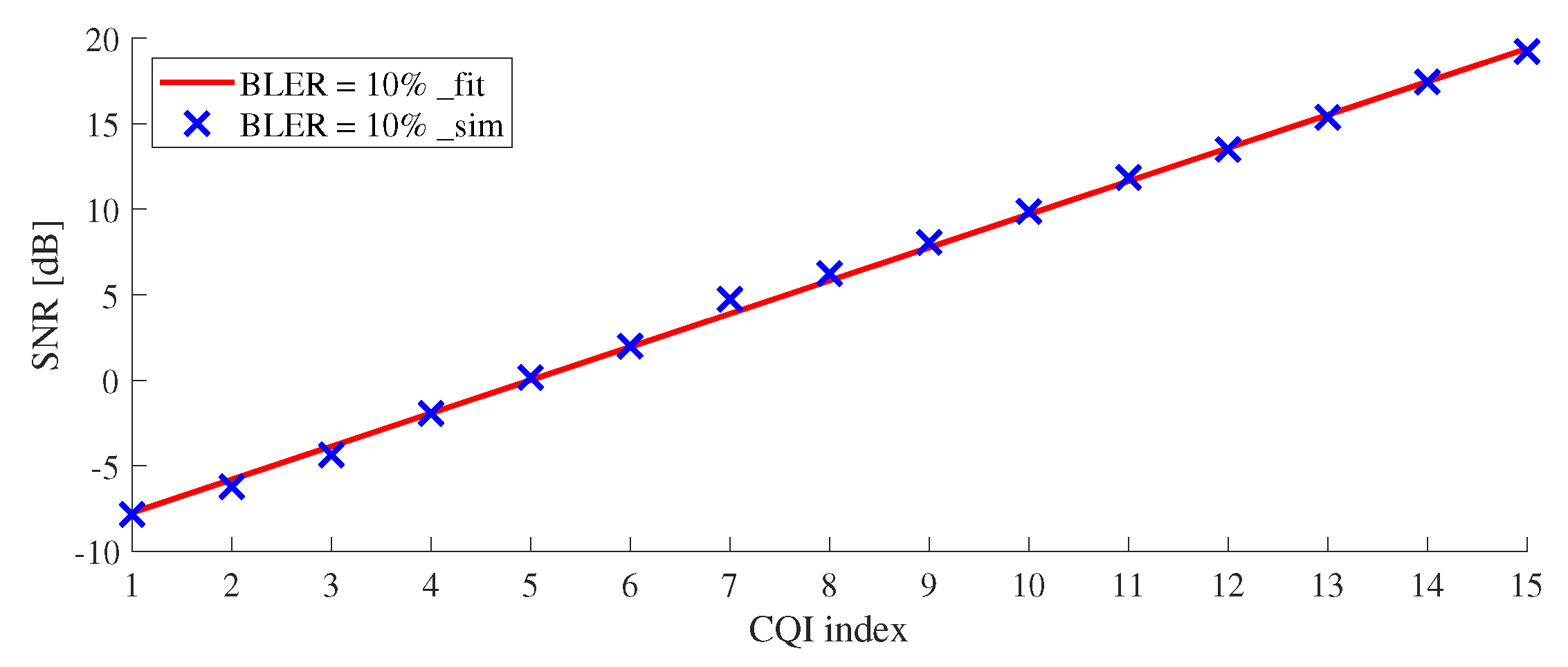
Figure 7.
Effective SNR mapping results of the proposed ML-based EESM method under 5G CDL-A SISO (for CQI1, CQI5, CQI10, and CQI15).
Figure 7.
Effective SNR mapping results of the proposed ML-based EESM method under 5G CDL-A SISO (for CQI1, CQI5, CQI10, and CQI15).
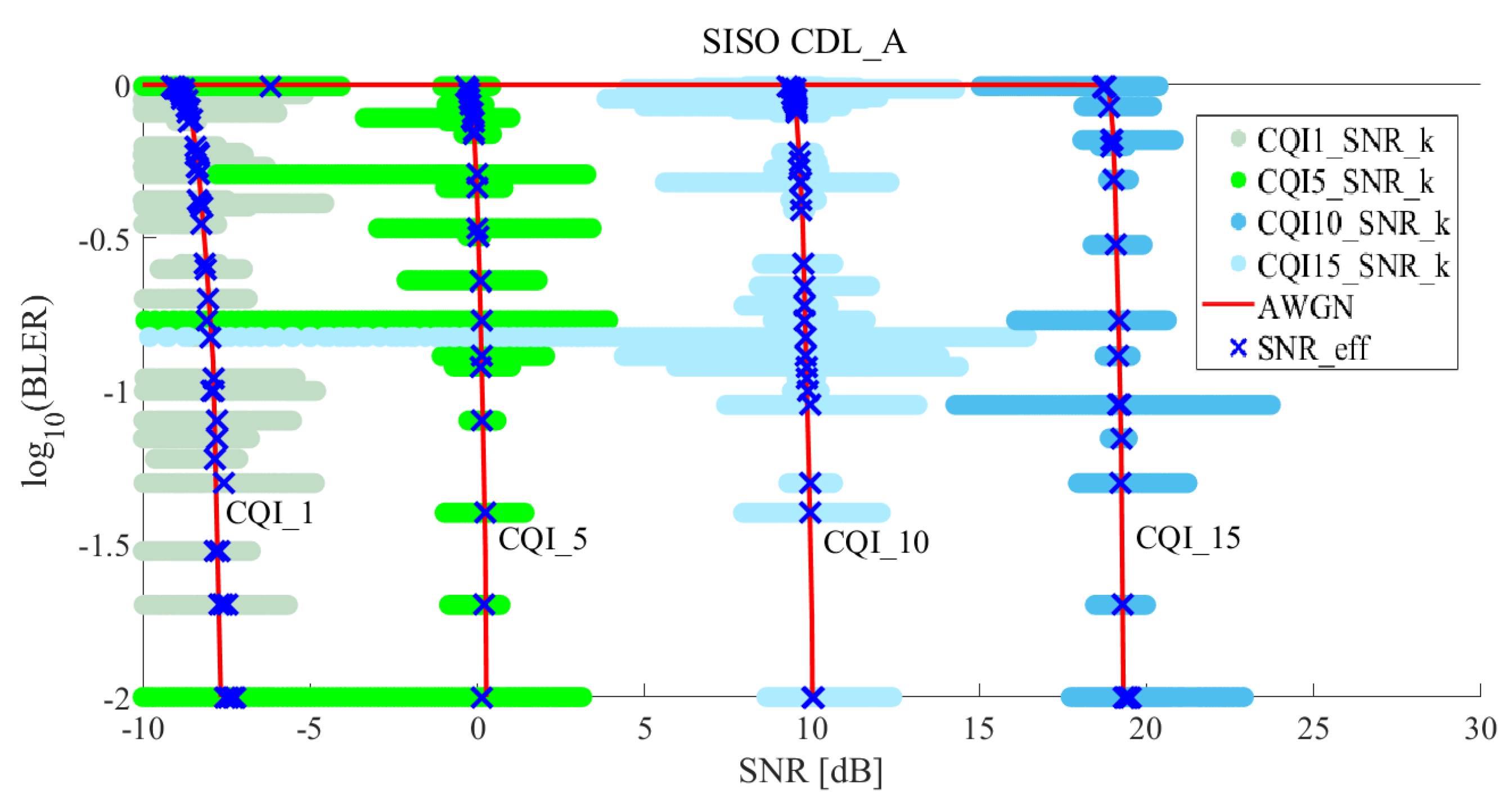
Figure 8.
Effective SNR mapping results of the proposed ML-based EESM method under 5G CDL-A SISO for all CQIs.
Figure 8.
Effective SNR mapping results of the proposed ML-based EESM method under 5G CDL-A SISO for all CQIs.
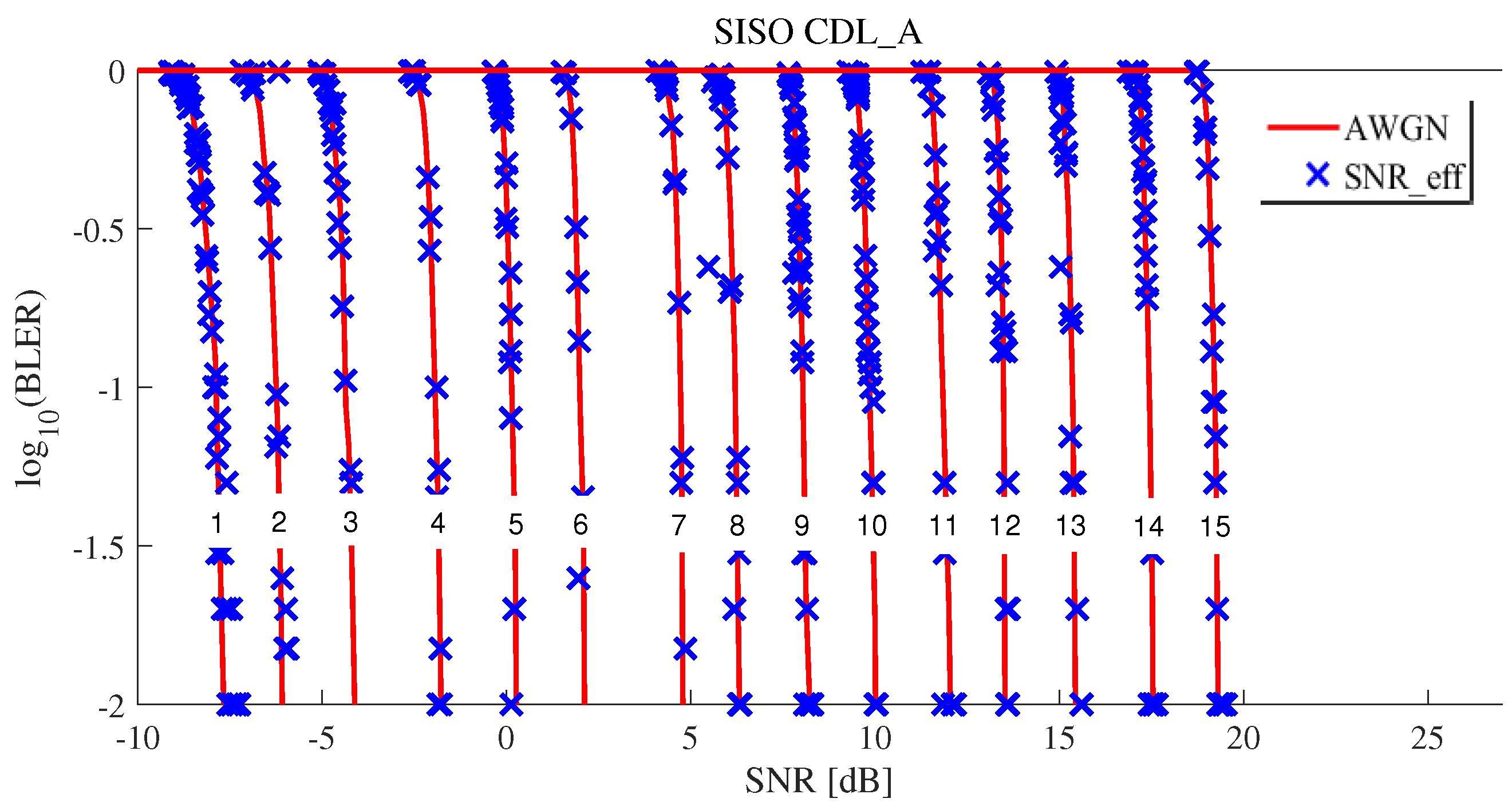
Figure 9.
Effective SNR mapping results of the proposed ML-based EESM method under 5G TDL-A 2 × 2 MIMO (for CQI1, CQI5, CQI10, and CQI15).
Figure 9.
Effective SNR mapping results of the proposed ML-based EESM method under 5G TDL-A 2 × 2 MIMO (for CQI1, CQI5, CQI10, and CQI15).
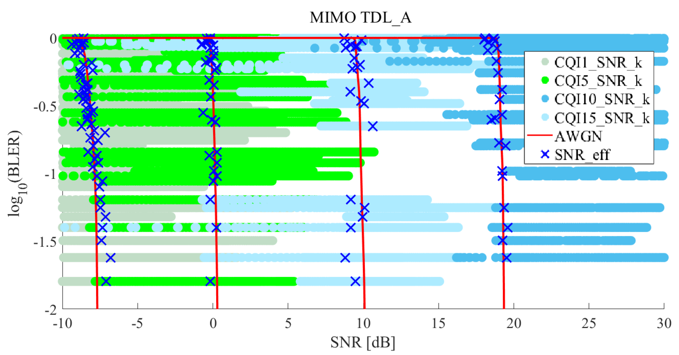
Figure 10.
Effective SNR mapping results of the proposed ML-based EESM method under 5G TDL-A 2 × 2 MIMO for all CQIs.
Figure 10.
Effective SNR mapping results of the proposed ML-based EESM method under 5G TDL-A 2 × 2 MIMO for all CQIs.


Table 1.
Abbreviations.
| Abbreviation: Full Name | Abbreviation: Full Name |
|---|---|
| AWGN: additive white Gaussian noise | BLER: block error rate |
| CQI: channel quality indication | CDL: clustered delay line |
| DNN: deep neural network | EESM: exponential effective SNR mapping |
| eNB: evolved Node-B | LDPC: Low-density parity-check |
| LTE-A: long term evolution-advanced | LLS: link-level simulator |
| L2S: link-to-system | MIMO: multiple input multiple output |
| ML: machine learning | MMSE: minimum mean square error |
| MSE: mean squared error | NS: network-level simulator |
| NR: new radio | RB: resource block |
| RE: resource element | SINR: signal-to-interference plus noise ratio |
| SISO: single input single output | SLS: system-level simulator |
| SNR: signal-to-noise ratio | TB: transport block |
| TDL: tapped delay line | UE: user equipment |
Table 2.
System configuration/setup.
| Parameters | Values |
|---|---|
| Waveform | OFDM |
| Carrier frequency | 2.8 GHz |
| Bandwidth | 5 MHz |
| Sub-carrier spacing | kHz |
| Channel Estimation | Perfect, MMSE |
| The number of allocated RBs to a UE | 25 RBs |
| The number of sub-carriers per RB | 12 sub-carriers |
| The number of symbols per slot | 7 symbols |
| The number of slots per sub-frame | 2 slots |
| Channel Coding | Turbo-Code (4G), LDPC (5G) |
| Channel Model | AWGN, CDL-A (SISO), TDL-A ( MIMO) |
Table 3.
Channel Quality Indication (CQI) table for turbo-code and LDPC.
| LDPC | Turbo Code | ||||||||
|---|---|---|---|---|---|---|---|---|---|
| CQI | Mod. | ||||||||
| [Bits] | [Bits] | × | [Bits] | [Bits] | × | ||||
| 1 | QPSK | 584 | 8000 | 0.0762 | 0.1523 | 608 | 7800 | 0.0779 | 0.1559 |
| 2 | QPSK | 912 | 8000 | 0.1172 | 0.2344 | 928 | 7800 | 0.1190 | 0.2379 |
| 3 | QPSK | 1480 | 8000 | 0.1885 | 0.3770 | 1480 | 7800 | 0.1897 | 0.3795 |
| 4 | QPSK | 2384 | 8000 | 0.3008 | 0.6016 | 2408 | 7800 | 0.3087 | 0.6174 |
| 5 | QPSK | 3480 | 8000 | 0.4385 | 0.8770 | 3496 | 7800 | 0.4482 | 0.8964 |
| 6 | QPSK | 4680 | 8000 | 0.5879 | 1.1758 | 4608 | 7800 | 0.5908 | 1.1815 |
| 7 | 16QAM | 5880 | 16,000 | 0.3691 | 1.4766 | 5760 | 15,600 | 0.3692 | 1.4769 |
| 8 | 16QAM | 7632 | 16,000 | 0.4785 | 1.9141 | 7424 | 15,600 | 0.4759 | 1.9036 |
| 9 | 16QAM | 9600 | 16,000 | 0.6016 | 2.4063 | 9480 | 15,600 | 0.6077 | 2.4308 |
| 10 | 64QAM | 10,896 | 24,000 | 0.4551 | 2.7305 | 10,760 | 23,400 | 0.4598 | 2.7590 |
| 11 | 64QAM | 13,264 | 24,000 | 0.5537 | 3.3223 | 13,064 | 23,400 | 0.5583 | 3.3497 |
| 12 | 64QAM | 15,584 | 24,000 | 0.6504 | 3.9023 | 15,112 | 23,400 | 0.6458 | 3.8749 |
| 13 | 64QAM | 18,072 | 24,000 | 0.7539 | 4.5234 | 17,424 | 23,400 | 0.7446 | 4.4677 |
| 14 | 64QAM | 20,440 | 24,000 | 0.8525 | 5.1152 | 19,968 | 23,400 | 0.8533 | 5.1200 |
| 15 | 64QAM | 22,192 | 24,000 | 0.9258 | 5.5547 | 21,504 | 23,400 | 0.9190 | 5.5138 |
Table 4.
The comparison of MSE under 4G AWGN channel [12].
Table 4.
The comparison of MSE under 4G AWGN channel [12].
| CQI Index | CQI 1 | CQI 2 | CQI 3 | CQI 4 | CQI 5 | CQI 6 | CQI 7 | CQI 8 |
|---|---|---|---|---|---|---|---|---|
| FIT | 0.033 | 0.027 | 0.033 | 0.038 | 0.017 | 0.032 | 0.017 | 0.012 |
| DNN | 0.018 | 0.014 | 0.016 | 0.013 | 0.014 | 0.011 | 0.015 | 0.016 |
| CQI Index | CQI 9 | CQI 10 | CQI 11 | CQI 12 | CQI 13 | CQI 14 | CQI 15 | - |
| FIT | 0.019 | 0.021 | 0.011 | 0.025 | 0.013 | 0.015 | 0.030 | - |
| DNN | 0.011 | 0.008 | 0.013 | 0.013 | 0.010 | 0.013 | 0.010 | - |
Table 5.
The values of SNR Threshold satisfying 10% BLER.
| CQI Index | CQI 1 | CQI 2 | CQI 3 | CQI 4 | CQI 5 | CQI 6 | CQI 7 | CQI 8 |
|---|---|---|---|---|---|---|---|---|
| SNR Threshold [dB] | −7.8474 | −6.2369 | −4.3591 | −1.9319 | 0.1509 | 1.9976 | 4.7278 | 6.2231 |
| CQI Index | CQI 9 | CQI 10 | CQI 11 | CQI 12 | CQI 13 | CQI 14 | CQI 15 | - |
| SNR Threshold [dB] | 8.0591 | 9.8585 | 11.8432 | 13.4893 | 15.3598 | 17.4435 | 19.2155 | - |
Table 6.
Optimal parameters in 5G CDL-A SISO.
| CQI | AdaGrad | RMSProp | |||||
|---|---|---|---|---|---|---|---|
| MSE | MSE | ||||||
| 1 | 3.294 | 3.230 | 0.150 | 2.752 | 2.698 | 0.149 | |
| 2 | 1.874 | 1.880 | 0.357 | 2.163 | 2.170 | 0.364 | |
| 3 | 1.607 | 1.594 | 0.065 | 2.002 | 1.988 | 0.061 | |
| 4 | 1.184 | 1.175 | 0.159 | 1.162 | 1.154 | 0.156 | |
| 5 | 1.286 | 1.283 | 0.140 | 1.552 | 1.546 | 0.206 | |
| 6 | 1.359 | 1.359 | 0.055 | 1.360 | 0.360 | 0.056 | |
| 7 | 3.642 | 3.628 | 0.170 | 3.643 | 3.629 | 0.170 | |
| 8 | 3.256 | 3.228 | 0.171 | 3.937 | 3.911 | 0.155 | |
| 9 | 5.563 | 5.543 | 0.110 | 5.636 | 5.616 | 0.110 | |
| 10 | 16.259 | 16.204 | 0.075 | 16.262 | 16.208 | 0.075 | |
| 11 | 13.685 | 13.604 | 0.329 | 13.382 | 13.301 | 0.268 | |
| 12 | 17.988 | 18.079 | 0.778 | 17.547 | 17.632 | 0.724 | |
| 13 | 23.971 | 23.970 | 0.555 | 24.112 | 24.111 | 0.558 | |
| 14 | 29.306 | 29.205 | 0.210 | 29.306 | 29.204 | 0.210 | |
| 15 | 33.590 | 33.833 | 0.533 | 28.733 | 28.739 | 0.823 | |
Table 7.
Optimal parameters in 5G TDL-A 2 × 2 MIMO.
| CQI | AdaGrad | RMSProp | |||||
|---|---|---|---|---|---|---|---|
| MSE | MSE | ||||||
| 1 | 0.088 | 0.126 | 1.581 | 0.079 | 0.106 | 1.465 | |
| 2 | 0.114 | 0.154 | 0.834 | 0.114 | 0.152 | 0.969 | |
| 3 | 0.200 | 0.252 | 0.730 | 0.208 | 0.260 | 1.070 | |
| 4 | 0.280 | 0.306 | 0.867 | 0.301 | 0.339 | 0.976 | |
| 5 | 0.511 | 0.525 | 0.859 | 0.513 | 0.528 | 0.865 | |
| 6 | 0.718 | 0.729 | 2.072 | 0.718 | 0.729 | 2.070 | |
| 7 | 2.664 | 3.554 | 1.526 | 2.664 | 3.553 | 1.528 | |
| 8 | 2.465 | 2.665 | 1.538 | 2.465 | 2.664 | 1.525 | |
| 9 | 3.200 | 4.695 | 1.782 | 3.203 | 4.700 | 1.784 | |
| 10 | 6.532 | 8.174 | 1.824 | 6.338 | 7.900 | 1.777 | |
| 11 | 6.588 | 8.619 | 0.703 | 5.969 | 7.634 | 0.688 | |
| 12 | 9.985 | 11.538 | 1.125 | 10.021 | 11.661 | 1.135 | |
| 13 | 11.190 | 14.225 | 1.393 | 11.19 | 14.224 | 1.399 | |
| 14 | 15.933 | 19.071 | 0.973 | 19.562 | 23.828 | 2.784 | |
| 15 | 20.410 | 38.530 | 1.399 | 19.062 | 34.963 | 1.099 | |
© 2019 by the authors. Licensee MDPI, Basel, Switzerland. This article is an open access article distributed under the terms and conditions of the Creative Commons Attribution (CC BY) license (http://creativecommons.org/licenses/by/4.0/).
Share and Cite
MDPI and ACS Style
Chu, E.; Yoon, J.; Jung, B.C. A Novel Link-to-System Mapping Technique Based on Machine Learning for 5G/IoT Wireless Networks. Sensors 2019, 19, 1196. https://doi.org/10.3390/s19051196
AMA Style
Chu E, Yoon J, Jung BC. A Novel Link-to-System Mapping Technique Based on Machine Learning for 5G/IoT Wireless Networks. Sensors. 2019; 19(5):1196. https://doi.org/10.3390/s19051196
Chicago/Turabian StyleChu, Eunmi, Janghyuk Yoon, and Bang Chul Jung. 2019. "A Novel Link-to-System Mapping Technique Based on Machine Learning for 5G/IoT Wireless Networks" Sensors 19, no. 5: 1196. https://doi.org/10.3390/s19051196
Note that from the first issue of 2016, this journal uses article numbers instead of page numbers. See further details here.