Estimating Spatial and Temporal Trends in Environmental Indices Based on Satellite Data: A Two-Step Approach


Abstract
1. Introduction
2. Data Description
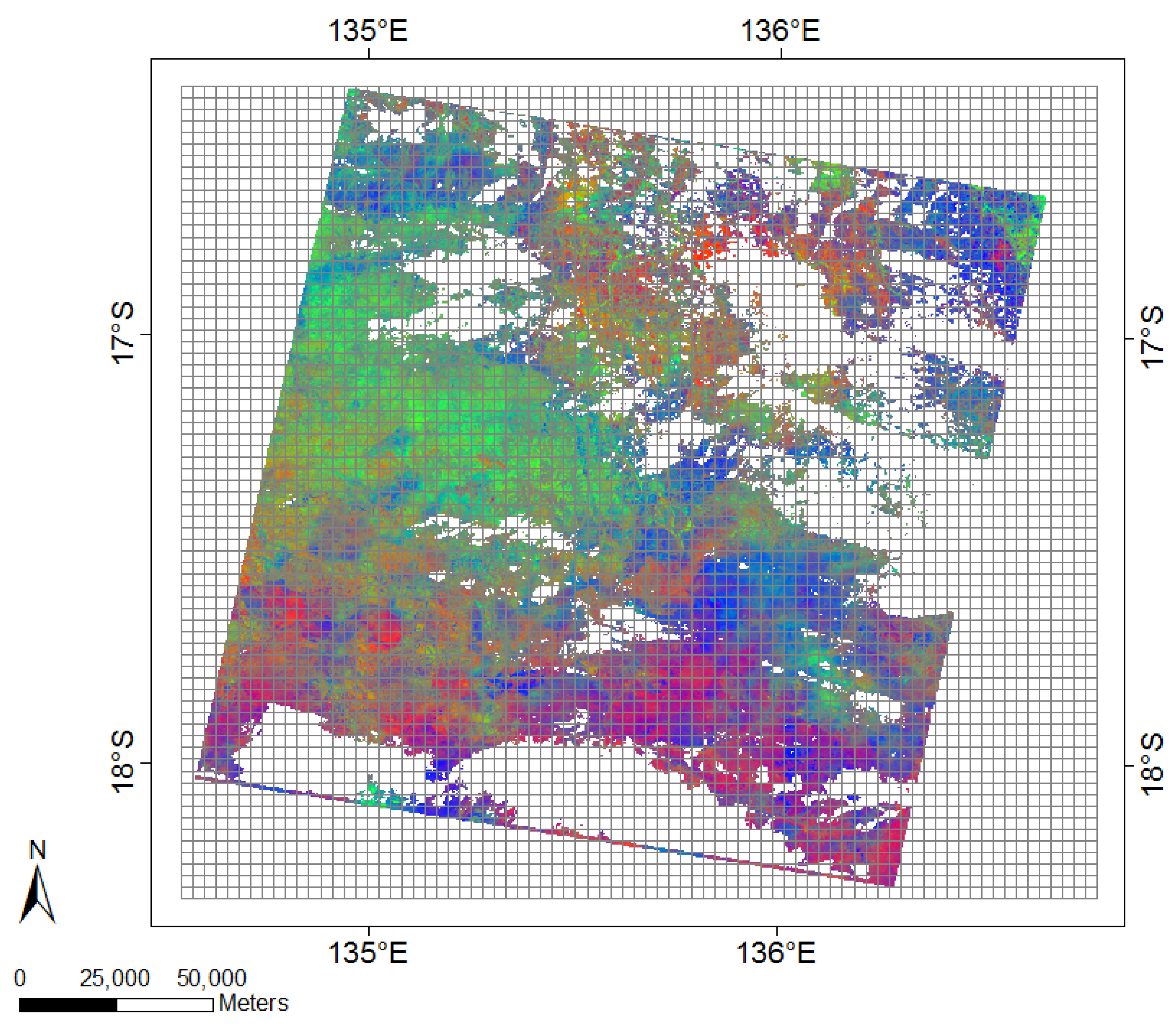
2.1. Case Study
2.2. Fractional Cover Data
2.3. Data Pre-Processing
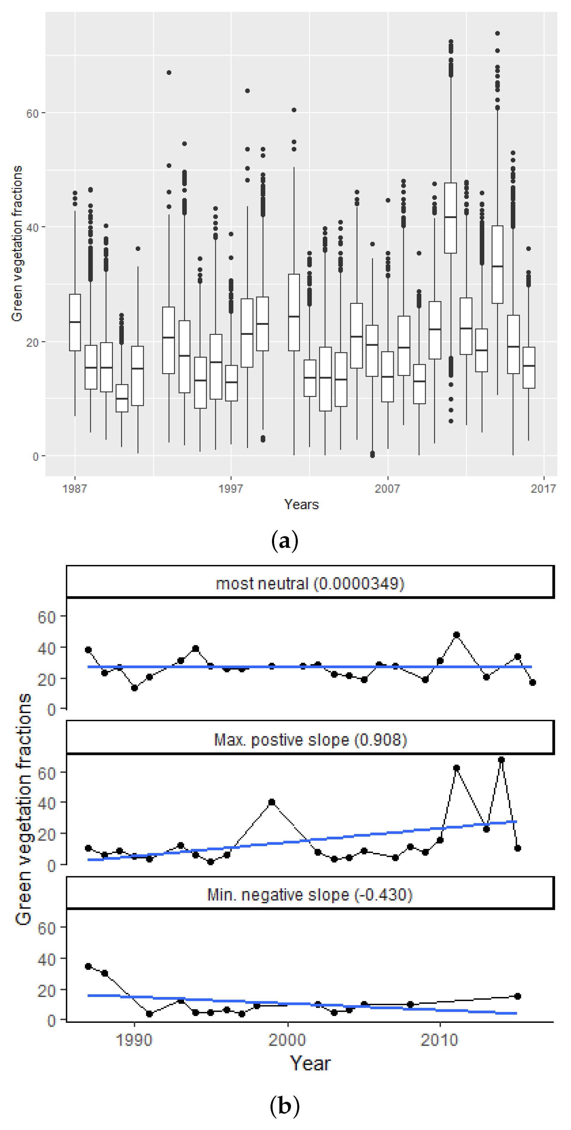
2.4. Data Exploration
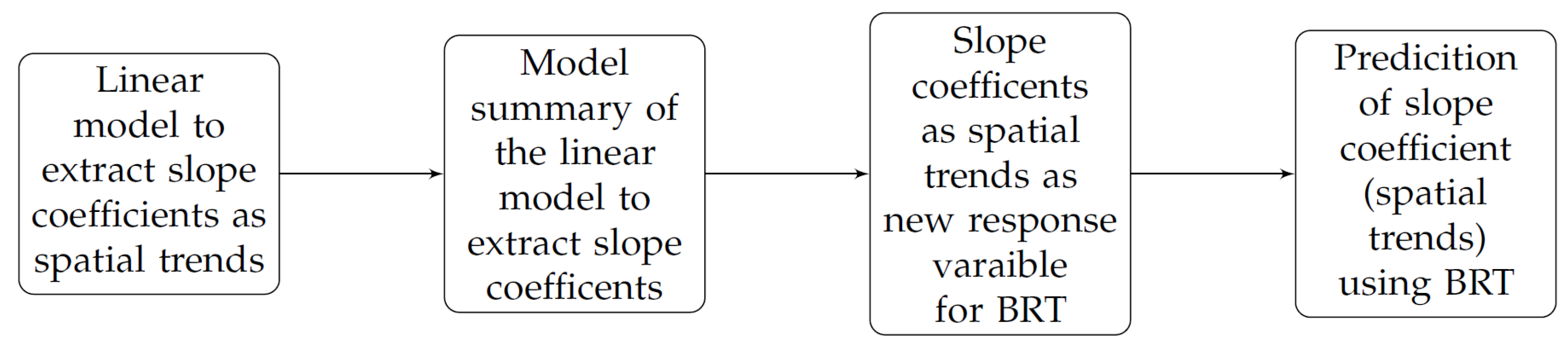
3. Methods
3.1. Linear Model
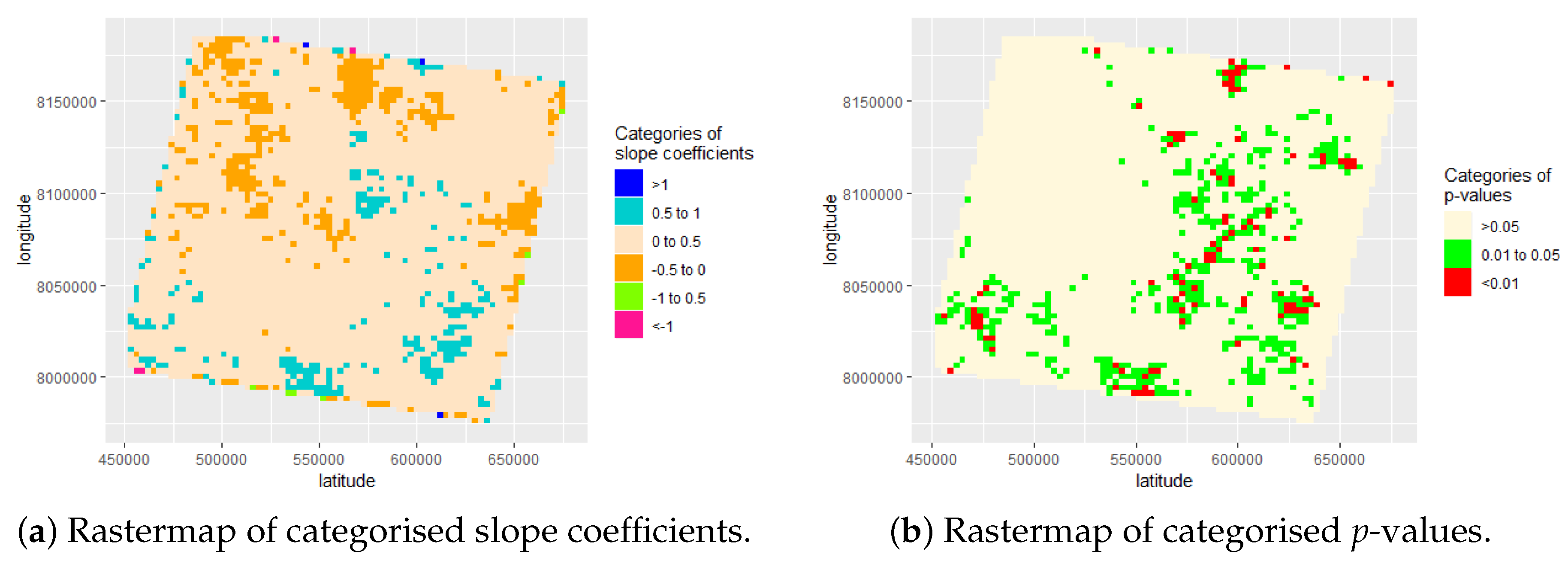
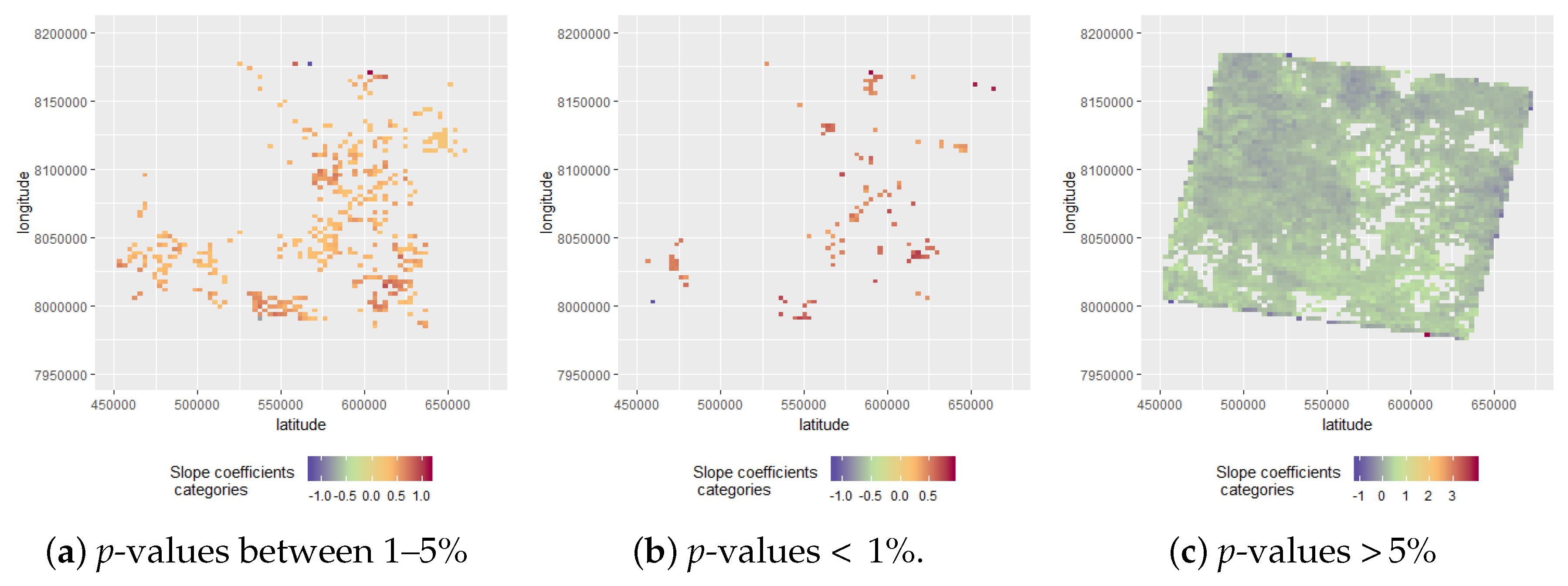
3.1.1. Extraction of Slope Coefficients
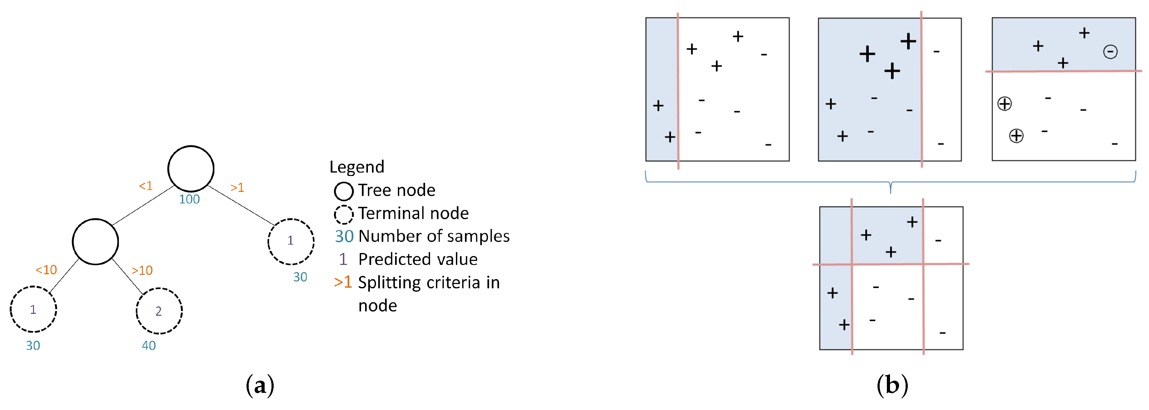
3.2. Boosted Regression Tree
Hyperparameter Tuning and Goodness of Fit Evaluation
4. Results
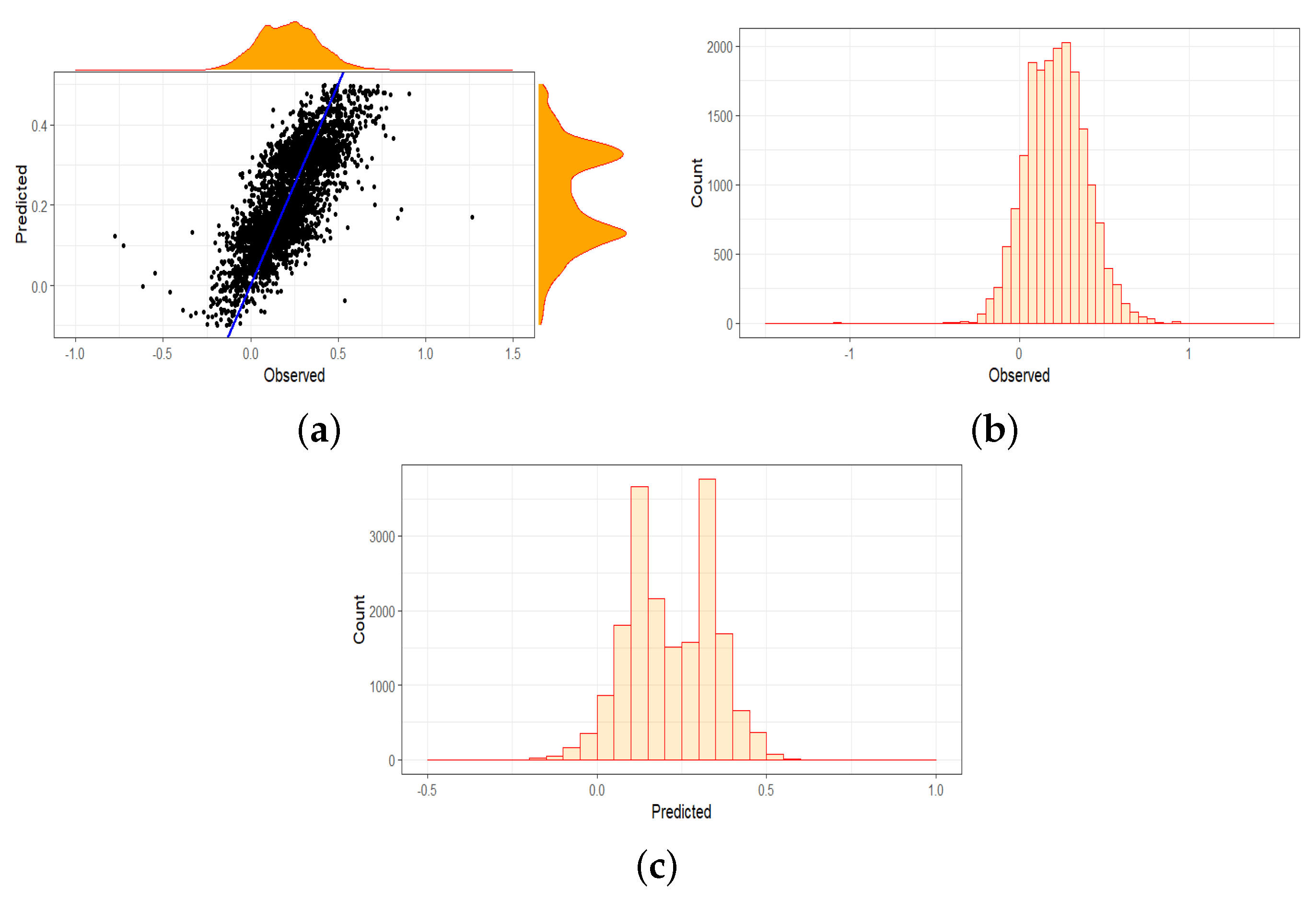
4.1. BRT Predictions
4.1.1. Overall Results of the Entire Data Set
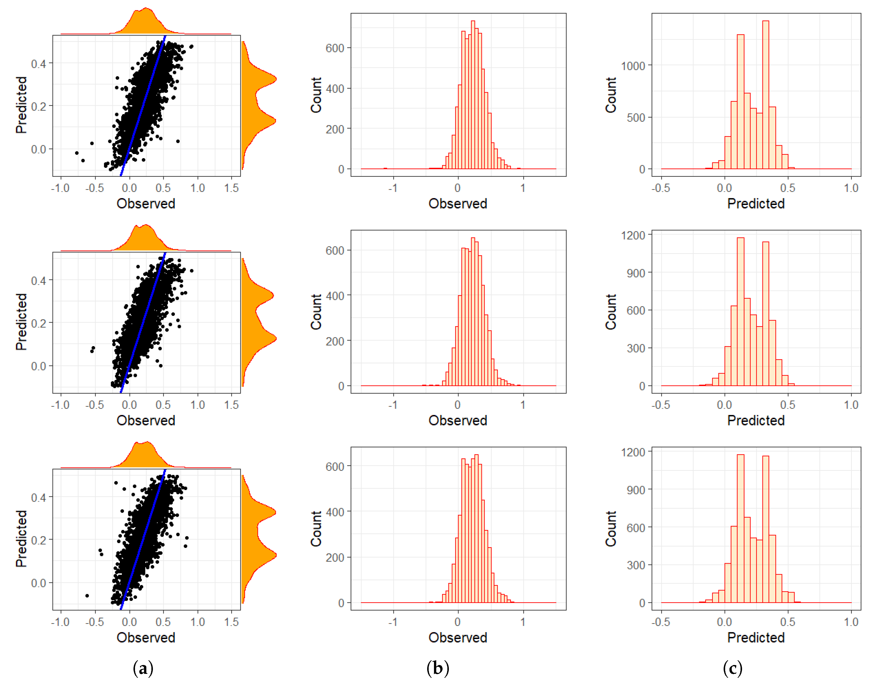
4.1.2. Decadal Analyses
4.1.3. Segmented Areas
4.2. Relative Influence
5. Discussion
6. Conclusions
Author Contributions
Funding
Acknowledgments
Conflicts of Interest
References
- Wulder, M.A.; Masek, J.G.; Cohen, W.B.; Loveland, T.R.; Woodcock, C.E. Opening the archive: How free data has enabled the science and monitoring promise of Landsat. Remote Sens. Environ. 2012, 2–10. [Google Scholar] [CrossRef]
- Walsh, S.J.; Crawford, T.W.; Welsh, W.F.; Crews-Meyer, K.A. A multiscale analysis of LULC and NDVI variation in Nang Rong district, northeast Thailand. Agric. Ecosyst. Environ. 2001, 85, 47–64. [Google Scholar] [CrossRef]
- Gallo, K.P.; Easterling, D.R.; Peterson, T.C. The Influence of Land Use/Land Cover on Climatological Values of the Diurnal Temperature Range. J. Clim. 1996, 9, 2941–2944. [Google Scholar] [CrossRef]
- Datt, B. A New Reflectance Index for Remote Sensing of Chlorophyll Content in Higher Plants: Tests using Eucalyptus Leaves. J. Plant Physiol. 1999, 154, 30–36. [Google Scholar] [CrossRef]
- Zhang, H.; Li, Q.Z.; Lei, F.; Du, X.; Wei, J.D. Research on rice acreage estimation in fragmented area based on decomposition of mixed pixels. Remote Sens. Spat. Inf. Sci. 2015, 40, 133. [Google Scholar] [CrossRef]
- Guerschman, J.P.; Scarth, P.F.; McVicar, T.R.; Renzullo, L.J.; Malthus, T.J.; Stewart, J.B.; Rickards, J.E.; Trevithick, R. Assessing the effects of site heterogeneity and soil properties when unmixing photosynthetic vegetation, non-photosynthetic vegetation and bare soil fractions from Landsat and MODIS data. Remote Sens. Environ. 2015, 161, 12–26. [Google Scholar] [CrossRef]
- Adams, J.B.; Sabol, D.E.; Kapos, V.; Filho, R.A.; Roberts, D.A.; Smith, M.O.; Gillespie, A.R. Classification of multispectral images based on fractions of endmembers: Application to land-cover change in the Brazilian Amazon. Remote Sens. Environ. 1995, 52, 137–154. [Google Scholar] [CrossRef]
- Roberts, D.A.; Smith, M.A.J. Green vegetation, nonphotosynthetic vegetation, and soils in AVIRIS data. Remote Sens. Environ. 1993, 44, 255–269. [Google Scholar] [CrossRef]
- Zachary, T.; Dar, R.; Sander, V.; Angeles, C.; Carlos, R.; Susan, U. Evaluating Endmember and Band Selection Techniques for Multiple Endmember Spectral Mixture Analysis using Post-Fire Imaging Spectroscopy. Remote Sens. 2018, 10, 389. [Google Scholar] [CrossRef]
- Scarth, P.F.; Röder, A.; Schmidt, M. Tracking Grazing pressure and climate interaction—The Role of Landsat Fractional Cover in time series analysis. In Proceedings of the 15th Australasian Remote Sensing and Photogrammetry Conference, Alice Springs, Australia, 13–17 September 2010; p. 13. [Google Scholar] [CrossRef]
- Scanlon, T.M.; Albertson, J.D.; Caylor, K.K.; Williams, C.A. Determining land surface fractional cover from NDVI and rainfall time series for a savanna ecosystem. Remote Sens. Environ. 2002, 82, 376–388. [Google Scholar] [CrossRef]
- Colin, B.; Schmidt, M.; Clifford, S.; Woodley, A.; Mengersen, K. Influence of Spatial Aggregation on Prediction Accuracy of Green Vegetation Using Boosted Regression Trees. Remote Sens. 2018, 10, 1260. [Google Scholar] [CrossRef]
- McNab, H.W.; Lloyd, T.F. Testing Ecoregions in Kentucky and Tennessee with Satellite Imagery and Forest Inventory Data: USDA Forest Service Proceedings—RMRS-P-56. 2009; Number 10; pp. 1–19. Available online: https://www.fs.usda.gov/treesearch/pubs/all/33366 (accessed on 14 January 2019).
- Paruelo, J.M.; Lauenroth, W.K. Relative Abundance of Plant Functional Types in Grasslands and Shrublands of North America. Ecol. Appl. 1996, 6, 1212–1224. [Google Scholar] [CrossRef]
- Živadinović, I.; Ilijević, K.; Gržetić, I.; Popović, A. Long-term changes in the eco-chemical status of the Danube River in the region of Serbia. J. Serb. Chem. Soc. 2010, 75, 1125–1148. [Google Scholar] [CrossRef]
- Waller, L.A.; Gotway, C.A. Applied Spatial Statistics for Public Health Data; Wiley Series in Probability and Statistics: New York, NY, USA, 2004. [Google Scholar]
- Gaüzère, P.; Jiguet, F.; Devictor, V. Rapid adjustment of bird community compositions to local climatic variations and its functional consequences. Glob. Chang. Biol. 2015, 21, 3367–3378. [Google Scholar] [CrossRef] [PubMed]
- Zewdie, W.; Csaplovics, E.; Inostroza, L. Monitoring ecosystem dynamics in northwestern Ethiopia using NDVI and climate variables to assess long-term trends in dryland vegetation variability. Appl. Geogr. 2017, 79, 167–178. [Google Scholar] [CrossRef]
- Parisien, M.A.; Parks, S.A.; Krawchuk, M.A.; Flannigan, M.D.; Bowman, L.M.; Moritz, M.A. Scale-dependent controls on the area burned in the boreal forest of Canada, 1980–2005. Ecol. Appl. 2011, 21, 789–805. [Google Scholar] [CrossRef] [PubMed]
- Colin, B.; Clifford, S.; Wu, P.; Rathmanner, S.; Mengersen, K. Using Boosted Regression Trees and Remotely Sensed Data to Drive Decision-Making. Open J. Stat. 2017, 7, 859–875. [Google Scholar] [CrossRef]
- Bureau of Meteorology. Climate Classification of Australia. Available online: http://www.bom.gov.au/jsp/ncc/climateaverages/climate-classifications/index.jsp (accessed on 14 January 2019).
- Schmetz, J.; Pili, P.; Tjemkes, S.; Just, D.; Kerkmann, J.; Rota, S.; Ratier, A. An introduction to Meteosat second generation (MSG). Bull. Am. Meteorol. Soc. 2002, 83, 977–992. [Google Scholar] [CrossRef]
- Geiger, B.; Carrer, D.; Franchisteguy, L.; Roujean, J.L.; Meurey, C. Land surface albedo derived on a daily basis from Meteosat Second Generation observations. IEEE Trans. Geosci. Remote Sens. 2008, 46, 3841–3856. [Google Scholar] [CrossRef]
- Fensholt, R.; Sandholt, I.; Stisen, S.; Tucker, C. Analysing NDVI for the African continent using the geostationary meteosat second generation SEVIRI sensor. Remote Sens. Environ. 2006, 101, 212–229. [Google Scholar] [CrossRef]
- R Core Team. R: A Language and Environment for Statistical Computing; R Foundation for Statistical Computing: Vienna, Austria, 2013. [Google Scholar]
- R Development Core Team. 2008. Available online: https://cran.r-project.org/bin/windows/base/old/3.3.3/ (accessed on 14 January 2019).
- Elith, J.; Leathwick, J.R.; Hastie, T. A working guide to boosted regression trees. J. Anim. Ecol. 2008, 77, 802–813. [Google Scholar] [CrossRef] [PubMed]
- Matteson, A. Boosting the Accuracy of Your Machine Learning Models. 2013. Available online: https://www.datasciencecentral.com/profiles/blogs/boosting-the-accuracy-of-your-machine-learning-models (accessed on 14 January 2019).
- Hastie, T.J.; Tibshirani, R. Generalized additive models. Stat. Sci. 1986, 1, 297–318. [Google Scholar] [CrossRef]
- Moisen, G.G.; Freeman, E.A.; Blackard, J.A.; Frescino, T.S.; Zimmermann, N.E.; Edwards, T.C. Predicting tree species presence and basal area in Utah: A comparison of stochastic gradient boosting, generalized additive models, and tree-based methods. Ecol. Model. 2006, 199, 176–187. [Google Scholar] [CrossRef]
- Leathwick, J.R.; Elith, J.; Francis, M.P.; Hastie, T.; Taylor, P. Variation in demersal fish species richness in the oceans surrounding New Zealand: an analysis using boosted regression trees. Mar. Ecol.-Prog. Ser. 2006, 321, 267–281. [Google Scholar] [CrossRef]
- Kuhn, M. The caret Package. J. Stat. Softw. 2008, 5, 1–10. [Google Scholar]
- Ridgeway, G. Generalized Boosted Models: A Guide to the Gbm Package. Available online: https://www.semanticscholar.org/paper/Generalized-Boosted-Models-%3A-A-guide-to-the-gbm-Ridgeway/51eedf971c49610c8e006b0c6590315abd4645a9 (accessed on 14 January 2019).
- Liu, K.; Subbarayan, S.; Shoults, R.; Manry, M.; Kwan, C.; Lewis, F.; Naccarino, J. Comparison of very short-term load forecasting techniques. IEEE Trans. Power Syst. 1996, 11, 877–882. [Google Scholar] [CrossRef]
- Shi, J.; Lee, W.J.; Liu, Y.; Yang, Y.; Wang, P. Forecasting power output of photovoltaic systems based on weather classification and support vector machines. IEEE Trans. Ind. Appl. 2012, 48, 1064–1069. [Google Scholar] [CrossRef]
- Methaprayoon, K.; Yingvivatanapong, C.; Lee, W.J.; Liao, J.R. An integration of ANN wind power estimation into unit commitment considering the forecasting uncertainty. IEEE Trans. Ind. Appl. 2007, 43, 1441–1448. [Google Scholar] [CrossRef]


| Min. | 1st Qu. | Median | Mean | 3rd Qu. | Max. |
|---|---|---|---|---|---|
| 0.00 | 11.64 | 17.03 | 18.37 | 23.16 | 73.92 |
| Slope Coefficient Categories | Observations | Percentages % |
|---|---|---|
| slope coefficient > 1 | 14 | 0.02% |
| slope coefficient >= 0.5 and slope coefficient < 1 | 5088 | 5.44% |
| slope coefficient >= 0 and slope coefficient < 0.5 | 79032 | 84.48% |
| slope coefficient >= −0.5 and slope coefficient < 0 | 9364 | 10.01% |
| slope coefficient >= −0.5 and slope coefficient < −1 | 30 | 0.03% |
| slope coefficient < −1 | 19 | 0.02% |
| Scenario | RMSE |
|---|---|
| All 30 years | 0.1150 |
| First 10 years | 0.1112 |
| Middle 10 years | 0.1214 |
| Last 10 years | 0.1063 |
| Four segments | |
| 1—Upper left | 0.1076% |
| 2—Upper right | 0.0915% |
| 3—Lower left | 0.1112% |
| 4—Lower right | 0.1265% |
| Scenario | North–South Gradient |
|---|---|
| All 30 years | 56.77% |
| First 10 years | 57.04% |
| Middle 10 years | 55.68% |
| Last 10 years | 57.67% |
| Four segments | |
| 1—Upper left | 34.63% |
| 2—Upper right | 47.71% |
| 3—Lower left | 40.79% |
| 4—Lower right | 43.24% |
© 2019 by the authors. Licensee MDPI, Basel, Switzerland. This article is an open access article distributed under the terms and conditions of the Creative Commons Attribution (CC BY) license (http://creativecommons.org/licenses/by/4.0/).
Share and Cite
Colin, B.; Mengersen, K. Estimating Spatial and Temporal Trends in Environmental Indices Based on Satellite Data: A Two-Step Approach. Sensors 2019, 19, 361. https://doi.org/10.3390/s19020361
Colin B, Mengersen K. Estimating Spatial and Temporal Trends in Environmental Indices Based on Satellite Data: A Two-Step Approach. Sensors. 2019; 19(2):361. https://doi.org/10.3390/s19020361
Chicago/Turabian StyleColin, Brigitte, and Kerrie Mengersen. 2019. "Estimating Spatial and Temporal Trends in Environmental Indices Based on Satellite Data: A Two-Step Approach" Sensors 19, no. 2: 361. https://doi.org/10.3390/s19020361
APA StyleColin, B., & Mengersen, K. (2019). Estimating Spatial and Temporal Trends in Environmental Indices Based on Satellite Data: A Two-Step Approach. Sensors, 19(2), 361. https://doi.org/10.3390/s19020361