Human Activities and Postures Recognition: From Inertial Measurements to Quaternion-Based Approaches


Abstract
:1. Introduction
2. Methodology for HAR
2.1. Sensors and Raw Inertial and Magnetic Measurements
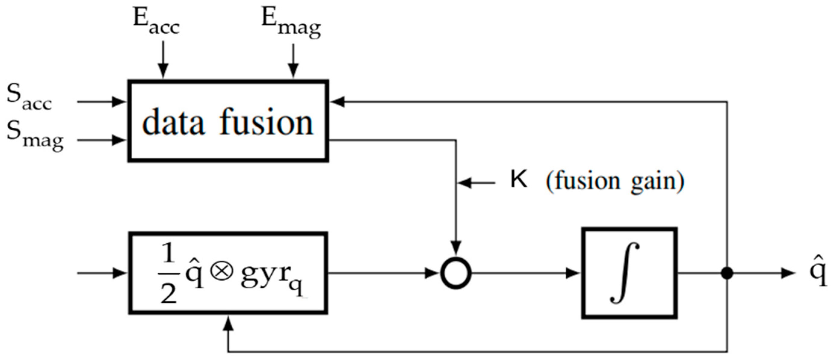
2.2. Attitude Estimation Principle
- Acceleration in provided by a three-axis accelerometer, noted , and its projection in , noted (g is the gravity).
- Earth’s magnetic field in provided by a magnetometer, noted , and its projection in , noted . , , and can be obtained using the World Magnetic Model (WMM) [40].
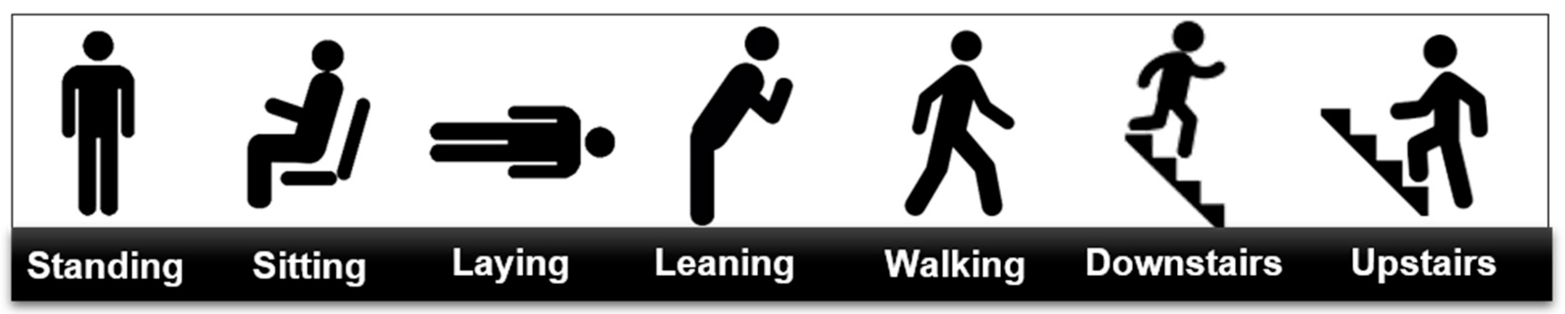
2.3. Sensors Placement and Studied Activities and Postures
- two modules placed on both feet,
- two modules on the thighs, and
- one module on the lower back.
2.4. Data Acquisition and Preparation
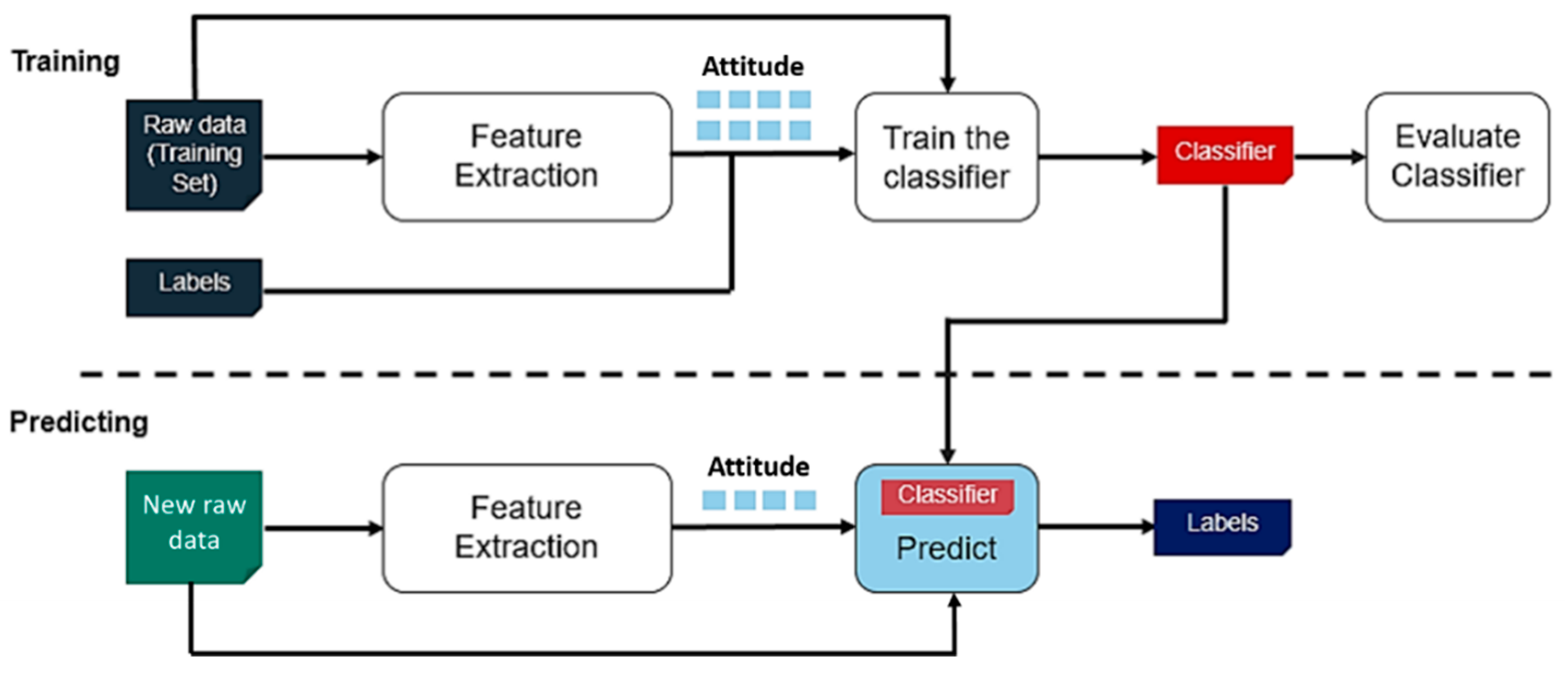
2.5. Overview of the Proposed Approach for HAR
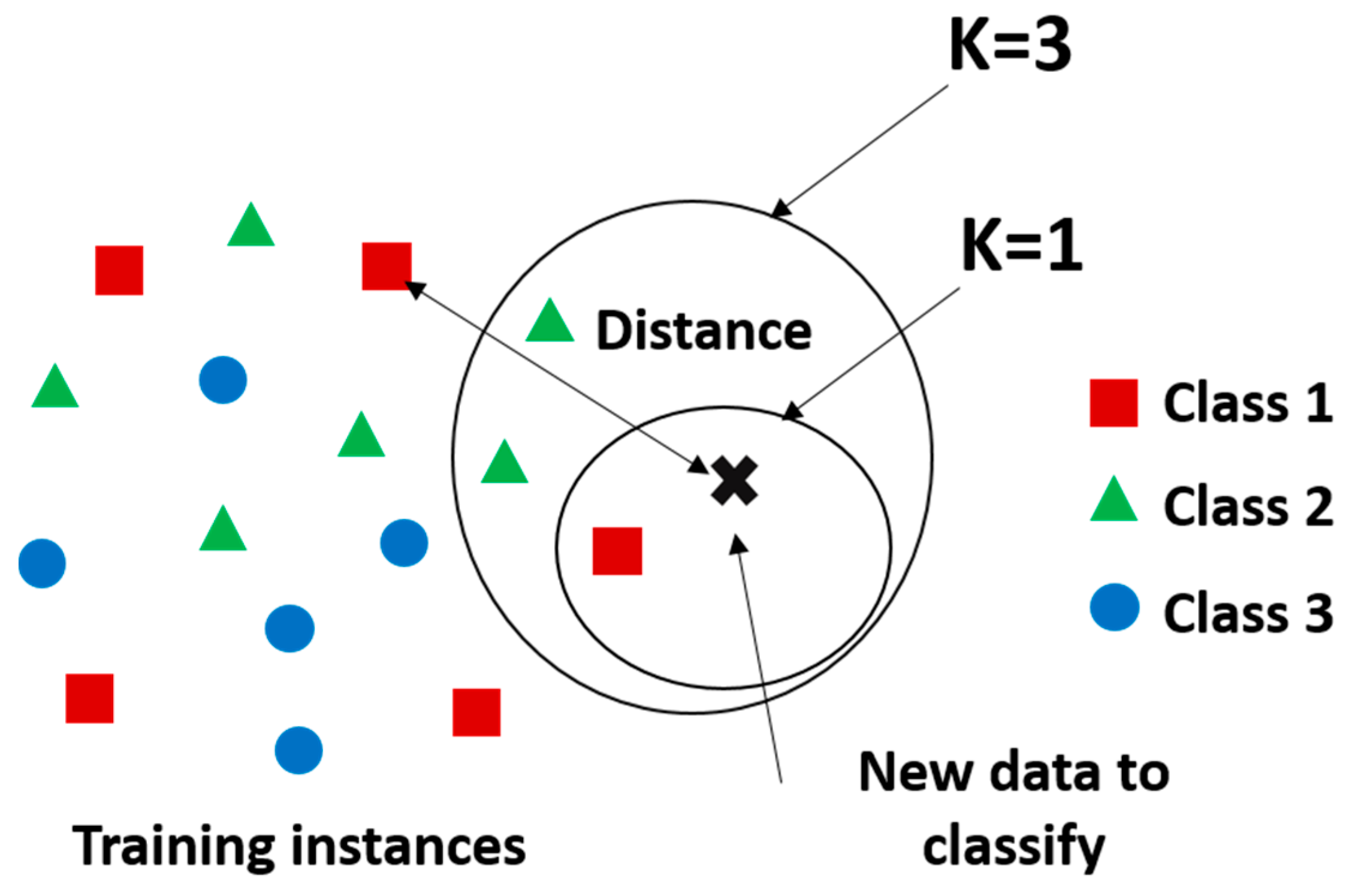
2.5.1. K-Nearest Neighbors Algorithm
- first it calculates d between and each training sample,
- then it estimates the conditional probability for each class bywhere is the set that contains the K points in the training data that are closest to , is the indicator function which equals 1 when the argument is true and 0 otherwise. Finally, our input gets assigned to the class with the largest probability.
2.5.2. Subspace KNN Algorithm
- Let N be the length of the training set, D be the number of its features and L be the number of individual models in the ensemble.
- For each individual model l, we choose nl (nl < N) to be the number of input points for l. It is common to have only one value of nl for all individual models.
- For each individual model l, we create a training set by selecting dl features from D with replacement and train the model.
- Finally, we combine the outputs of the L individual models using the majority vote. This vote outputs the class that has been chosen the most from all the different subspaces. The advantage of this method is that it enables us to have a different result for each subspace coming from the main training set, to later select the most recurrent one. This has been proven beneficial to avoid issues like overfitting [21,42].
3. Classification Results and Discussion for HAR
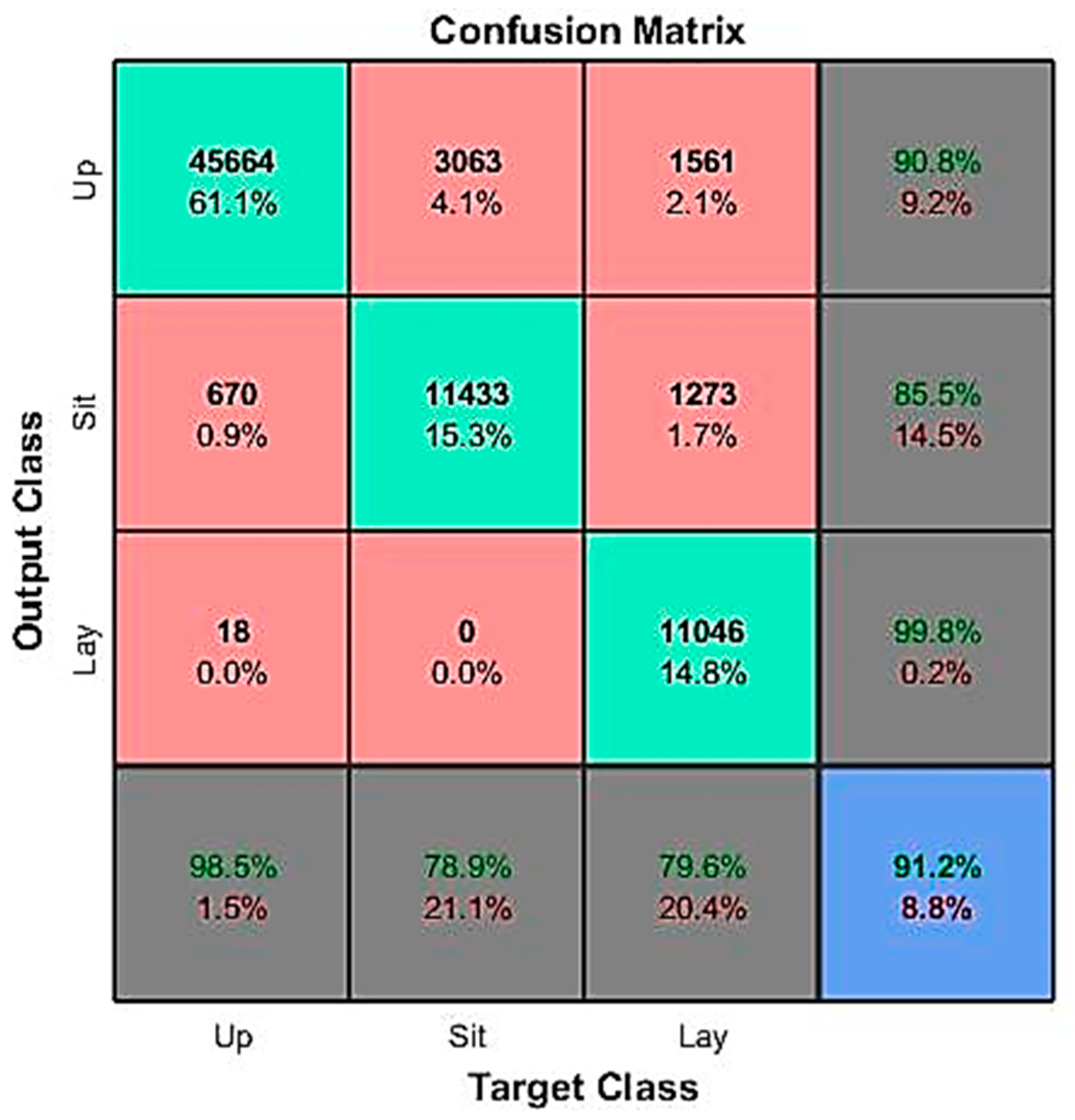
3.1. Confusion Matrix for Evaluation of Classification’s Performance
3.2. Results for Subspace KNN Algorithm with Raw Inertial Data Features
3.3. Results for Subspace KNN Algorithm with Attitude Features
3.3.1. Madgwick’s Filter for Attitude Estimation and Features Extraction
3.3.2. Results of Classification with Attitude-Based Features
3.4. Extended Discussion on Computation Time, Number of Features, and Accuracy
4. Conclusions
Author Contributions
Funding
Conflicts of Interest
References
- Cerón, J.; López, D.M. Human Activity Recognition Supported on Indoor Localization: A Systematic Review. Stud. Health Technol. Inf. 2018, 249, 93–101. [Google Scholar]
- Fu, B.; Kirchbuchner, F.; Kuijper, A.; Braun, A.; Vaithyalingam Gangatharan, D. Fitness Activity Recognition on Smartphones Using Doppler Measurements. Informatics 2018, 5, 24. [Google Scholar] [CrossRef]
- Sebestyen, G.; Stoica, I.; Hangan, A. Human activity recognition and monitoring for elderly people. In Proceedings of the IEEE 12th International Conference on Intelligent Computer Communication and Processing (ICCP), Cluj-Napoca, Romania, 8–10 September 2016; pp. 341–347. [Google Scholar]
- Taha, A.; Zayed, H.; Khalifa, M.E.; El-Horbarty, E.S. Human Activity Recognition for Surveillance Applications. In Proceedings of the ICIT 2015 The 7th International Conference on Information Technology, Amman, Jordan, 12–15 May 2015. [Google Scholar]
- Khattak, A.M.; Hung, D.V.; Truc, P.T.H.; Hung, L.X.; Guan, D.; Pervez, Z.; Han, M.; Lee, S.; Lee, Y.K. Context-aware Human Activity Recognition and decision making. In Proceedings of the 12th IEEE International Conference on e-Health Networking, Applications and Services, Lyon, France, 1–3 July 2010; pp. 112–118. [Google Scholar]
- Jia, Y. Diatetic and exercise therapy against diabetes mellitus. In Proceedings of the 2009 2th International Conference on Intelligent Networks and Intelligent Systems, Tianjin, China, 1–3 November 2009; pp. 693–696. [Google Scholar]
- Perez, A.J.; Labrador, M.A.; Barbeau, S.J. G-sense: A scalable architecture for global sensing and monitorin. IEEE Netw. 2010, 24, 57–64. [Google Scholar] [CrossRef]
- Turaga, P.; Chellappa, R.; Subrahmanian, V.S.; Udrea, O. Machine recognition of human activities: A survey. IEEE Trans. Circuits Syst. Video Technol. 2008, 18, 1473–1488. [Google Scholar] [CrossRef]
- Bayat, A.; Pomplun, M.; Tran, D.A. A study on human activity recognition using accelerometer data from smartphones. In Proceedings of the 11th International Conference on Mobile Systems and Pervasive Computing, Ontorio, ON, Canada, 17–20 August 2014. [Google Scholar]
- Ayu, M.A. Recognizing user activity based on accelerometer data from a mobile phone. In Proceedings of the IEEE Symposium on Computers & Informatics, Kuala Lumpur, Malaysia, 20–23 March 2011; pp. 617–621. [Google Scholar]
- Kaghyan, S. Activity recognition using k-nearest neighbor algorithm on smartphone with tri-axial accelerometer. Inf. Models Anal. 2012, 1, 146–156. [Google Scholar]
- Ponce, H. A Novel Wearable Sensor-Based Human Activity Recognition Approach Using Artificial Hydrocarbon Networks. Sensors 2016, 16, 1033. [Google Scholar] [CrossRef] [PubMed]
- Attal, F.; Mohammed, S.; Dedabrishvili, M.; Chamroukhi, F.; Oukhellou, L.; Amirat, Y. Physical Human Activity Recognition Using Wearable Sensors. Sensors 2015, 15, 31314–31338. [Google Scholar] [CrossRef] [PubMed] [Green Version]
- Soro, A.; Brunner, G.; Tanner, S.; Wattenhofer, R. Recognition and Repetition Counting for Complex Physical Exercises with Deep Learning. Sensors 2019, 19, 714. [Google Scholar] [CrossRef] [PubMed]
- Shoaib, M.; Bosch, S.; Incel, O.; Scholten, H.; Havinga, P. A survey of online activity recognition using mobile phones. Sensors 2015, 15, 2059–2085. [Google Scholar] [CrossRef] [PubMed]
- Cruz-Silva, N. Features Selection for Human Activity Recognition with iPhone Inertial Sensors. In Proceedings of the 16th Portuguese Conference on Artificial Inteligence, EPIA 2013, Angra do Heroísmo, Portugal, 9–12 September 2013. [Google Scholar]
- Sang, V.; Yano, S.; Kondo, T. On-Body Sensor Positions Hierarchical Classification. Sensors 2018, 18, 3612. [Google Scholar] [CrossRef] [PubMed]
- Mannini, A.; Sabatini, A.M. Machine learning methods for classifying human physical activity from on-body accelerometers. Sensors 2010, 10, 1154–1175. [Google Scholar] [CrossRef] [PubMed]
- Taborri, J.; Palermo, E.; Rossi, S. Automatic Detection of Faults in Race Walking: A Comparative Analysis of Machine-Learning Algorithms Fed with Inertial Sensor Data. Sensors 2019, 19, 1461. [Google Scholar] [CrossRef] [PubMed]
- Mandong, A.M.; Munir, U. Smartphone Based Activity Recognition using K-Nearest Neighbor Algorithm. In Proceedings of the International Conference on Engineering Technologies, Konya, Turkey, 26–28 October 2018. [Google Scholar]
- Janidarmian, M.; Roshan Fekr, A.; Radecka, K.; Zilic, Z. A Comprehensive Analysis on Wearable Acceleration Sensors in Human Activity Recognition. Sensors 2017, 17, 529. [Google Scholar] [CrossRef] [PubMed]
- Marín, J.; Vázquez, D.; López, A.M.; Amores, J.; Kuncheva, L.I. Occlusion handling via random subspace classifiers for human detection. IEEE Trans. Cybern. 2014, 44, 342–354. [Google Scholar] [CrossRef] [PubMed]
- Damaševičius, R.; Vasiljevas, M.; Šalkevičius, J.; Woźniak, M. Human Activity Recognition in AAL Environments Using Random Projections. Comput. Math. Methods Med. 2016, 2016, 1–17. [Google Scholar] [CrossRef] [PubMed] [Green Version]
- Wu, J.; Zhou, Z.; Fourati, H.; Cheng, Y. A Super Fast Attitude Determination Algorithm with Accelerometer and Magnetometer. IEEE Trans. Consum. Electron. 2018, 64, 375–381. [Google Scholar] [CrossRef]
- Michel, T.; Geneves, P.; Fourati, H.; Layaïda, N. Attitude estimation for indoor navigation and augmented reality with smartphones. Pervasive Mob. Comput. 2018, 46, 96–121. [Google Scholar] [CrossRef] [Green Version]
- Gait Up. Startup for Fast and Accurate Motion Analysis. Available online: https://gaitup.com/ (accessed on 20 April 2018).
- Kuipers, B.K. Quaternions and Rotation Sequences; Princeton University Press: Princeton, NJ, USA, 1998. [Google Scholar]
- Rotations in Three-Dimensions: Euler Angles and Rotation Matrices. Available online: http://danceswithcode.net/engineeringnotes/rotations_in_3d/rotations_in_3d_part1.html (accessed on 23 April 2018).
- Wahba, G. A least squares estimate of satellite attitude. SIAM Rev. 1965, 7, 409. [Google Scholar] [CrossRef]
- Black, H.D. A passive system for determining the attitude of a satellite. AIAA J. 1964, 2, 1350–1351. [Google Scholar] [CrossRef]
- Shuster, M.D. Three-axis attitude determination from vector observations. J. Guid. Control. Dyn. 1981, 4, 70–77. [Google Scholar] [CrossRef]
- Markley, F. Attitude determination using vector observations and the singular value decomposition. J. Astronaut. Sci. 1988, 36, 1245–25871. [Google Scholar]
- Choukroun, D.; Bar-itzhack, I.Y.; Oshman, Y. A Novel Quaternion Kalman Filter. IEEE Trans. Aerosp. Electron. Syst. 2006, 42, 174–190. [Google Scholar] [CrossRef]
- Bernal-Polo, P.; Martínez-Barberá, H. Kalman Filtering for Attitude Estimation with Quaternions and Concepts from Manifold Theory. Sensors 2019, 19, 149. [Google Scholar] [CrossRef] [PubMed]
- Harada, T. Portable absolute orientation estimation device with wireless network under accelerated situation. In Proceedings of the International Conference on Robotics and Automation, New Orleans, LA, USA, 26 April–1 May 2004. [Google Scholar]
- Fourati, H. Heterogeneous Data Fusion Algorithm for Pedestrian Navigation via Foot-Mounted Inertial Measurement Unit and Complementary Filter. IEEE Trans. Instrum. Meas. 2015, 64, 221–229. [Google Scholar] [CrossRef]
- Martin, P. Design and implementation of a low-cost observer based attitude and heading reference system. Control. Eng. Pract. 2010, 18, 712–722. [Google Scholar] [CrossRef]
- Markley, F. Quaternions attitude estimation using vector observations. J. Astronaut. Sci. 2000, 48, 359–380. [Google Scholar]
- Michel, T. On attitude estimation with smartphones. In Proceedings of the IEEE International Conference on Pervasive Computing and Communications, Kona, HI, USA, 13–17 March 2017. [Google Scholar]
- NOAA. The World Magnetic Model. Available online: http://www.ngdc.noaa.gov (accessed on 20 April 2018).
- Altman, N.S. An introduction to kernel and nearest-neighbor nonparametric regression. Am. Stat. 1992, 46, 175–185. [Google Scholar]
- Ho, T.K. The random subspace method for constructing decision forests. IEEE Trans. Pattern Anal. Mach. Intell. 1998, 20, 832–844. [Google Scholar]
- Madgwick, S.O.H. An. Efficient Orientation Filter for Inertial and Inertial/Magnetic Sensor Arrays; Report x-io; University of Bristol: Bristol, UK, 2010. [Google Scholar]


| Subject | 1 | 2 | 3 | 4 | 5 | 6 | 7 | 8 |
|---|---|---|---|---|---|---|---|---|
| Age (years) | 19 | 33 | 22 | 38 | 46 | 27 | 25 | 23 |
| Weight (kg) | 53 | 85 | 79 | 86 | 85 | 65 | 90 | 69 |
| Height (m) | 1.65 | 1.77 | 1.78 | 1.79 | 1.82 | 1.67 | 1.85 | 1.58 |
| Protocol 1 | Protocol 2 | Protocol 3 |
|---|---|---|
| Jumping jacks (2 times) | Wait (30 s) | Wait (30 s) |
| Sitting (1 min) | Walk (1 min) | Go up the stairs (11 steps) |
| Jumping jacks (2 times) | Wait (30 s) | Turn and wait (30 s) |
| Standing up (1 min) | Run (1 min) | Go down the stairs (11 steps) |
| Jumping jacks (2 times) | Wait (30 s) | Turn |
| Wait (30 s) | Jump (10 times) | Repeat this loop (5 times) |
| Repeat this loop (5 times) | Repeat this loop (5 times) | |
| Jumping jacks (2 times) | ||
| Laying on the ground (1 min) | ||
| Jumping jacks (2 times) | ||
| Standing up (1 min) | ||
| Jumping jacks (2 times) | ||
| Wait (30 s) | ||
| Repeat this loop (5 times) |
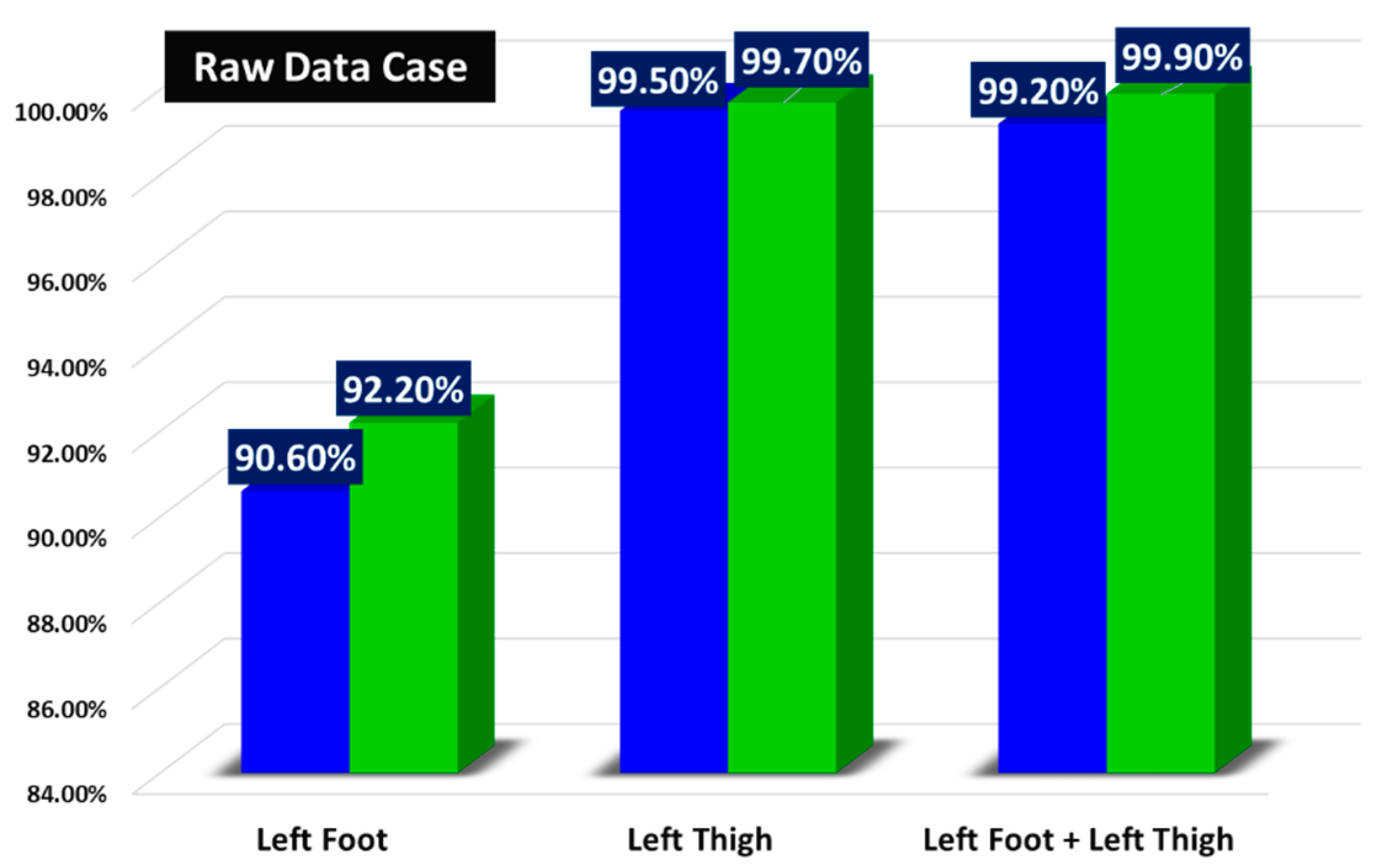
| Locations | LB | LF | LT | LF + LT | LF + LT + LB |
|---|---|---|---|---|---|
| Accuracy (%) | 80.1 | 89.9 | 88.6 | 92.2 | 92.9 |
| Overall Accuracy (%) | Raw Data | 80.1 |
| Euler Angles | 80.3 | |
| Quaternion | 87.9 |
© 2019 by the authors. Licensee MDPI, Basel, Switzerland. This article is an open access article distributed under the terms and conditions of the Creative Commons Attribution (CC BY) license (http://creativecommons.org/licenses/by/4.0/).
Share and Cite
Zmitri, M.; Fourati, H.; Vuillerme, N. Human Activities and Postures Recognition: From Inertial Measurements to Quaternion-Based Approaches. Sensors 2019, 19, 4058. https://doi.org/10.3390/s19194058
Zmitri M, Fourati H, Vuillerme N. Human Activities and Postures Recognition: From Inertial Measurements to Quaternion-Based Approaches. Sensors. 2019; 19(19):4058. https://doi.org/10.3390/s19194058
Chicago/Turabian StyleZmitri, Makia, Hassen Fourati, and Nicolas Vuillerme. 2019. "Human Activities and Postures Recognition: From Inertial Measurements to Quaternion-Based Approaches" Sensors 19, no. 19: 4058. https://doi.org/10.3390/s19194058
APA StyleZmitri, M., Fourati, H., & Vuillerme, N. (2019). Human Activities and Postures Recognition: From Inertial Measurements to Quaternion-Based Approaches. Sensors, 19(19), 4058. https://doi.org/10.3390/s19194058