Toward High-Resolution Soil Moisture Monitoring by Combining Active-Passive Microwave and Optical Vegetation Remote Sensing Products with Land Surface Model


Abstract
:
1. Introduction
2. Study Area and Datasets
2.1. Study Areas and In-Situ Observations
2.2. Datasets
3. Methods
3.1. Land Surface Model
3.2. Radiative Transfer Model
3.3. Parameter Optimization Scheme
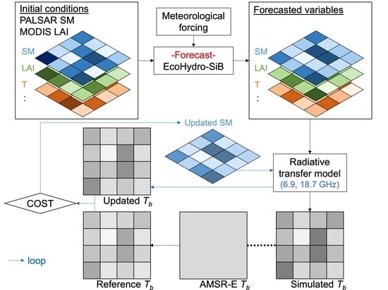
3.4. Assimilation Scheme
3.5. Experimental Design
4. Results
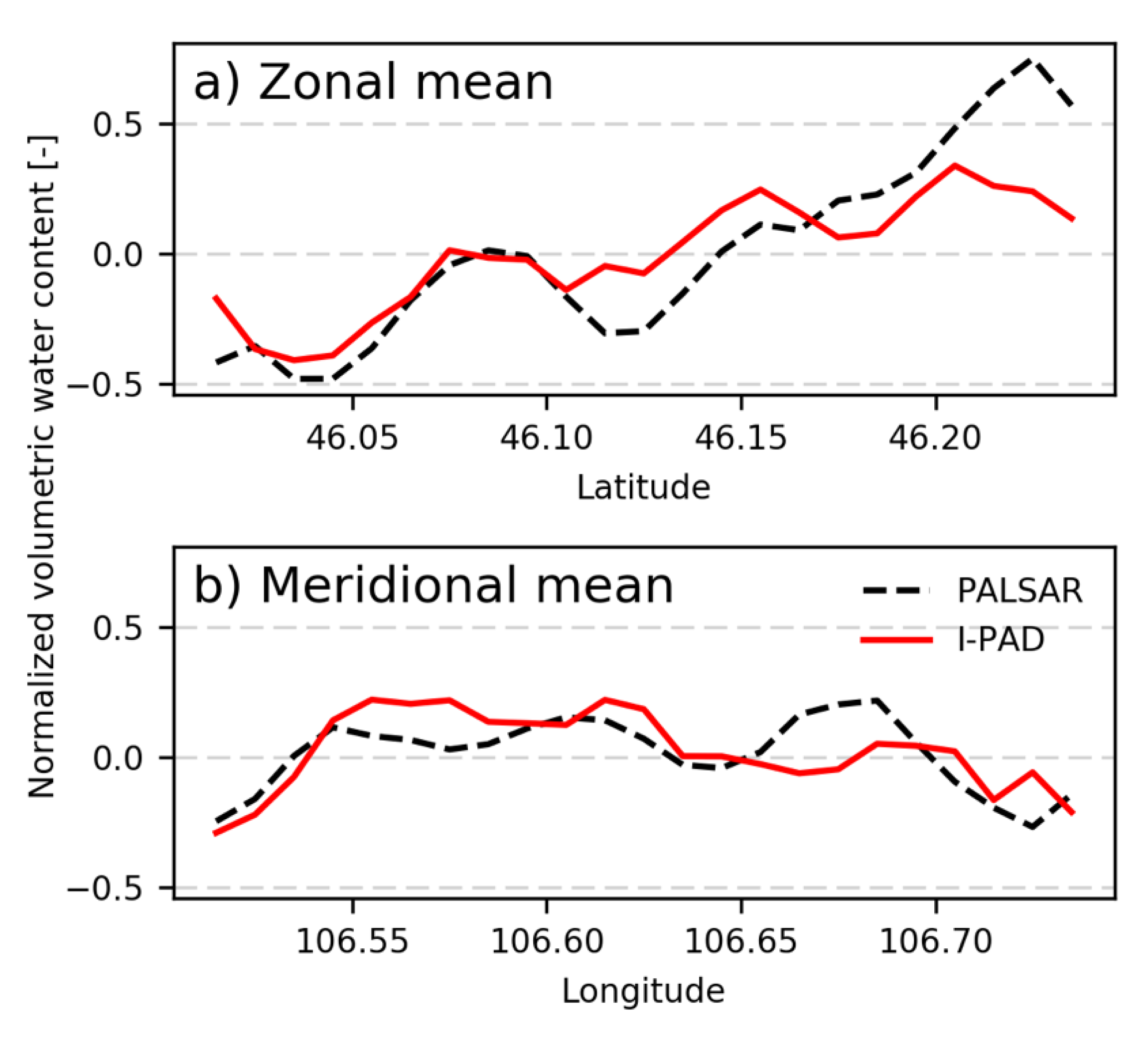
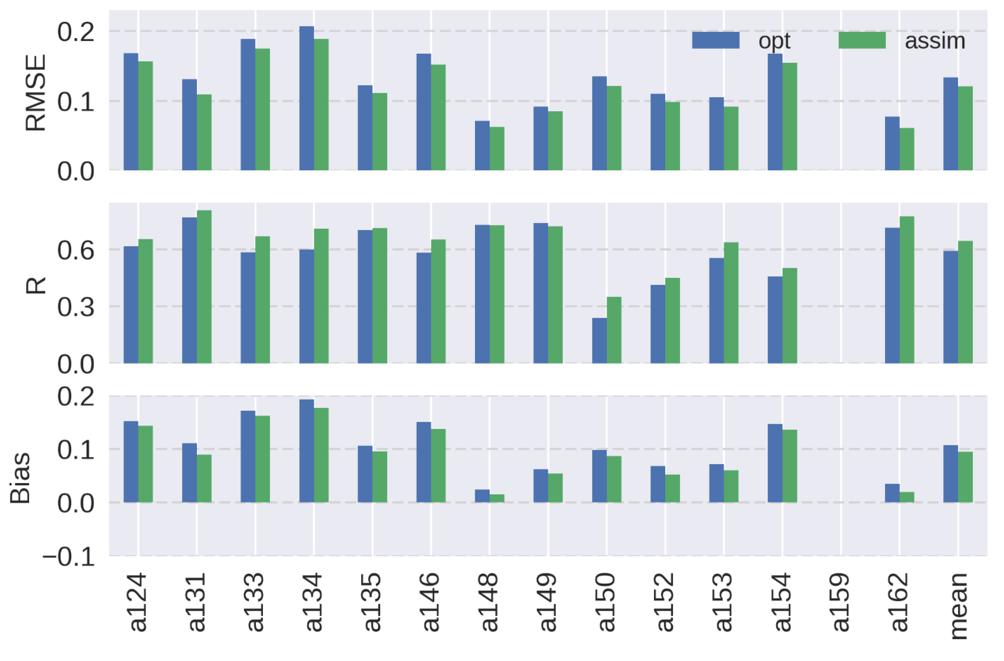
4.1. Mongolia
4.2. Little Washita
5. Discussion
6. Conclusions
Author Contributions
Funding
Acknowledgments
Conflicts of Interest
Appendix A
Appendix B

References
- Western, A.W.; Grayson, R.B.; Blöschl, G. Scaling of Soil Moisture: A Hydrologic Perspective. Annu. Rev. Earth Planet. Sci. 2002, 30, 149–180. [Google Scholar] [CrossRef] [Green Version]
- Koster, R.D. Regions of Strong Coupling Between Soil Moisture and Precipitation. Science 2004, 305, 1138–1140. [Google Scholar] [CrossRef] [PubMed] [Green Version]
- Seneviratne, S.I.; Corti, T.; Davin, E.L.; Hirschi, M.; Jaeger, E.B.; Lehner, I.; Orlowsky, B.; Teuling, A.J. Investigating soil moisture–climate interactions in a changing climate: A review. Earth Sci. Rev. 2010, 99, 125–161. [Google Scholar] [CrossRef]
- Famiglietti, J.S.; Rudnicki, J.W.; Rodell, M. Variability in surface moisture content along a hillslope transect: Rattlesnake Hill, Texas. J. Hydrol. 1998, 210, 259–281. [Google Scholar] [CrossRef] [Green Version]
- Teuling, A.J. Improved understanding of soil moisture variability dynamics. Geophys. Res. Lett. 2005, 32, L05404. [Google Scholar] [CrossRef]
- Rosenbaum, U.; Bogena, H.R.; Herbst, M.; Huisman, J.A.; Peterson, T.J.; Weuthen, A.; Western, A.W.; Vereecken, H. Seasonal and event dynamics of spatial soil moisture patterns at the small catchment scale. Water Resour. Res. 2012, 48. [Google Scholar] [CrossRef] [Green Version]
- Sabaghy, S.; Walker, J.P.; Renzullo, L.J.; Jackson, T.J. Spatially enhanced passive microwave derived soil moisture: Capabilities and opportunities. Remote Sens. Environ. 2018, 209, 551–580. [Google Scholar] [CrossRef]
- Schmugge, T.; O’Neill, P.; Wang, J. Passive Microwave Soil Moisture Research. IEEE Trans. Geosci. Remote Sens. 1986, GE-24, 12–22. [Google Scholar] [CrossRef]
- Dobson, M.C.; Ulaby, F.T. Active Microwave Soil Moisture Research. IEEE Trans. Geosci. Remote Sens. 1986, GE-24, 23–36. [Google Scholar] [CrossRef]
- Chauhan, N.S.; Miller, S.; Ardanuy, P. Spaceborne soil moisture estimation at high resolution: A microwave-optical/IR synergistic approach. Int. J. Remote Sens. 2003, 24, 4599–4622. [Google Scholar] [CrossRef]
- Merlin, O.; Rüdiger, C.; Al Bitar, A.; Richaume, P.; Walker, J.P.; Kerr, Y.H. Disaggregation of SMOS soil moisture in Southeastern Australia. IEEE Trans. Geosci. Remote Sens. 2012, 50, 1556–1571. [Google Scholar] [CrossRef]
- Kim, G.; Barros, A.P. Downscaling of remotely sensed soil moisture with a modified fractal interpolation method using contraction mapping and ancillary data. Remote Sens. Environ. 2002, 83, 400–413. [Google Scholar] [CrossRef]
- de Jeu, R.A.M.; Holmes, T.R.H.; Parinussa, R.M.; Owe, M. A spatially coherent global soil moisture product with improved temporal resolution. J. Hydrol. 2014, 516, 284–296. [Google Scholar] [CrossRef]
- Wagner, W.; Hahn, S.; Kidd, R.; Melzer, T.; Bartalis, Z.; Hasenauer, S.; Figa-Saldaña, J.; De Rosnay, P.; Jann, A.; Schneider, S.; et al. The ASCAT soil moisture product: A review of its specifications, validation results, and emerging applications. Meteorol. Z. 2013, 22, 5–33. [Google Scholar] [CrossRef]
- Entekhabi, D.; Njoku, E.G.; O’Neill, P.E.; Kellogg, K.H.; Crow, W.T.; Edelstein, W.N.; Entin, J.K.; Goodman, S.D.; Jackson, T.J.; Johnson, J.; et al. The Soil Moisture Active Passive (SMAP) Mission. Proc. IEEE 2010, 98, 704–716. [Google Scholar] [CrossRef]
- Das, N.N.; Entekhabi, D.; Njoku, E.G.; Shi, J.J.C.; Johnson, J.T.; Colliander, A. Tests of the SMAP Combined Radar and Radiometer Algorithm Using Airborne Field Campaign Observations and Simulated Data. IEEE Trans. Geosci. Remote Sens. 2014, 52, 2018–2028. [Google Scholar] [CrossRef]
- Das, N.N.; Entekhabi, D.; Dunbar, R.S.; Colliander, A.; Chen, F.; Crow, W.; Jackson, T.J.; Berg, A.; Bosch, D.D.; Caldwell, T.; et al. The SMAP mission combined active-passive soil moisture product at 9 km and 3 km spatial resolutions. Remote Sens. Environ. 2018, 211, 204–217. [Google Scholar] [CrossRef]
- Bindlish, R.; Barros, A.P. Subpixel variability of remotely sensed soil moisture: An inter-comparison study of SAR and ESTAR. IEEE Trans. Geosci. Remote Sens. 2002, 40, 326–337. [Google Scholar] [CrossRef]
- Narayan, U.; Lakshmi, V.; Jackson, T.J. High-resolution change estimation of soil moisture using L-band radiometer and Radar observations made during the SMEX02 experiments. IEEE Trans. Geosci. Remote Sens. 2006, 44, 1545–1554. [Google Scholar] [CrossRef]
- Montzka, C.; Jagdhuber, T.; Horn, R.; Bogena, H.R.; Hajnsek, I.; Reigber, A.; Vereecken, H. Investigation of SMAP Fusion Algorithms With Airborne Active and Passive L-Band Microwave Remote Sensing. IEEE Trans. Geosci. Remote Sens. 2016, 54, 3878–3889. [Google Scholar] [CrossRef]
- Santi, E.; Paloscia, S.; Pettinato, S.; Brocca, L.; Ciabatta, L.; Entekhabi, D. On the synergy of SMAP, AMSR2 AND SENTINEL-1 for retrieving soil moisture. Int. J. Appl. Earth Obs. Geoinf. 2018, 65, 114–123. [Google Scholar] [CrossRef]
- Draper, C.S.; Reichle, R.H.; De Lannoy, G.J.M.; Liu, Q. Assimilation of passive and active microwave soil moisture retrievals. Geophys. Res. Lett. 2012, 39. [Google Scholar] [CrossRef] [Green Version]
- Kolassa, J.; Reichle, R.H.; Draper, C.S. Merging active and passive microwave observations in soil moisture data assimilation. Remote Sens. Environ. 2017, 191, 117–130. [Google Scholar] [CrossRef]
- Lievens, H.; Reichle, R.H.; Liu, Q.; De Lannoy, G.J.M.; Dunbar, R.S.; Kim, S.B.; Das, N.N.; Cosh, M.; Walker, J.P.; Wagner, W. Joint Sentinel-1 and SMAP data assimilation to improve soil moisture estimates. Geophys. Res. Lett. 2017, 44, 6145–6153. [Google Scholar] [CrossRef]
- Geudtner, D. Sentinel-1 system overview and performance. In Proceedings of the 2012 IEEE International Geoscience and Remote Sensing Symposium, Munich, Germany, 22–27 July 2012; Volume 852802, pp. 1719–1721. [Google Scholar]
- Sahoo, A.K.; De Lannoy, G.J.M.; Reichle, R.H.; Houser, P.R. Assimilation and downscaling of satellite observed soil moisture over the Little River Experimental Watershed in Georgia, USA. Adv. Water Resour. 2013, 52, 19–33. [Google Scholar] [CrossRef]
- Draper, C.; Reichle, R. The impact of near-surface soil moisture assimilation at subseasonal, seasonal, and inter-annual timescales. Hydrol. Earth Syst. Sci. 2015, 19, 4831–4844. [Google Scholar] [CrossRef] [Green Version]
- Reichle, R.H.; De Lannoy, G.J.M.; Liu, Q.; Ardizzone, J.V.; Colliander, A.; Conaty, A.; Crow, W.; Jackson, T.J.; Jones, L.A.; Kimball, J.S.; et al. Assessment of the SMAP Level-4 Surface and Root-Zone Soil Moisture Product Using In Situ Measurements. J. Hydrometeorol. 2017, 18, 2621–2645. [Google Scholar] [CrossRef]
- Sawada, Y.; Koike, T.; Walker, J.P. A land data assimilation system for simultaneous simulation of soil moisture and vegetation dynamics. J. Geophys. Res. Atmos. 2015, 120, 5910–5930. [Google Scholar] [CrossRef]
- Kaihotsu, I.; Yamanaka, T.; Koike, T.; Oyunbaatar, D.; Davaa, G. Ground truth for evaluation of soil moisture and geophysical/vegetation parameters related to ground surface conditions with AMSR and GLI in the Mongolian Plateau. Available online: https://www.researchgate.net/publication/288256285_Ground_truth_for_evaluation_of_soil_moisture_and_geophysicalvegetation_parameters_related_to_ground_surface_conditions_with_AMSR_and_GLI_in_the_Mongolian_Plateau_ground-based_observations_for_the_ADEO (accessed on 11 September 2019).
- Kaihotsu, I.; Koike, T.; Yamanaka, T.; Fujii, H.; Ohta, T.; Tamagawa, K.; Oyunbaatar, D.; Akiyama, R. Validation of Soil Moisture Estimation by AMSR-E in the Mongolian Plateau. J. Remote Sens. Soc. Jpn. 2009, 29, 271–281. [Google Scholar]
- Starks, P.J.; Fiebrich, C.A.; Grimsley, D.L.; Garbrecht, J.D.; Steiner, J.L.; Guzman, J.A.; Moriasi, D.N. Upper Washita River Experimental Watersheds: Meteorologic and Soil Climate Measurement Networks. J. Environ. Qual. 2014, 43, 1239. [Google Scholar] [CrossRef]
- Brock, F.V.; Crawford, K.C.; Elliott, R.L.; Cuperus, G.W.; Stadler, S.J.; Johnson, H.L.; Eilts, M.D. The Oklahoma Mesonet: A Technical Overview. J. Atmos. Ocean. Technol. 1995, 12, 5–19. [Google Scholar] [CrossRef]
- McPherson, R.A.; Fiebrich, C.A.; Crawford, K.C.; Kilby, J.R.; Grimsley, D.L.; Martinez, J.E.; Basara, J.B.; Illston, B.G.; Morris, D.A.; Kloesel, K.A.; et al. Statewide Monitoring of the Mesoscale Environment: A Technical Update on the Oklahoma Mesonet. J. Atmos. Ocean. Technol. 2007, 24, 301–321. [Google Scholar] [CrossRef] [Green Version]
- Cosh, M.H.; Evett, S.R.; McKee, L. Surface soil water content spatial organization within irrigated and non-irrigated agricultural fields. Adv. Water Resour. 2012, 50, 55–61. [Google Scholar] [CrossRef]
- Shepard, D. A two-dimensional interpolation function for irregularly-spaced data. In Proceedings of the 1968 23rd ACM National Conference, New York, NY, USA, 27–29 August 1968; ACM Press: New York, NY, USA, 1968; pp. 517–524. [Google Scholar]
- Aida, K.; Koike, T.; Kaihotsu, I. Study on Development of a Frequently Applicable SAR Algorithm for Soil Moisture Using ALOS/PALSAR. J. Jpn. Soc. Civ. Eng. Ser. B1 Hydraul. Eng. 2014, 70, I_589–I_594. [Google Scholar]
- Sawada, Y.; Koike, T. Simultaneous estimation of both hydrological and ecological parameters in an ecohydrological model by assimilating microwave signal. J. Geophys. Res. Atmos. 2014, 119, 8839–8857. [Google Scholar] [CrossRef]
- Koike, T.; Nakamura, Y.; Kaihotsu, I.; Davva, G.; Matsuura, N.; Tamagawa, K.; Fujii, H. Development of an Advanced Microwave Scanning Radiometer (AMSR-E) Algorithm of Soil Moisture and Vegetation Water Content. Annu. J. Hydraul. Eng. 2004, 48, 217–222. [Google Scholar] [CrossRef]
- Rodell, M.; Houser, P.R.; Jambor, U.; Gottschalck, J.; Mitchell, K.; Meng, C.-J.; Arsenault, K.; Cosgrove, B.; Radakovich, J.; Bosilovich, M.; et al. The Global Land Data Assimilation System. Bull. Am. Meteorol. Soc. 2004, 85, 381–394. [Google Scholar] [CrossRef] [Green Version]
- Xia, Y.; Mitchell, K.; Ek, M.; Sheffield, J.; Cosgrove, B.; Wood, E.; Luo, L.; Alonge, C.; Wei, H.; Meng, J.; et al. Continental-scale water and energy flux analysis and validation for the North American Land Data Assimilation System project phase 2 (NLDAS-2): 1. Intercomparison and application of model products. J. Geophys. Res. Atmos. 2012, 117. [Google Scholar] [CrossRef]
- Xia, Y.; Mitchell, K.; Ek, M.; Cosgrove, B.; Sheffield, J.; Luo, L.; Alonge, C.; Wei, H.; Meng, J.; Livneh, B.; et al. Continental-scale water and energy flux analysis and validation for North American Land Data Assimilation System project phase 2 (NLDAS-2): 2. Validation of model-simulated streamflow. J. Geophys. Res. Atmos. 2012, 117. [Google Scholar] [CrossRef]
- Sawada, Y.; Koike, T. Towards ecohydrological drought monitoring and prediction using a land data assimilation system: A case study on the Horn of Africa drought (2010–2011). J. Geophys. Res. Atmos. 2016, 121, 8229–8242. [Google Scholar] [CrossRef]
- Yang, K.; Koike, T.; Kaihotsu, I.; Qin, J. Validation of a Dual-Pass Microwave Land Data Assimilation System for Estimating Surface Soil Moisture in Semiarid Regions. J. Hydrometeorol. 2009, 10, 780–793. [Google Scholar] [CrossRef] [Green Version]
- Sawada, Y.; Koike, T.; Jaranilla-Sanchez, P.A. Modeling hydrologic and ecologic responses using a new eco-hydrological model for identification of droughts. Water Resour. Res. 2014, 50, 6214–6235. [Google Scholar] [CrossRef]
- Kuria, D.N.; Koike, T.; Lu, H.; Tsutsui, H.; Graf, T. Field-Supported Verification and Improvement of a Passive Microwave Surface Emission Model for Rough, Bare, and Wet Soil Surfaces by Incorporating Shadowing Effects. IEEE Trans. Geosci. Remote Sens. 2007, 45, 1207–1216. [Google Scholar] [CrossRef]
- Wang, L.; Koike, T.; Yang, D.; Yang, K. Improving the hydrology of the Simple Biosphere Model 2 and its evaluation within the framework of a distributed hydrological model. Hydrol. Sci. J. 2009, 54, 989–1006. [Google Scholar] [CrossRef] [Green Version]
- Sawada, Y.; Koike, T. Ecosystem resilience to the Millennium drought in southeast Australia (2001–2009). J. Geophys. Res. Biogeosci. 2016, 121, 2312–2327. [Google Scholar] [CrossRef]
- van Genuchten, M.T. A Closed-form Equation for Predicting the Hydraulic Conductivity of Unsaturated Soils1. Soil Sci. Soc. Am. J. 1980, 44, 892. [Google Scholar] [CrossRef]
- Mo, T.; Choudhury, B.J.; Schmugge, T.J.; Wang, J.R.; Jackson, T.J. A model for microwave emission from vegetation-covered fields. J. Geophys. Res. 1982, 87, 11229. [Google Scholar] [CrossRef]
- Duan, Q.; Sorooshian, S.; Gupta, V. Effective and efficient global optimization for conceptual rainfall-runoff models. Water Resour. Res. 1992, 28, 1015–1031. [Google Scholar] [CrossRef]
- Drusch, M.; Wood, E.F.; Simmer, C. Up-scaling effects in passive microwave remote sensing: ESTAR 1.4 GHz measurements during SGP ’97. Geophys. Res. Lett. 1999, 26, 879–882. [Google Scholar] [CrossRef]
- Reichle, R.H.; Entekhabi, D.; McLaughlin, D.B.B.; Parsons, R.M. Downscaling of radio brightness measurements for soil moisture estimation: A four-dimensional variational data assimilation approach. Water Resour. Res. 2001, 37, 2353–2364. [Google Scholar] [CrossRef] [Green Version]
- Wang, L.; Koike, T.; Yang, K.; Jackson, T.J.; Bindlish, R.; Yang, D. Development of a distributed biosphere hydrological model and its evaluation with the Southern Great Plains experiments (SGP97 and SGP99). J. Geophys. Res. Atmos. 2009, 114, 1–15. [Google Scholar] [CrossRef]
- Crow, W.T.; Berg, A.A.; Cosh, M.H.; Loew, A.; Mohanty, B.P.; Panciera, R.; de Rosnay, P.; Ryu, D.; Walker, J.P. Upscaling sparse ground-based soil moisture observations for the validation of coarse-resolution satellite soil moisture products. Rev. Geophys. 2012, 50, 1–20. [Google Scholar] [CrossRef]
- Sawada, Y.; Koike, T.; Aida, K.; Toride, K.; Walker, J.P. Fusing Microwave and Optical Satellite Observations to Simultaneously Retrieve Surface Soil Moisture, Vegetation Water Content, and Surface Soil Roughness. IEEE Trans. Geosci. Remote Sens. 2017, 55, 6195–6206. [Google Scholar] [CrossRef]
- Sawada, Y.; Tsutsui, H.; Koike, T.; Rasmy, M.; Seto, R.; Fujii, H. A Field Verification of an Algorithm for Retrieving Vegetation Water Content From. IEEE Trans. Geosci. Remote Sens. 2016, 54, 2082–2095. [Google Scholar] [CrossRef]
- Yamamoto, M.K.; Shige, S. Implementation of an orographic/nonorographic rainfall classification scheme in the GSMaP algorithm for microwave radiometers. Atmos. Res. 2015, 163, 36–47. [Google Scholar] [CrossRef]
- Fung, A.K.; Li, Z.; Chen, K.S. Backscattering from a randomly rough dielectric surface. IEEE Trans. Geosci. Remote Sens. 1992, 30, 356–369. [Google Scholar] [CrossRef]
- Tsang, L. Dense media radiative transfer theory for dense discrete random media with particles of multiple sizes and permittivities. Prog. Electromagn. Res. 1992, 6, 181–225. [Google Scholar]
- Ulander, L.M.H. Radiometric slope correction of synthetic-aperture radar images. IEEE Trans. Geosci. Remote Sens. 1996, 34, 1115–1122. [Google Scholar] [CrossRef]


| Site | PALSAR Observations |
|---|---|
| Mongolia | 21 July 2009, 5 September 2009, 8 June 2010, 23 July 2010 |
| Little Washita | 6 February 2007, 25 February 2007, 2 March 2007 |
© 2019 by the authors. Licensee MDPI, Basel, Switzerland. This article is an open access article distributed under the terms and conditions of the Creative Commons Attribution (CC BY) license (http://creativecommons.org/licenses/by/4.0/).
Share and Cite
Toride, K.; Sawada, Y.; Aida, K.; Koike, T. Toward High-Resolution Soil Moisture Monitoring by Combining Active-Passive Microwave and Optical Vegetation Remote Sensing Products with Land Surface Model. Sensors 2019, 19, 3924. https://doi.org/10.3390/s19183924
Toride K, Sawada Y, Aida K, Koike T. Toward High-Resolution Soil Moisture Monitoring by Combining Active-Passive Microwave and Optical Vegetation Remote Sensing Products with Land Surface Model. Sensors. 2019; 19(18):3924. https://doi.org/10.3390/s19183924
Chicago/Turabian StyleToride, Kinya, Yohei Sawada, Kentaro Aida, and Toshio Koike. 2019. "Toward High-Resolution Soil Moisture Monitoring by Combining Active-Passive Microwave and Optical Vegetation Remote Sensing Products with Land Surface Model" Sensors 19, no. 18: 3924. https://doi.org/10.3390/s19183924