1. Introduction
In the context of high pressure and high temperature flow rigs, flow patterns are investigated. Tomography is a suitable technique for its applicability and non-intrusiveness. This imaging technique is used to reconstruct the volume of an object from measurements of penetrating waves or particles on its external boundary. Tomography is based on measurements of the boundary conditions of a system, where both the signal emitter and receiver have to be well known in space. Various tomography techniques exist using electromagnetic, acoustic waves, or electron and muon particles. Among the use of tomography in applications, the most well established is medical imaging using X-ray-based CT scans or electromagnetic waves in magnetic resonance imaging. Nevertheless, these techniques are not robust in this context, complex to implement, and expensive.
Electrical Impedance Tomography (EIT) [
1,
2,
3,
4] is another tomographic method that consists of imposing (resp. measuring) an electrical current passing through a set of electrodes at the surface of a body, while measuring (resp. imposing) the electrical potential over another set of electrodes. This technique is preferred for its applicability at high pressure and temperature, robustness, and relatively low cost. The standard approach of EIT is based on the concept of Time-Division Multiplexing (TDM), where the excitation signal is routed to a single pair of electrodes at any given time. The sequential selection of these pairs of electrodes with multiplexers or electronic switching [
5] creates an excitation strategy and builds an EIT data frame, which includes the measurement data for all excitation pairs. The EIT data frame defines the Neumann and Dirichlet boundary conditions to be used in the associated inverse problem of reconstructing the electrical conductivity field inside the body.
EIT necessitates potentially a high data-frame acquisition rate, for instance in flow study involving rapidly-evolving flow regimes [
6,
7]. The challenge is that increasing the number of frames per seconds (fps) reduces the measurement time, while a large number of measurements is required to limit the ill-posedness of the inverse problem. In addition, the sequential excitation of the electrodes in contact with ionic solutions results in significant difficulties caused by transient voltages due to the presence of capacitive components in the electrode–electrolyte interface [
8]. Therefore, the TDM sequential measurement procedure requires dead time, complex signal processing techniques, or hardware improvement to limit the effects of contact impedance [
9,
10].
Several high-speed EIT systems of hundreds of fps have been proposed in the literature. In [
11], a multichannel architecture system was presented, containing a control module that manages and synchronizes 64 channels capable of generating and measuring voltages and currents. The system was able to collect 182 frames per seconds when acquiring 15 spatial patterns with a Signal-to-Noise Ratio (SNR) from 65.5–96 dB when averaging the signal from 32 samples. Another EIT system proposed in [
12] allows capturing over 100 frames per seconds with an SNR greater than 90 dB when averaging the signal. Concerning Electrical Capacitance Tomography (ECT), another soft field imaging technique, several systems were also reported in [
13,
14,
15] with high frame rate. Furthermore, an EIT system was developed in our group [
16] to reach the Data Acquisition (DAQ) rate of 833 fps when acquiring 120 spatial patterns with TDM. Nevertheless, in any case, high speed is reached at the price of a small number of electrodes, a partial scanning strategy, or short measurement times.
Equivalent to TDM, in the early stages of X-ray tomography, a single source/detector pair was rotated around a body to be imaged, resulting in a low acquisition rate. The improvement of X-ray tomography systems led to multiple emitter/receiver pairs that do not interact with each other as X-rays pass straight through the body. The sources and receivers are activated simultaneously, improving significantly the acquisition rate. By analogy with the evolution of X-ray tomography, a solution for increasing the speed of EIT is to perform simultaneous measurements. However, the sensitivity regions within the body depend on the conductivity of the material, which is a priori unknown since it depends on the conductivity distribution inside the body, which is unknown. Therefore, simultaneous electrical emissions and measurements through surface electrodes result in a superposition of the signals in the measurement channels.
The ONe Excitation for Simultaneous High-speed Operation Tomography (ONE-SHOT) is an innovative method developed by our group [
17] to give a solution for the problem of the superposition of signals for simultaneous excitation in EIT systems. Based on simultaneous multi-frequency stimulations, the overlapping of signals is discriminated using Frequency-Division Multiplexing (FDM) techniques. FDM, used in telecommunications, consists of dividing the total bandwidth available into a series of non-overlapping frequency bands, each of which is used to carry a separate signal. FDM is used in the context of EIT [
18,
19], and simultaneous excitations at different frequencies can be discriminated by demodulation, resulting in simultaneous excitations and measurements.
The ONE-SHOT approach brings several novelties in the field of FDM EIT. Firstly, in the excitation strategy of the previous systems, half of the electrodes are tagged with an excitation frequency, and the other half is used for measurement: the electrodes are either used for excitation or measurement. The ONE-SHOT method provides current measurement in the excitation circuit, and each electrode is simultaneously used for both excitation and measurement. Secondly, in the previous systems, the current excitation electrodes are tagged with a single frequency. On the other hand, ONE-SHOT introduces in this article an experiment where 15 excitation signals at 15 frequencies are imposed on a single electrode. It aims at demonstrating the applicability of FDM in this situation. Thirdly, a central argument in using FDM is the absence of transients at the electrode–electrolyte, interface resulting in a high data frame rate and low noise. The association of continuous excitations with a point-by-point synchronous Fourier transform is discussed to optimize the data acquisition speed. In addition, an innovative hardware method leads to the implementation of every excitation and measurement, including real-time fast Fourier transform on a single FPGA chip.
The present article proposes a practical implementation of the ONE-SHOT in a physical experiment to prove the feasibility of the method. The method was introduced in [
17] for four electrodes; however, in practice, EIT systems usually contain eight electrodes or more for better performances. After an overview of the mathematical aspect of EIT in
Section 2, a first step is to determine the adequate number of electrodes for satisfying performances and to adapt the theory of ONE-SHOT consequently (
Section 3). Secondly, the high frame rate generates a large amount of data to process. In the past few years the development of electronics made it possible to handle systems allowing large measurement data to transfer [
20]. The estimation of the optimal data transfer rate and online computation speed is needed to choose the adequate hardware components, an issue that is discussed in
Section 4. Thirdly, the error propagation through the FDM is estimated in this context based on two quantitative numerical simulations (
Section 5). Finally, the article presents preliminary results of the demodulation of 15 simultaneous excitation frequencies in
Section 6.
2. Electrical Impedance Tomography
EIT is a type of non-intrusive technique widely used in medical, geo-physical, and industrial imaging. From the information of electrical current and potential on the boundary of an object, the Calderón’s inverse problem aims at determining the conductivity distribution inside the object. This section introduces the mathematical aspects of EIT as generally reported in the literature.
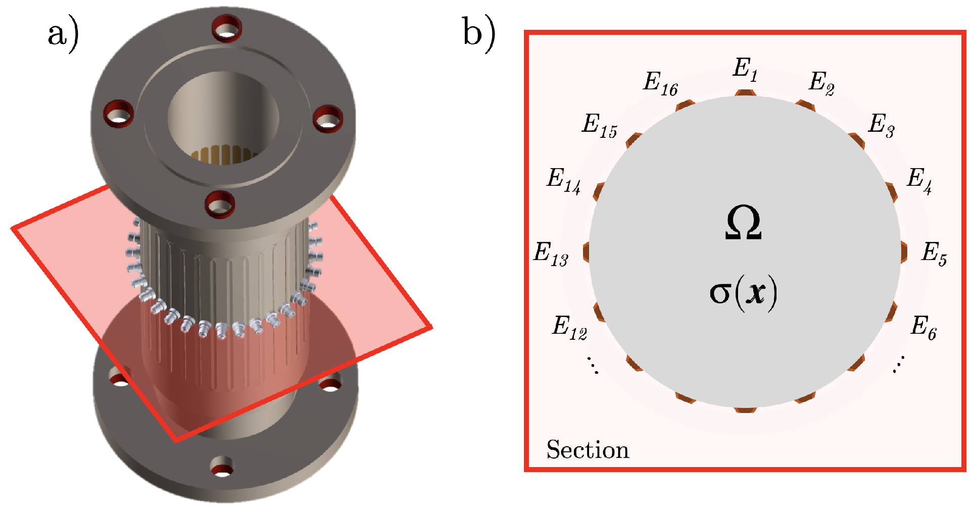
The system
in which the image reconstruction is considered is cylindrical (
Figure 1). EIT is a technique to solve the inverse problem of determining the conductivity function
within the interior of
[
2,
3,
4]. Here,
is the isotropic electrical conductivity field,
the permittivity, and
the angular frequency. EIT operates at
GHz, so the imaginary part of
can be neglected
. The closure of
is denoted as
, and its boundary is
.
In EIT, the conductivity function
is unknown and has to be determined from simultaneous excitations and measurements of the voltage
and the current
, on the boundary. The Maxwell equations define
to be divergence free. Thus, Ohm’s law gives the partial differential equation:
The EIT detector contains a set of
electrodes. On each electrode
for
(
Figure 1b), the potential
and the current
are either given or measured, defining the boundary conditions. Equation (
1) is taken with either the
Dirichlet boundary conditions:
or the
Neumann boundary conditions:
where
is the unitary vector on the surface pointing outward at
. The Neumann boundary conditions have the additional requirement that:
as required by Equation (
1) for well-posedness. In addition, in the case of imposed potentials, the Dirichlet boundary conditions are chosen with the average-free boundary voltage requirement:
in order to define the ground value.
The so-called Dirichlet-to-Neumann (DtN) map
is the operator that links the imposed potential (i.e., Equation (
2)) to the current on the boundary. Equivalently, the Neumann-to-Dirichlet (NdD) map
yields the voltage distribution from any given current-density distribution on the boundary (i.e., Equation (
3)). The DtN or NtD map contains the information to determine
from the set of
(or
. The aim of EIT is to reconstruct the conductivity distribution
while
imposing either the
Dirichlet or the
Neumann boundary conditions while
measuring respectively the
currents or the
potentials over the electrodes [
21,
22]. Finally, the measurements relative to different excitation patterns constitute the data frame, which is used to solve the associated inverse problem to reconstruct
.
3. Specifications of the Proposed EIT System
The ONE-SHOT method was introduced in [
17], which contains motivating results that predict the feasibility of the demodulation of simultaneous excitations with respect to their frequencies. Nevertheless, the proof-of-principle experiment is based on a four-electrode EIT system. The number of independent pairs of excitation for such systems is six, implying six simultaneous excitations at six different frequencies. In practical EIT, the number of electrodes is an important parameter since it allows more measurements and a better conditioning of the inverse problem. Usually, EIT systems contain more than eight electrodes.
The need for more simultaneous measurements is the motivation to evolve the ONE-SHOT method with the increased number of electrodes and, consequently, the number of excitation frequencies. This section discusses the choice of developing the ONE-SHOT excitation strategy for 16 electrodes in
Section 3.1. Secondly, the ONE-SHOT excitation strategy is generalized to any number of electrodes in
Section 3.2 and then adapted for 16 electrodes in
Section 3.3. This process increases significantly the number of independent pairs and the complexity of the corresponding excitation patterns. Finally, choosing the frequencies is a challenging task. A choice is proposed in
Section 3.4 to ensure discriminability, a high rate, and adaptivity to high-speed hardware systems.
3.1. Adequate Number of Electrodes
A large number of measurements is required to well condition the inverse problem for an accurate and stable solution. Consider an EIT device containing a set of
electrodes. The maximum number of measurements is:
where
N is the total number of independent excitation pairs, i.e.:
As , the dataset size increases rapidly as the number of electrodes increases. One can expect that larger values of the parameter lead to images of better quality.
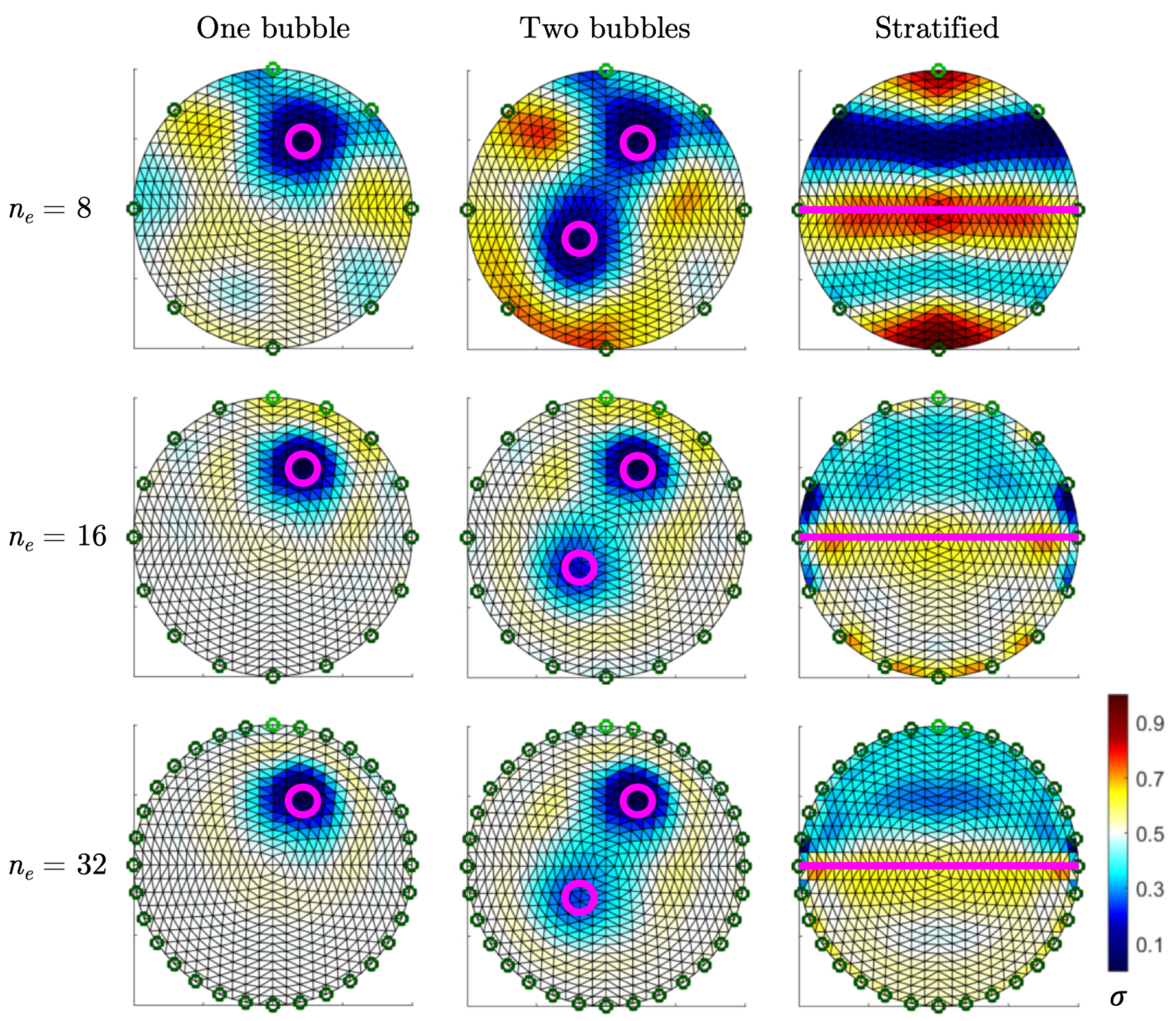
To evaluate this, the open access code EIDORS (Electrical Impedance Tomography and Diffuse Optical Tomography Reconstruction Software) [
23] was used. The code provides software algorithms for forward and inverse modeling for EIT and diffusion-based optical tomography, in medical and industrial settings. Synthetic data of several flow patterns with EIT detectors containing
8, 16, and 32 electrodes are computed. The data are associated with an image based on the linear back projection reconstruction algorithm. This non-iterative method projects the set of voltage variations
between homogenous and an inhomogeneous conductivity data onto the maps of conductivity change
with a set of sensitivity coefficients
S calculated with a linearized version of the inverse problem [
24].
In the simulations of
Figure 2, the domain is filled with homogenous water of conductivity 0.5 S·m
−1 with the addition of steam bubbles of conductivity
S·m
−1. Three patterns are represented in the figure. The number of measurements is
for
,
for
, and
for
. For every pattern, increasing
improves the image quality, as expected. However, the situation
does not give much more accuracy than
, even if the number of measurements is multiplied by more than eight. This result is a known matter in the field of EIT.
Any system with a high frame rate brings an important amount of data. The balance between high image accuracy and low data size led us to develop an EIT system with a specific number of 16 electrodes. According to Equation (
7), the full set of excitations for an EIT system of 16 electrodes is
.
3.2. General Simultaneous Excitation Pattern for Electrodes
ONE-SHOT has to be adapted for a larger number of electrodes. As in Equation (
7), the total number of independent measurements
N defines the number of frequencies that have to be generated simultaneously to maximize the number of measurements for a given system. The excitation is a set of voltages imposed on the electrodes and is generated from a basis of
N sines. Moreover, as discussed in
Section 2 the excitation pattern ensures that the sum of boundary voltages is zero at any time.
One defines the signal
as:
Then, given an arbitrary number
of electrodes, one defines the excitation voltage
at an arbitrary electrode
using the following recurrence relation:
where:
and with
designating the
element of the identity defining the voltage
, under the convention that the terms
are always ordered with increasing index
i in such an identity. Moreover, in (
9), we adopt the convention that a sum is identically zero if the value of the starting index is larger than that of the ending one.
3.3. Simultaneous Excitation Pattern for 16 Electrodes
We are now interested in applying Equation (
9) in the situation of
electrodes. In this situation,
and the set of excitation voltages
is:
where the frequency
is the
frequency for
. Finally, the verification of Equation (
5) from the excitation pattern of Equation (
11) is straightforward.
3.4. Determination of the Excitation Frequencies Based on the Measurement Time Window
The main advantage in the use of a continuous multi-frequency excitation method is the absence of transients between successive projections, resulting in a diminution of the measurement error from the absence of the residual voltage in the electrode–electrolyte contact impedance. Concerning ONE-SHOT, the values of the frequencies remain as free parameters. In this section, we suggest suitable values based on the performances of the DAQ system.
The first observation is that in order to ensure continuous excitations and measurements in parallel, the frequencies of the excitation signals have to be harmonics of a fundamental frequency
. A wise choice is to define
as the frequency of the Discrete Fourier Transform (DFT) of a
P-point measurement sequence
and
p the discrete time. The discretisation of the time is due to the sampling rate of the DAQ system at the frequency
, with the discretisation time interval
, implying:
The DFT of the real-valued sequence
in the
measurement channel is:
with
, and a synchronous sampling is assumed. The real and imaginary parts of
:
and:
define the module
and the phase
of each frequency domain sample
:
and:
The adequate situation where the frequencies
of the generated sines
are multiples of
leads to the following observation: To each
k-coefficient is associated a frequency
, which is linked to the DFT computation frequency
by
, for
, and the following difference, which defines the resolution in the Fourier space:
Choosing the generated frequencies as harmonics of leads to a match between and such that , for and .
This observation is particularly interesting as with a given magnitude is associated a frequency , which corresponds to one and only one generated signal frequency on the electrode n. Therefore, the set of for all n and k is one frame of the EIT data. The frame is acquired at the frequency and contains the full set of independent excitations and measurements to define the Dirichlet or the Neumann boundary conditions.
A first remark is that the highest frequency
is constrained below the Nyquist limit:
. A second remark concerns the phase shift, which describes the difference in radians when two or more alternating quantities reach their maximum or zero values. The phase shift of an electric signal passing through a material depends on the frequency [
16]. In ONE-SHOT, the continuous generation of signals makes the phase shift independent of the Fourier magnitude. This is true because of the choice of the generated signals that are harmonics of the Fourier computation time window.
In standard EIT, the measurement associated with one excitation configuration corresponds to a voltage or current input over one or several periods of an alternative excitation at a given fixed frequency. The corresponding data are a set of tens of points per measurement, which multiplied by
M (Equation (
6)) gives the total number of samples per frame. On the other hand, in the Fourier space, the corresponding data for the same measurement becomes a single element
with
n and
k defined. Building a data frame with the Fourier elements reduces significantly the data size.
Finally, the determination of the frequencies for the application of a 16-electrode ONE-SHOT excitation strategy strongly depends on the acquisition rate of the DAQ system and the choice for the number of measurement points P used to compute the DFT.
6. Preliminary Experimental Results with 15 Different Frequencies
As discussed in the Introduction, the imaging rate of the well-established X-ray tomography suddenly increased when considering several pairs of emitters and receptors for simultaneous measurements. The novel idea, which consists of applying simultaneous excitations and measurements in EIT, brings new challenges due to the fundamental differences existing between such hard field and soft field systems. Apart from the radical difference in solving the inverse problem (
Section 2), multifrequency excitations and measurements have to be considered with the association of TDM in the ONE-SHOT strategy.
The discriminability of the raw data is discussed in
Section 6.1 in two harmonic ranges. In
Section 6.2, the noise measurement is shown with a discussion of the SNR of the measured data.
Section 6.3 introduces the images reconstructed from a set of measurement data.
6.1. Raw Data
The ONE-SHOT excitation strategy has as its goal one single excitation for all independent pairs of electrodes, resulting in the generation of 240 positive and negatives sines (Equation (
11)) of 120 different frequencies (Equation (
7)) for 16 electrodes. Implementing ONE-SHOT is a challenging task as it requires fast voltage excitations of arbitrary signals and FFT computation of current measurements, all in parallel over numerous channels. Nevertheless, the simulation results in
Section 5 are a great incentive to build the experiment as described in
Section 4.
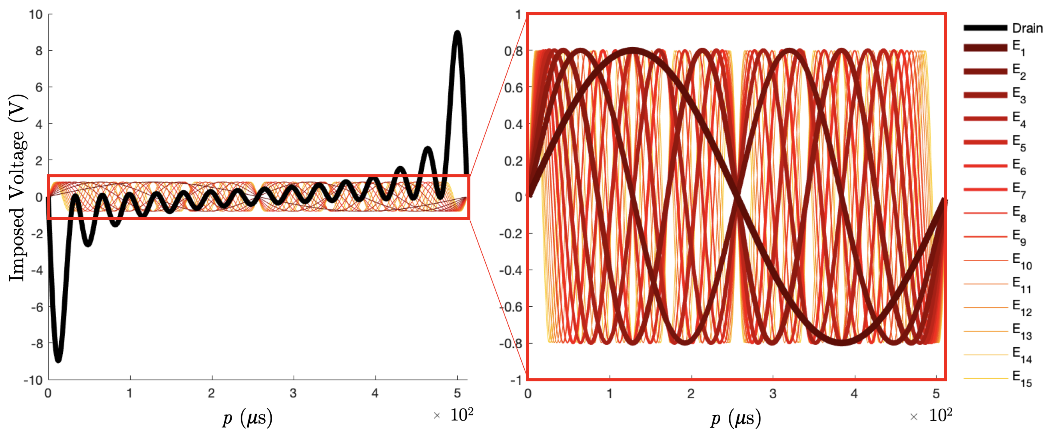
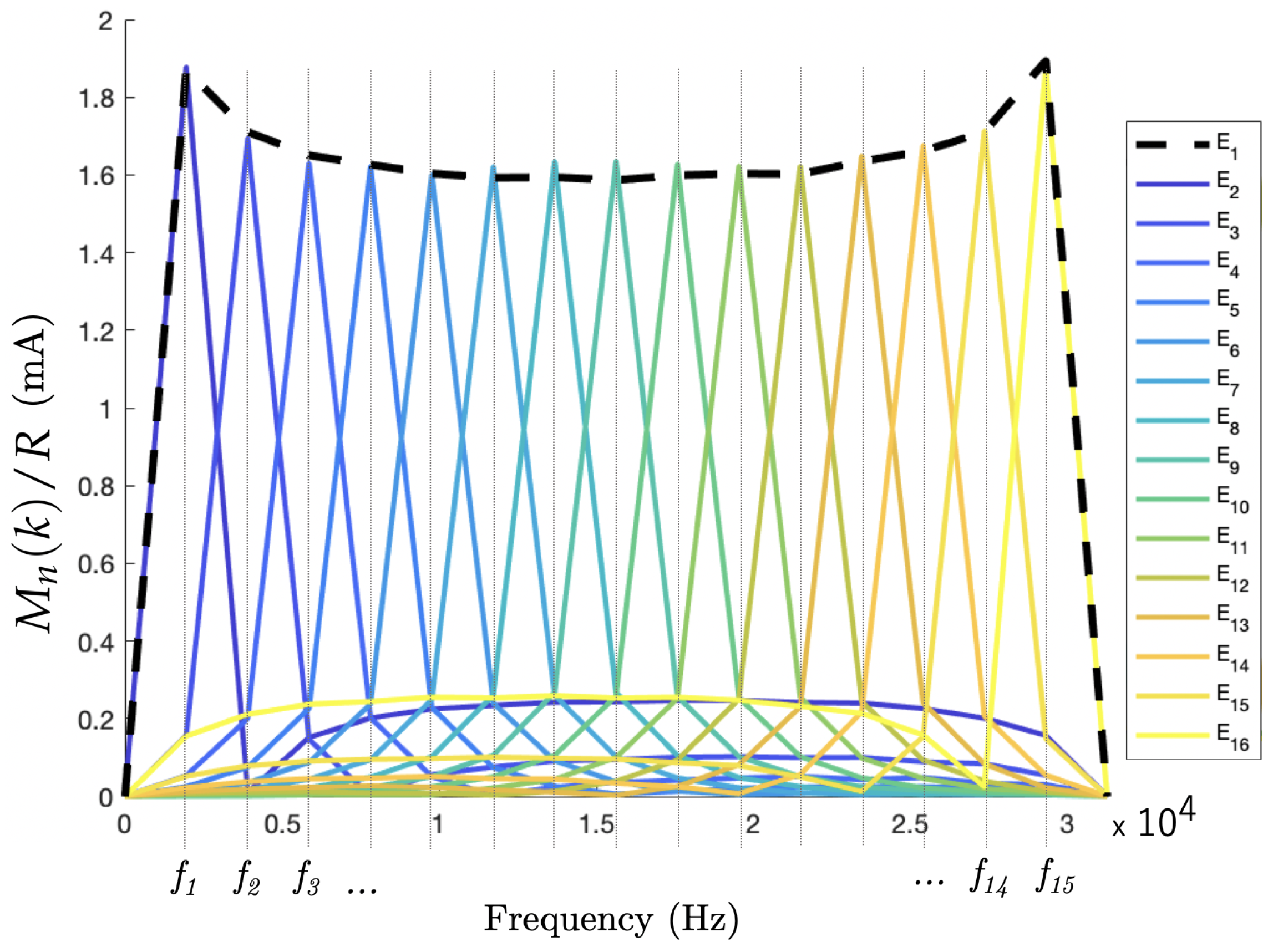
The preliminary results in this experiment are presented to prove the feasibility of using TDM in EIT, based on the simultaneous excitation of 30 positive and negative sines at 15 frequencies and the experimental DFT reconstruction of the same voltage excitation pattern as in
Figure 4. Two frequency domains are investigated: the low harmonic range where the 15 positives sines are the 15 first harmonics of the DFT frequency
(
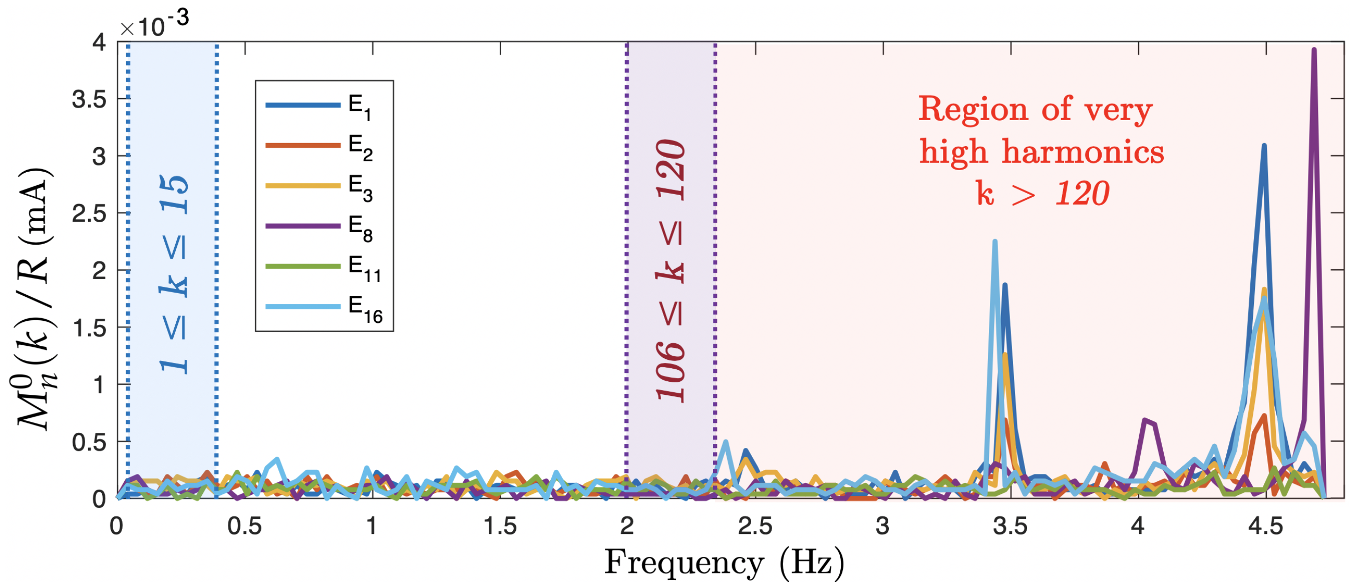
Section 3.4). Furthermore, the high harmonic range contains the harmonics 106–120: as discussed above, these higher frequencies are planned to be generated in the future development of a full simultaneous excitation set.
6.1.1. Experimental Results in the Low Harmonic Range
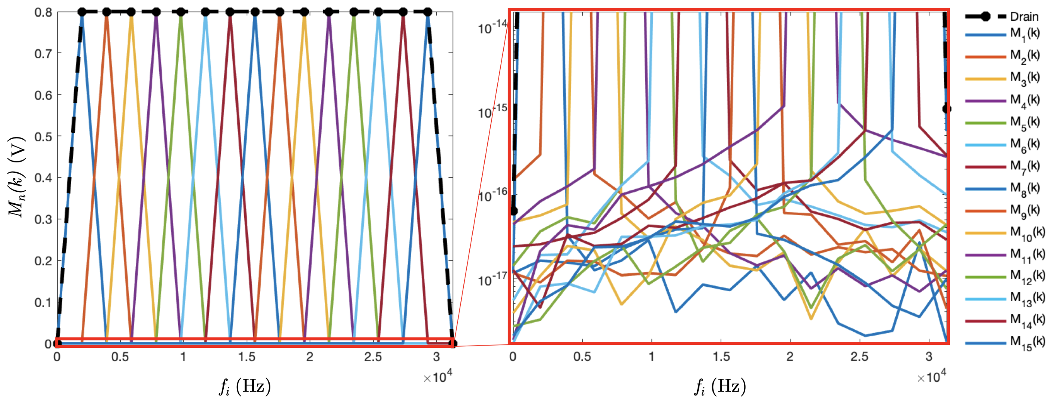
An experiment was set up to measure a homogenous field of conductivity 300 µS/cm. The results in the low harmonic range (
Figure 7) are the DFT magnitudes
of the 16 experimental measurement signals computed from
data points, at a frequency of 1953.125 Hz for a data sampling of 1 MS/s. The results are shown as the current by including
, the resistance in the measurement channel on the PCB. The authors observed a good accordance with the simulations of
Section 5. The comparison of the experimental results (
Figure 7) with the simulated DFT reconstruction of pure sines (
Figure 4) led to the following observations:
The readers familiar with EIT may expect the following phenomenon. In the experimental data, at the bottom of
Figure 7 and
Figure 8, non zero currents were measured over electrodes that were not excited at the corresponding frequency. Let us consider an electrode
with
excited by a single sine of frequency
. In the Fourier space (
Figure 7 and
Figure 8), the measured current passing through an electrode gives non-zero values for other frequencies. The reason comes from the electric potential difference that appears between the excited electrode
with an imposed potential
with
and a non-excited electrode
whose potential is
for a given frequency
in the Fourier space (
Figure 5). This effect is particularly large for the current in the adjacent measurement of the drain electrode in
and
. These data depend on the electrical conductivity distribution inside the body and have to be considered as well.
The magnitudes of the Fourier coefficients in the experimental results were lower for the mid-range harmonics than
and
: Considering the finite electrical conductivity inside the system, the current resulting from the potential imposed between two neighboring electrodes was larger than the current resulting from the same potential imposed between two opposite electrodes in the circular shape of the EIT sensor [
16].
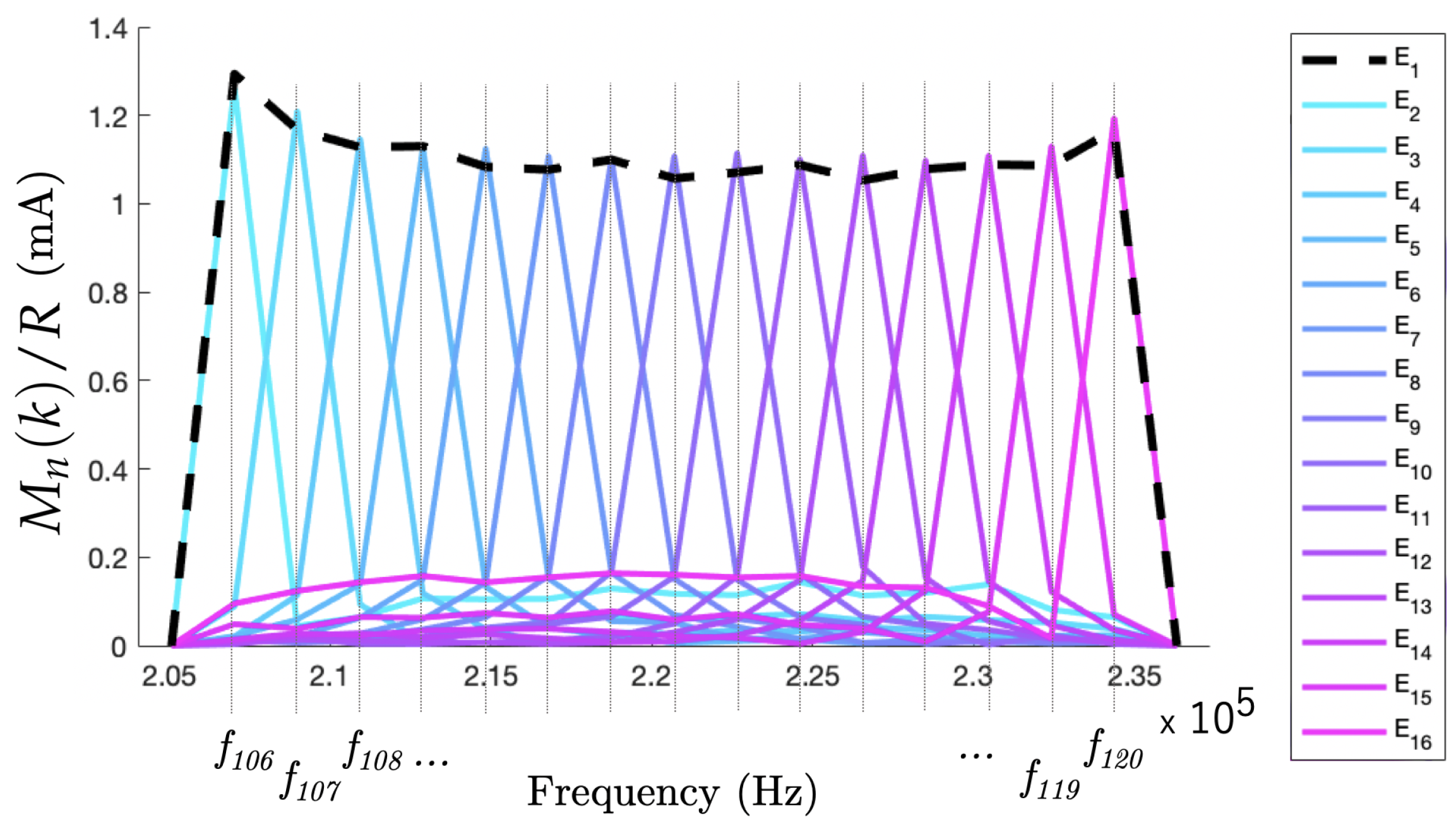
6.1.2. Experimental Results in the High Harmonic Range
The main prospect of the ONE-SHOT excitation strategy is to consider simultaneous excitations at 120 different frequencies for the EIT sensor of 16 electrodes. As in
Section 3.4, the frequencies were chosen to be harmonics of the fundamental frequency
. The 120th harmonic
was then 234.357 kHz. We investigated the performance of ONE-SHOT in this higher harmonic range.
The experimental measurement resulted in the high harmonic range from
–
is shown in
Figure 8. The discrimination of the signals by frequency offered equivalent performances to the low harmonic case. However, an important remark is that the signal amplitudes in the high harmonic range were lower than previously due to the impedance of water, which depends on the excitation frequency. The result was a weaker response in amplitude in the high harmonic range for the same conductivity change in the system. Investigations are ongoing for calibrating the amplitude of the generated sines to have a similar response in every harmonic for a future generation of a full set of 120 excitations.
6.2. Noise Measurement
A set of voltage magnitudes
, defined as in Equation (
16), was experimentally measured without any excitation to identify the noise spectrum. The results in
Figure 9 show localized peaks in the noise amplitude beyond the high harmonic frequency domain.
The SNR of a signal measured at a given electrode
n and tagged with a given frequency
k is defined as follows:
where
is the number of data taken for averaging. The noise in the low harmonic range resulted in an SNR of the raw signal of 69.1 dB in the lowest frequency magnitude in the excitation electrode channels when averaging the signal from
samples. In a non-excited channel, the signal was O(0.1) weaker, resulting in an SNR of about 60 dB depending on the signal magnitude. In the high harmonic range, the SNR was 59.6 dB for the highest harmonic.
The very high frequencies
kHz, bounded above by the Nyquist limit, could be considered as excitation frequencies. However, a proper shielding of the DAQ system must be investigated. A large part of the noise was caused by electrical noise in the PCB. For this reason, a new PCB is being manufactured. Finally, the results showed that the noise completely covered the DFT systematic uncertainty (
Section 5.1), which is completely negligible.
6.3. Image Reconstruction from 16 Datasets
The main objective of the present manuscript is the implementation of a method to obtain a very fast EIT data frame acquisition rate. From such data, the user can then reconstruct an image with any given reconstruction algorithm in post-processing, a step that we consider to be distinct from our main goal. As an example, we are interested in the image reconstruction of the above data. However, the datasets are incomplete by comparison with the ONE-SHOT excitation prospects of Equation (
11). A solution consists of reconstructing the full dataset in the post-processing.
The results described above contained a complete set of excitations for the drain electrode. It is possible to consider another drain electrode and another frequency set to obtain another set of measurements, independent of location and frequency.
The rotation of the drain over the 16 electrodes resulted in pairs of excitations. The symmetry suggested to consider only half of the data. The full dataset was deduced and contained the decomposition of 240 signals from 120 excitation pairs, measured over the 16 resistances of the PCB. Therefore, the full dataset included a total of 1920 elements. To sum up, the sequential excitations with the drain located on each of the 16 electrodes resulted in a dataset equivalent to the one expected by the full implementation of the ONE-SHOT method.
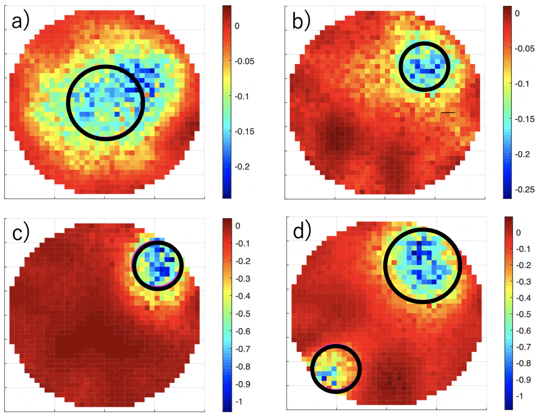
Several datasets were measured from the inclusion of non-conducting PMMA rods in the test section of
Figure 1 filled with tap water with a conductivity of
= 635 µS·m
−1. The one-step least-squares iterative reconstruction method [
27,
28] was implemented, and the results are shown in
Figure 10.
The results showed similar image reconstruction performances as another EIT system [
16] based on TDM and using the same reconstruction algorithm. As usual in EIT, the sensitivity was much higher close to the electrodes. This effect resulted in sharp gradients when imaging the inclusions inserted at the edge.
Finally, the frame rate of the ONE-SHOT system can be changed by integrating the FFT over more or less data points. For instance, choosing the FFT to be computed over 512 points as considered in this article resulted in the frame rate of 1953 fps. In this case, the 120 frequencies can fill all the discrete values from 1953 Hz to the Nyquist limit of 500 kHz with µs = 1953 Hz the minimal gap between two neighboring values. The high frame rate was at the cost of a large frequency bandwidth.
7. Conclusions
This article assessed the feasibility of simultaneous excitations and measurements using a multi-frequency strategy for high-speed electrical impedance tomography, based on the ONE-SHOT excitation method. The motivations for increasing the data frame rate for EIT measurement followed by an overview of the mathematical aspect of EIT were presented in
Section 1 and
Section 2, respectively. The requirements for the hardware system based on the excitation strategy and measurement process, as well as the motivations to determine the number of electrodes were discussed in
Section 3. An efficient hardware solution for implementing the simultaneous EIT excitation strategy was proposed in
Section 4 with an analysis of the error and noise propagation through the measurement process in
Section 5. Finally, experimental results were shown in
Section 6 in the low and high harmonic ranges of the excitation signals.
Table 1 compares the performances of ONE-SHOT with a number of existing high-rate EIT systems. The description of the different hardware systems contains several characteristics that have to be considered while comparing the data frame rates, including the Number of Measurements per Seconds (NMS). Firstly, the AI sampling frequency directly impacted the data frame rate. Secondly, the data size was an important factor to maximize for a good conditioning of the inverse problem. Thirdly, the noise also directly impacted the image quality. The noise of the ONE-SHOT system was the value currently measured in a partially-shielded DAQ prototype. Future tests, especially including the new PCB, will result in better performances in terms of SNR.
The next experimental step is to measure a full scan by exciting all independent pairs of electrodes. For a 16-electrode EIT device, the number of frequencies becomes 120, bringing several new challenges. Mainly, the limit imposed by the Nyquist frequency of 500 kHz for the current system associated with the resolution in the frequency space from the choice of the DFT computation time window results in a maximum number of harmonics. Adding more frequencies may impose a longer time window, directly impacting the data frame acquisition rate. However, considering frequencies in the very high harmonic range may drastically affect the SNR due to higher resistivity and noise peaks. Furthermore, the limited physical space in the FPGA restricts the number of sine generators. The prospects of the performances of ONE-SHOT are also shown in
Table 1. In these prospects, the DFT computed over measurements of
points may increase the data acquisition rate, keeping
kHz, below the Nyquist limit.

 ,
, 


