On Optimal Imaging Angles in Multi-Angle Ocean Sun Glitter Remote-Sensing Platforms to Observe Sea Surface Roughness

 ,
,
Abstract
:1. Introduction
2. Materials and Methods
2.1. Estimation Model for Sea Surface Roughness (SSR)
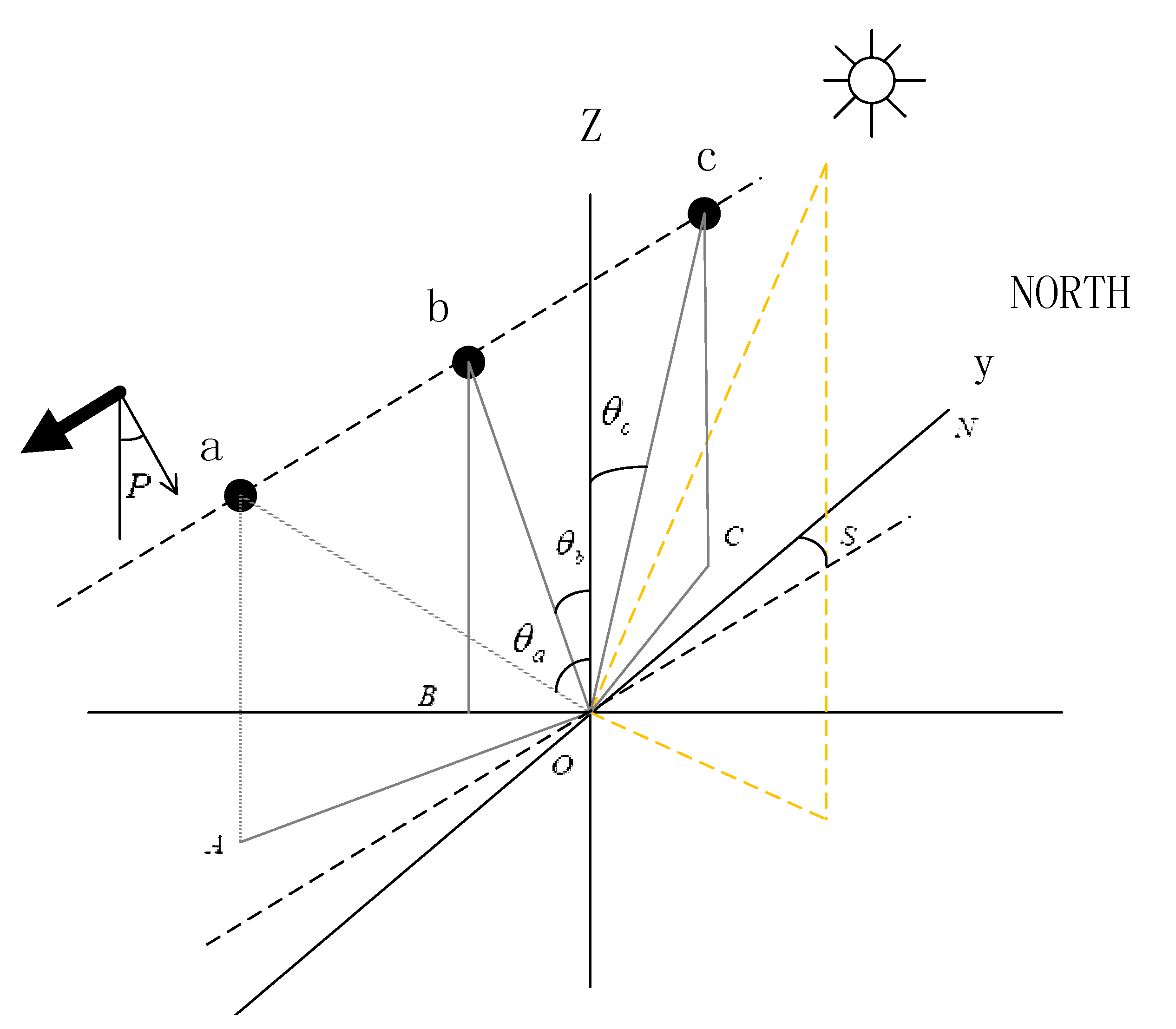
2.2. Sun Glitter (SG) Geometry in Stereo Images
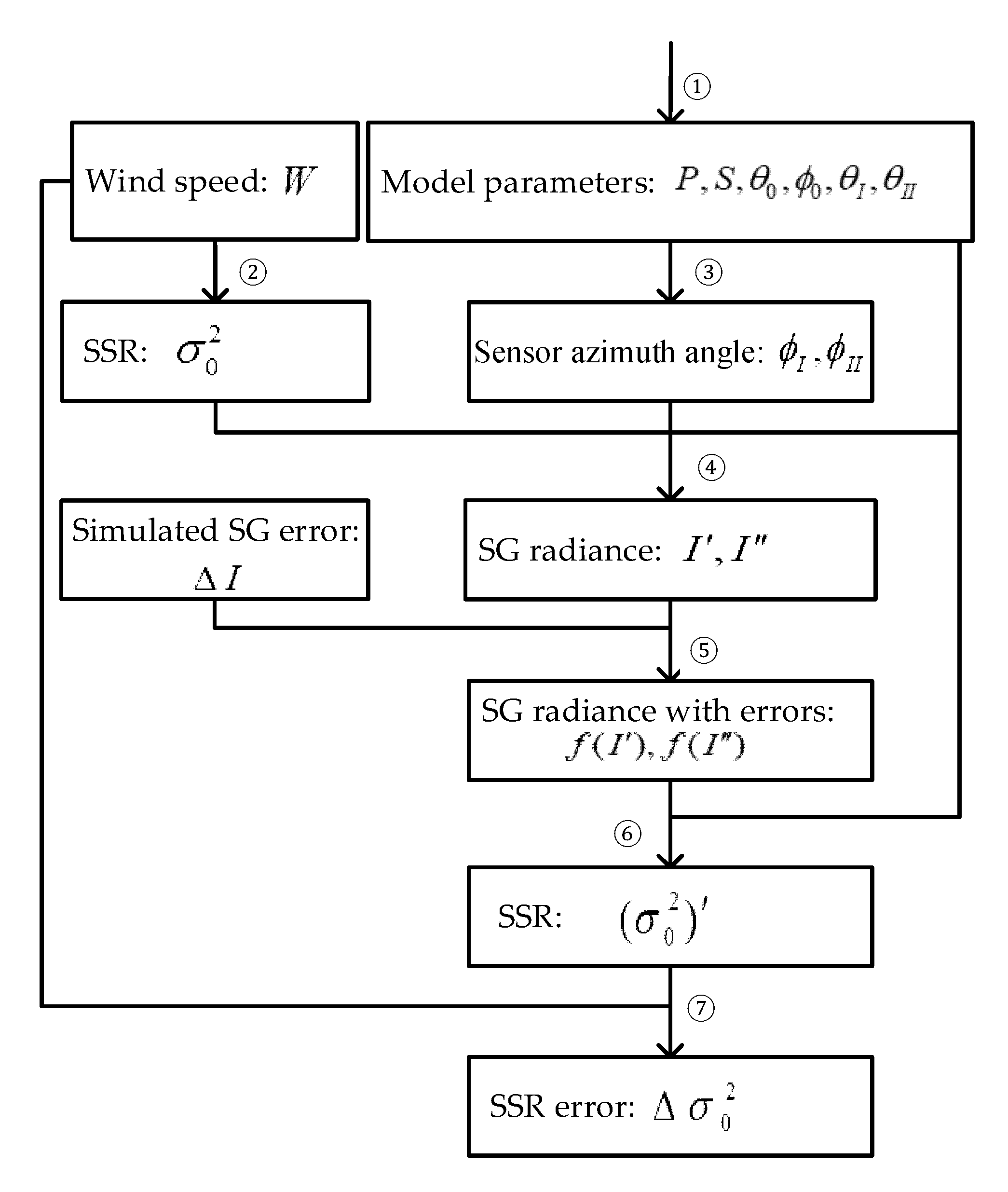
2.3. Simulation Model
- ①
- Input model parameters and determine sensor pointing angle (P), scene orientation angle (S), sun zenith angle (), sun azimuth angle (), and SVA combination (,);
- ②
- Input the sea surface wind speed (W), use the CM model [1] to calculate SSR attributable to sea surface wind (), and use the SSR as the real value of the assessment;
- ③
- Combine the sensor information input in ①, calculate sensor azimuth angles (,) under SVA combinations (,) according to Equations (14), (15), (17) and (18);
- ④
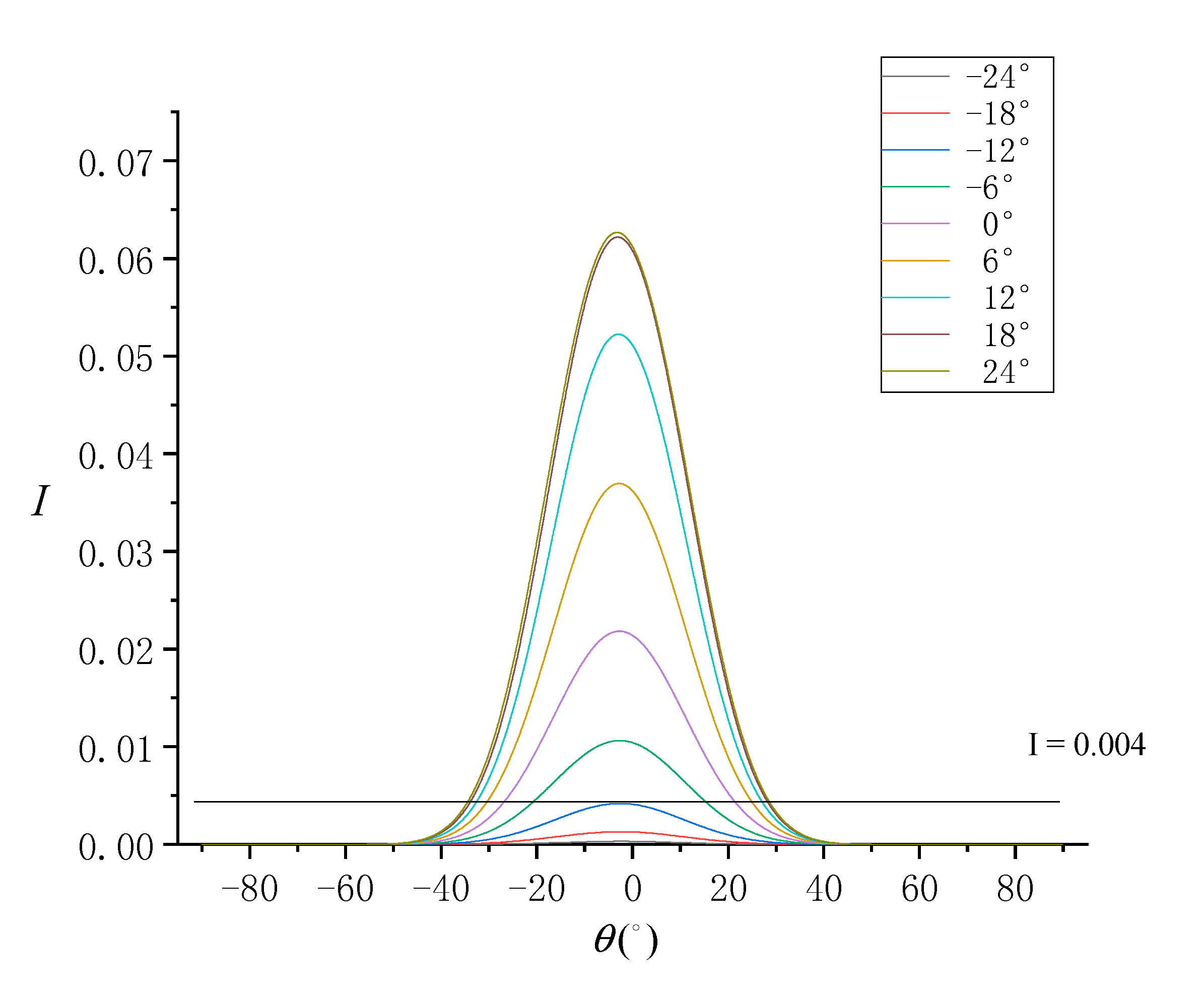
- Simulate a pair of normalized SG radiance (, ) (Equation (9));
- ⑤
- Add the simulated error () to the normalized SG radiance (, ). Here, we use a 5% multiplicative error and an additive error of 0.00005 according to the signal-to-noise ratio of the ocean optical remote sensor and the general radiation correction error (), and get a pair of normalized SG radiance with errors (, ).
- ⑥
- Apply , and related parameters to the SSR estimation model based on multi-angle SG (Equation (12)). Then get the estimated SSR ()’);
- ⑦
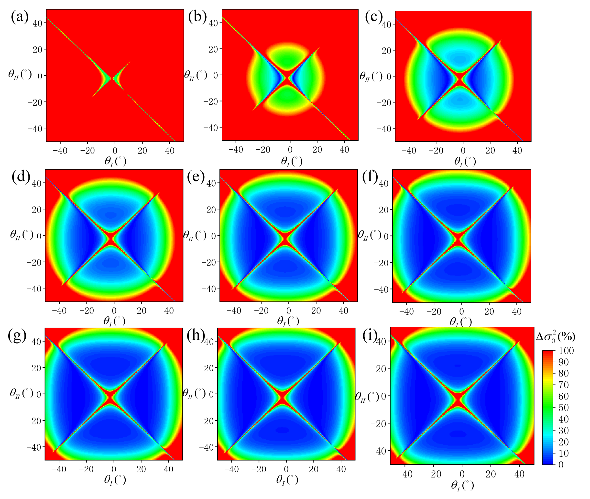
- Calculate the error () between the estimated SSR ()’) and the real SSR () attributable to wind speed.
3. Simulation and Analysis
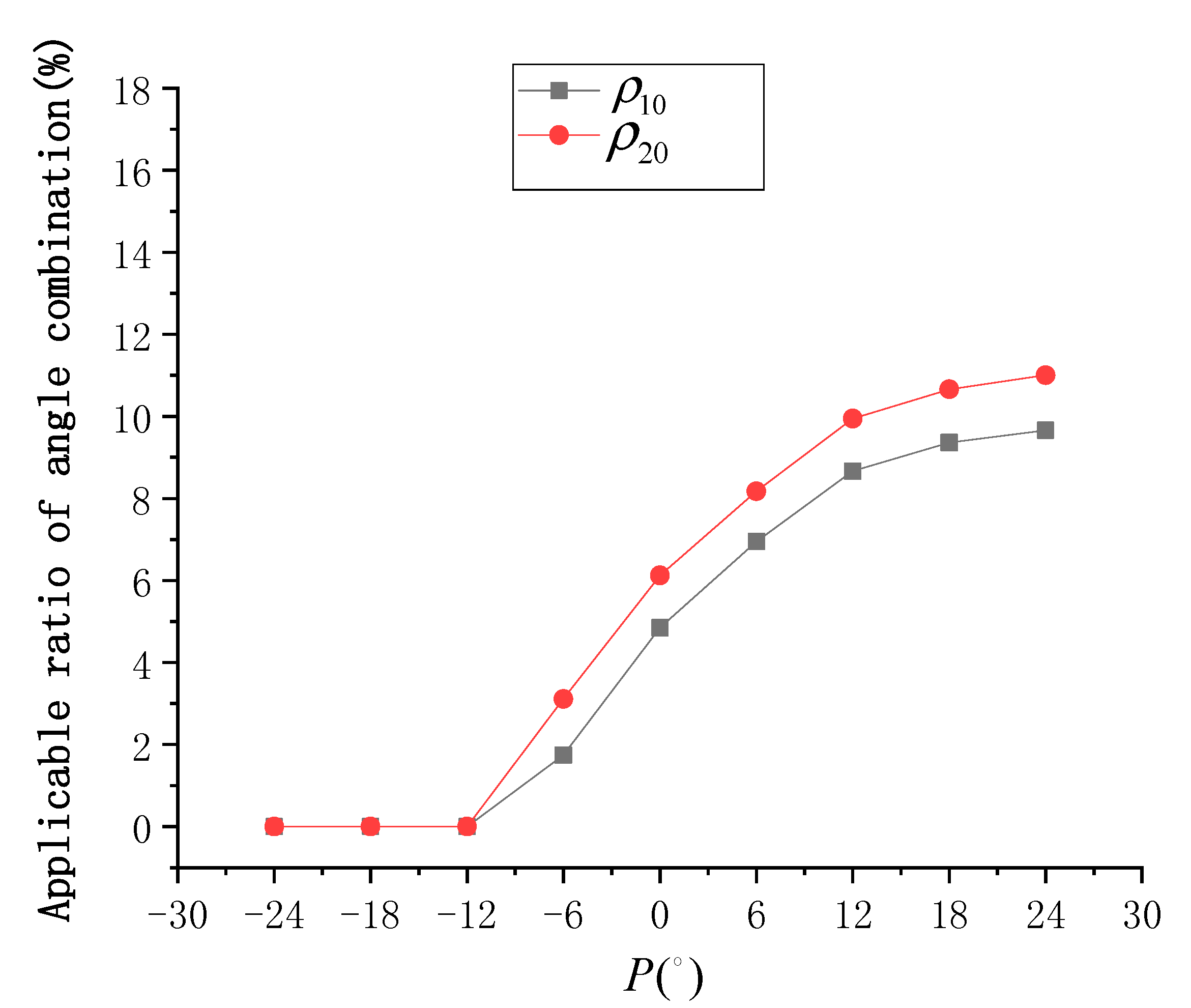
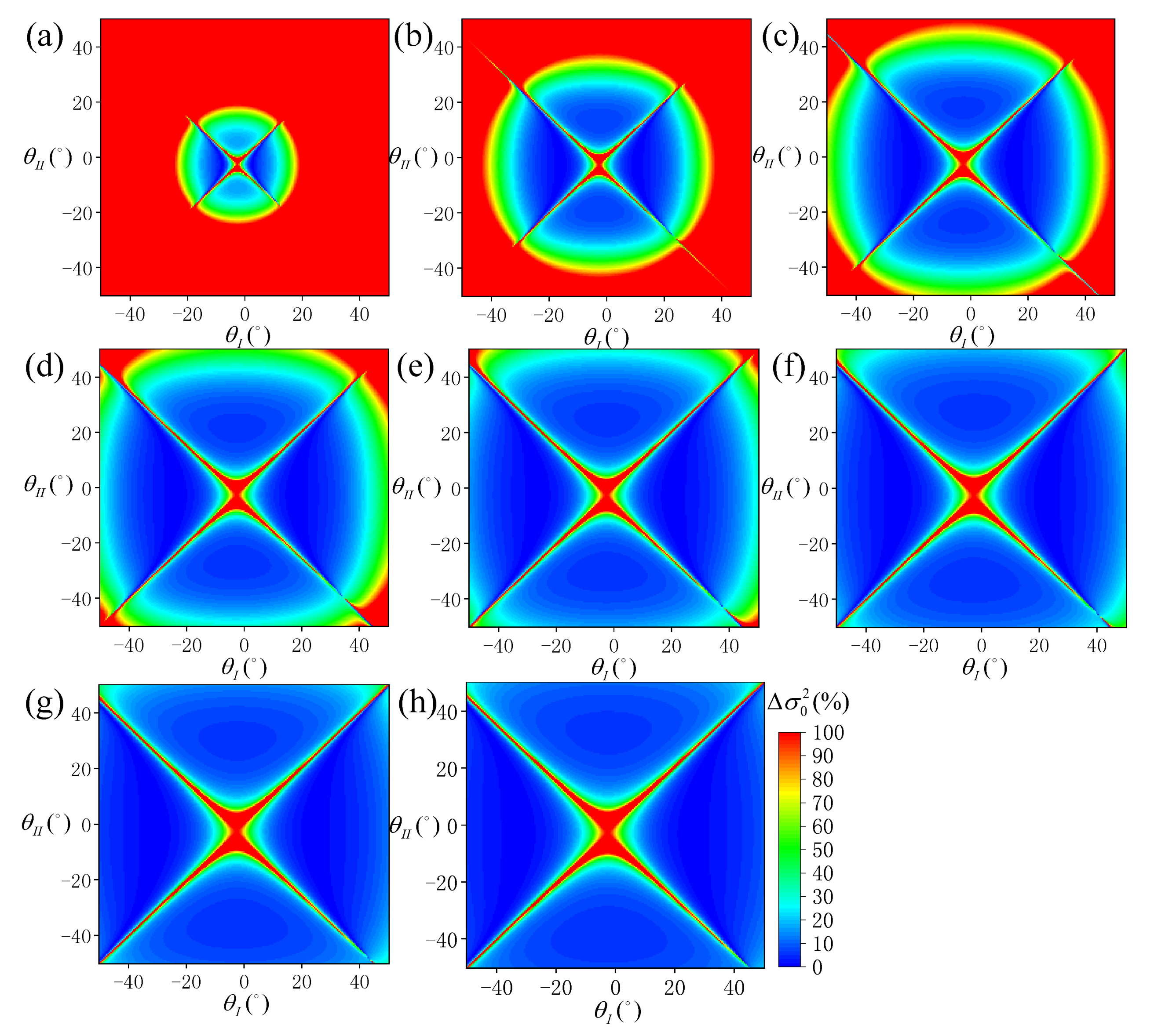
3.1. Pointing Angle
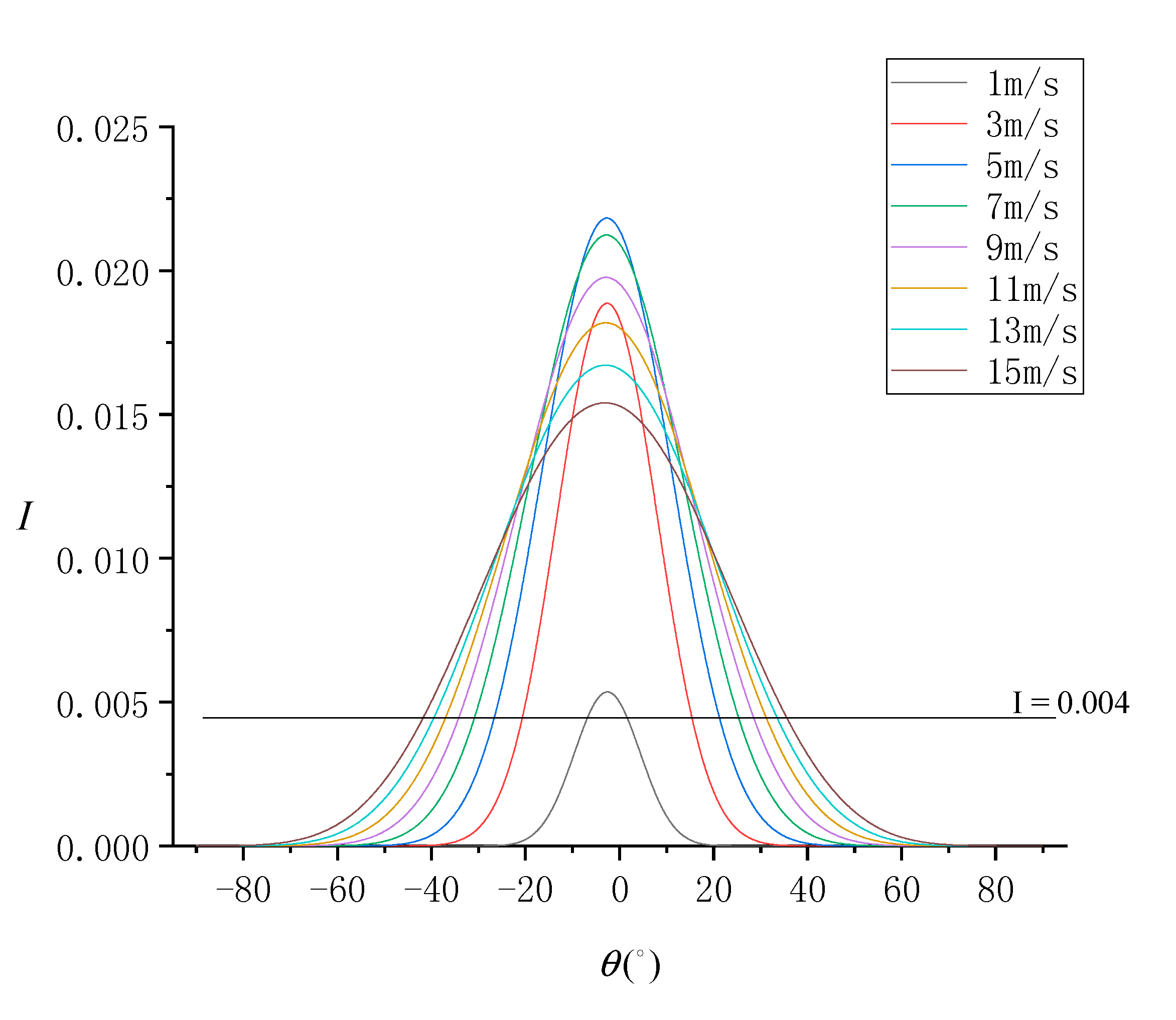
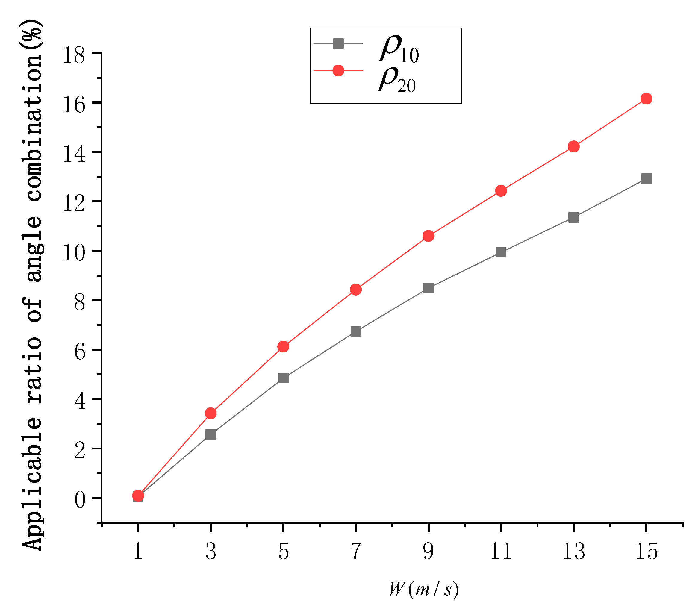
3.2. Wind Speed
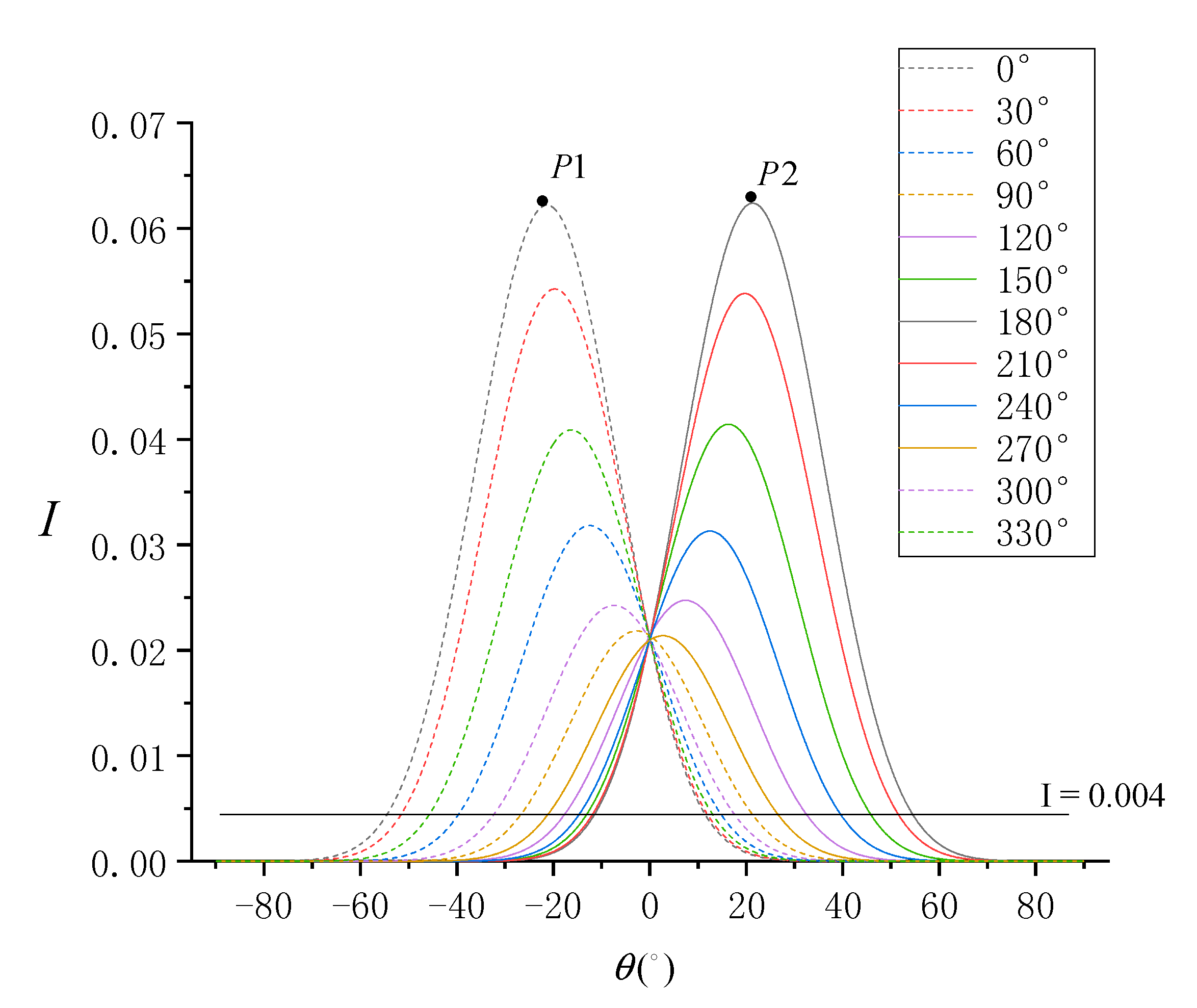
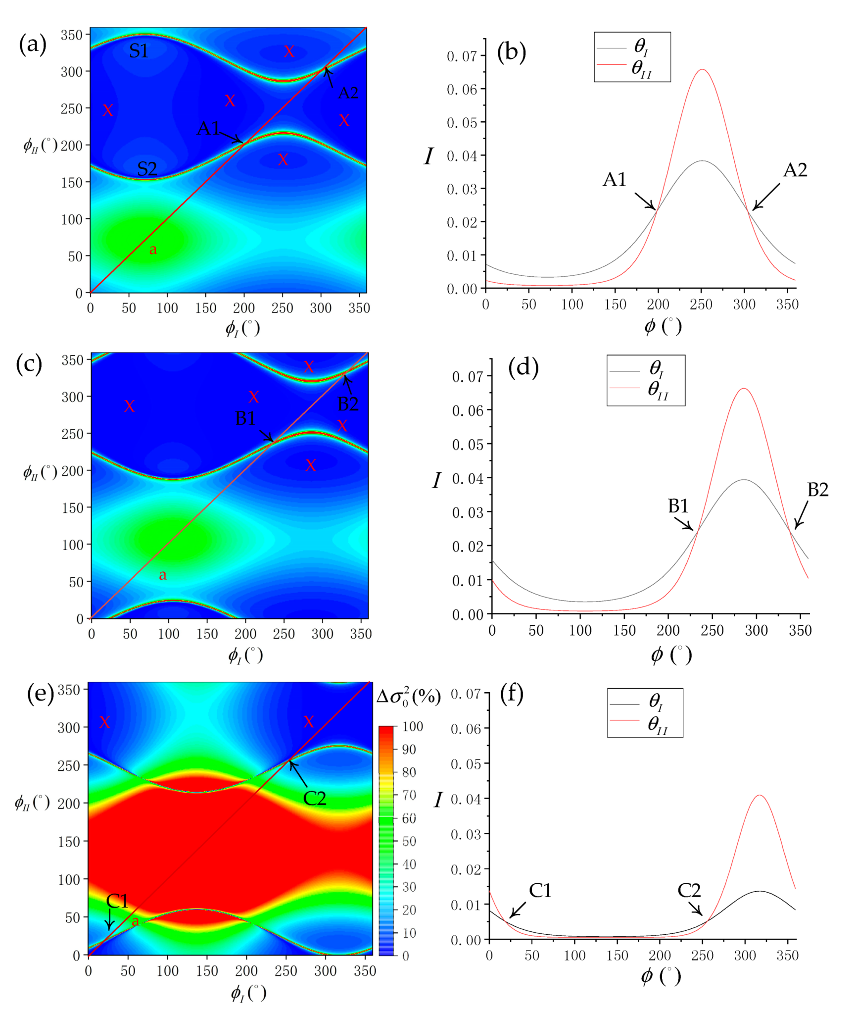
3.3. Sun Azimuth Angle
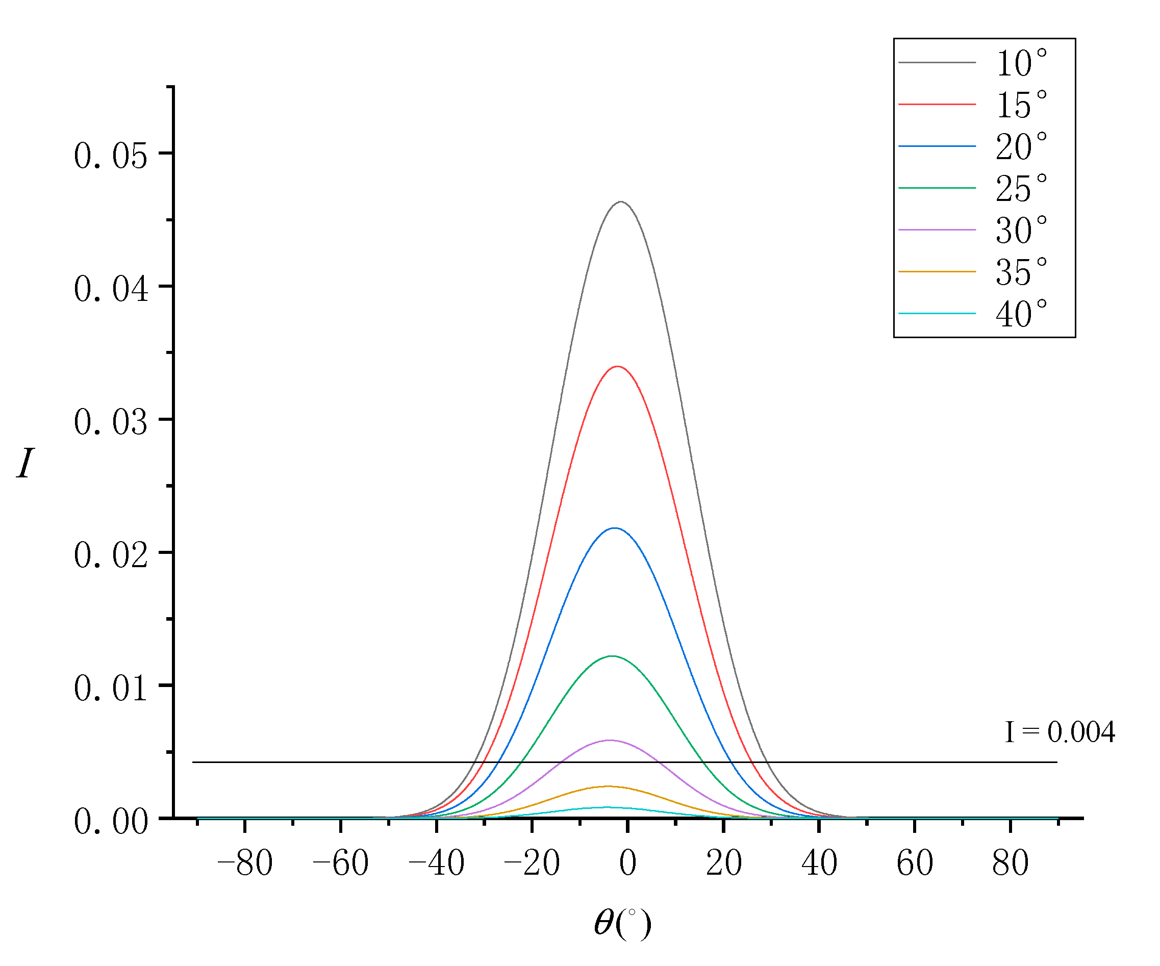
3.4. Sun Zenith Angle
4. Discussion
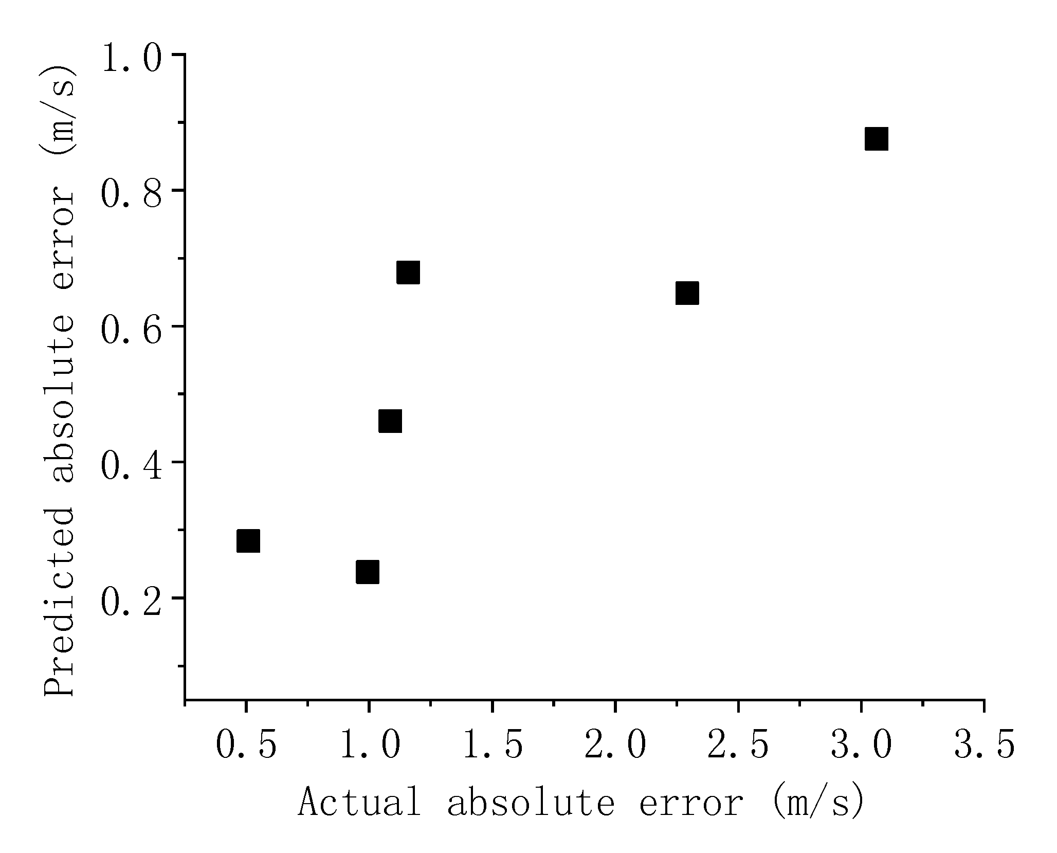
4.1. Comparison of Predicted and Actual Error
4.2. Optimal Relative Azimuth Angles in the Multi-Angle Remote-Sensing Platform
5. Conclusions
Author Contributions
Funding
Acknowledgments
Conflicts of Interest
References
- Cox, C.; Munk, W. Measurement of the roughness of the sea surface from photographs of the Sun’s glitter. J. Opt. Soc. Am. 1954, 44, 838–850. [Google Scholar] [CrossRef]
- Kay, S.; Hedley, J.; Lavender, S. Sun glint correction of high and low spatial resolution images of aquatic scenes: A review of methods for visible and near-infrared wavelengths. Remote Sens. 2009, 1, 697–730. [Google Scholar] [CrossRef]
- Kay, S.; Hedley, J.; Lavender, S. Sun glint estimation in marine satellite images: A comparison of results from calculation and radiative transfer modeling. Appl. Opt. 2013, 52, 5631–5639. [Google Scholar] [CrossRef]
- Lee, Z.P.; Ahn, Y.H.; Mobley, C.; Arnone, R. Removal of surface-reflected light for the measurement of remote-sensing reflectance from an above-surface platform. Opt. Express. 2010, 18, 26313–26324. [Google Scholar] [CrossRef] [PubMed]
- Gordon, H.R. Atmospheric correction of ocean color imagery in the Earth Observing System era. J. Geophys. Res. 1997, 102, 17081–17106. [Google Scholar] [CrossRef] [Green Version]
- Matthews, J. Stereo observation of lakes and coastal zones using ASTER imagery. Remote Sens. Environ. 2005, 99, 16–30. [Google Scholar] [CrossRef]
- Christian, M.; Kwoh, L.K. Sun glitter in SPOT images and the visibility of oceanic phenomena. Paper Presented at the 22nd Asian Conference on Remote Sensing, Singapore, 5–9 November 2001; pp. 1–6. [Google Scholar]
- Jackson, C.R.; Alpers, W. The role of the critical angle in brightness reversals on sunglint images of the sea surface. J. Geophys. Res. Oceans. 2010, 115, C09019. [Google Scholar] [CrossRef]
- Lu, Y.C.; Sun, S.J.; Zhang, M.W.; Murch, B.; Hu, C.M. Refinement of the critical angle calculation for the contrast reversal of oil slicks under sunglint. J. Geophys. Res. Oceans. 2016, 121, 148–161. [Google Scholar] [CrossRef]
- He, X.K.; Chen, N.H.; Zhang, H.G.; Guan, W.B. The brightness reversal of submarine sand waves in “HJ-1A/B”CCD sun glitter images. Acta Ocea. Sin. 2015, 34, 94–99. [Google Scholar] [CrossRef]
- Yang, K.; Zhang, H.G.; Fu, B.; Zheng, G.; Guan, W.B.; Shi, A.Q.; Li, D.L. Observation of submarine sand waves using ASTER stereo sun glitter imagery. Int. J. Remote Sens. 2015, 36, 17. [Google Scholar] [CrossRef]
- Bréon, F.M.; Henriot, N. Spaceborne observations of ocean glint reflectance and modeling of wave slope distributions. J. Geophys. Res. Oceans. 2006, 111, C06005. [Google Scholar] [CrossRef]
- Chust, G.; Sagarminaga, Y. The multi-angle view of MISR detects oil slicks under sun glitter conditions. Remote Sens. Environ. 2007, 107, 232–239. [Google Scholar] [CrossRef]
- Fox, D.; Gonzalez, E.; Kahn, R.; Martonchik, J. Near-surface wind speed retrieval from space-based, multi-angle imaging of ocean Sun glint patterns. Remote Sens. Environ. 2007, 107, 223–231. [Google Scholar] [CrossRef]
- Matthews, J.P.; Yang, X.D.; Shen, J.; Awaji, T. Structured Sun glitter recorded in an ASTER along-track stereo image of Nam Co Lake (Tibet): An interpretation based on supercritical flow over a lake floor depression. J. Geophys. Res. Oceans. 2008, 113, C01019. [Google Scholar] [CrossRef]
- Harmel, T.; Chami, M. Determination of sea surface wind speed using the polarimetric and multidirectional properties of satellite measurements in visible bands. Geophys. Res. Lett. 2012, 39, L19611. [Google Scholar] [CrossRef]
- Zhang, H.G.; Yang, K.; Lou, X.L.; Li, D.L.; Shi, A.Q.; Fu, B. Bathymetric mapping of submarine sand waves using multi-angle sun glitter imagery: A case of the Taiwan Banks with ASTER stereo imagery. J. Appl. Remote Sens. 2015, 9, 095988-1–095988-13. [Google Scholar] [CrossRef]
- Kudryavtsev, V.; Yurovskaya, M.; Chapron, B.; Collard, F.; Donlon, C. Sun glitter imagery of ocean surface waves. Part 1: Directional spectrum retrieval and validation. J. Geophys. Res. Oceans. 2017, 122, 1369–1383. [Google Scholar] [CrossRef]
- Kudryavtsev, V.; Yurovskaya, M.; Chapron, B.; Collard, F.; Donlon, C. Sun glitter imagery of surface waves. Part 2: Waves transformation on ocean currents. J. Geophys. Res. Oceans. 2017, 122, 1384–1399. [Google Scholar] [CrossRef]
- Zhang, H.G.; Yang, K.; Lou, X.L.; Li, Y.; Zheng, G.; Wang, J.; Wang, X.Z.; Ren, L.; Li, D.L.; Shi, A.Q. Observation of sea surface roughness at a pixel scale using multi-angle sun glitter images acquired by the ASTER sensor. Remote Sens. Environ. 2018, 208, 97–108. [Google Scholar] [CrossRef]
- Lo, M.W. Satellite-constellation design. Comput. Sci. Eng. 2002, 1, 58–67. [Google Scholar] [CrossRef]
- Neckel, H. The solar radiation between 3300 and 12500 Å. Sol. Phys. 1984, 90, 205–258. [Google Scholar] [CrossRef]
- Shao, H.; Li, Y.; Li, L. Sun glitter imaging of submarine sand waves on the Taiwan Banks: Determination of the relaxation rate of short waves. J. Geophys. Res. Oceans. 2011, 116, C06024. [Google Scholar] [CrossRef]
- Gordon, H.R.; Brown, J.W.; Evans, R.H. Exact Rayleigh scattering calculations for use with the Nimbus-7 coastal zone color scanner. Appl. Opt. 1988, 27, 862–871. [Google Scholar] [CrossRef] [PubMed]


| Parameter | Value | Parameter Description |
|---|---|---|
| IFOV | Instantaneous field of view of ASTER | |
| S | 8 (°) | Scene orientation angle |
| h | Satellite height | |
| m | 15 (m) | Image spatial resolution |
| P | 0 (°) | Pointing angle |
| W | 5 (m/s) | Sea surface wind speed |
| 90 (°) | Sun azimuth angle | |
| 20 (°) | Sun zenith angle |
© 2019 by the authors. Licensee MDPI, Basel, Switzerland. This article is an open access article distributed under the terms and conditions of the Creative Commons Attribution (CC BY) license (http://creativecommons.org/licenses/by/4.0/).
Share and Cite
Wang, D.; Zhao, L.; Zhang, H.; Wang, J.; Lou, X.; Chen, P.; Fan, K.; Shi, A.; Li, D. On Optimal Imaging Angles in Multi-Angle Ocean Sun Glitter Remote-Sensing Platforms to Observe Sea Surface Roughness. Sensors 2019, 19, 2268. https://doi.org/10.3390/s19102268
Wang D, Zhao L, Zhang H, Wang J, Lou X, Chen P, Fan K, Shi A, Li D. On Optimal Imaging Angles in Multi-Angle Ocean Sun Glitter Remote-Sensing Platforms to Observe Sea Surface Roughness. Sensors. 2019; 19(10):2268. https://doi.org/10.3390/s19102268
Chicago/Turabian StyleWang, Dazhuang, Liaoying Zhao, Huaguo Zhang, Juan Wang, Xiulin Lou, Peng Chen, Kaiguo Fan, Aiqin Shi, and Dongling Li. 2019. "On Optimal Imaging Angles in Multi-Angle Ocean Sun Glitter Remote-Sensing Platforms to Observe Sea Surface Roughness" Sensors 19, no. 10: 2268. https://doi.org/10.3390/s19102268