Measurement Structures of Image Compressive Sensing for Green Internet of Things (IoT)


School of Computer and Information Technology, Xinyang Normal University, Xinyang 464000, China
*
Author to whom correspondence should be addressed.
Sensors 2019, 19(1), 102; https://doi.org/10.3390/s19010102
Submission received: 7 November 2018
/
Revised: 15 December 2018
/
Accepted: 24 December 2018
/
Published: 29 December 2018
(This article belongs to the Special Issue Green, Energy-Efficient and Sustainable Networks)
Abstract
:Image compressive sensing (CS) is a potential imaging scheme for green internet of things (IoT). To further make CS-based sensor adaptable to low bandwidth and low power, this paper focuses on finding a good measurement structure, i.e., the organization and storage format of CS measurements. Three potential measurement structures are proposed in this paper, respectively raster structure (RA), patch structure, and layer structure (LA). RA stores CS measurements of each column in an image, and PA packets CS measurements of overlapping patches forming an image. LA enables the measuring of small blocks and recovery of large blocks. All of the three structures avoid high computation complexity and huge memory in the process of measuring and recovery, and efficiently suppress the annoying blocking artifacts which often occur in traditional block structures. Experimental results show that RA, PA, and LA can efficiently reduce blocking artifacts, and produce comforting visual qualities. LA, especially, presents both good time-distortion and rate-distortion performance. By this paper, it is proved that LA is a suitable measurement structure for green IoT.
1. Introduction
1.1. Motivation and Objective
Up to this day, compressive sensing (CS) [1,2] has already become a commonplace technology, and it is widely used in imaging applications to sample various signals, e.g., magnetic resonance imaging (MRI) [3], multispectral imaging [4], synthetic aperture radar (SAR) imaging [5], etc. Moreover, in the field of microwave tomography and antenna synthesis, CS also becomes a popular tool, e.g., [6,7] use CS to solve the non-linear inverse scattering problems, and [8,9] use CS to solve power synthesis of maximally-sparse arrays. These applications reflect the low cost of CS in capturing invisible light which brings a cheap and portable sensor. Many researchers recognize that CS is an energy-efficient sampling method which provides a good imaging quality at the same time, so they have turned their attention to the application of CS to green internet of things (green IoT) [10,11].
To achieve green IoT, some frameworks [12,13,14] of image CS are reviewed and newly developed to meet the demand for these energy-hungry devices. These works focus on how to design sampling and recovery algorithms to get better imaging quality in low-rate and low-power cases, but they have not considered how to organize and store CS measurements to improve the efficiency of sensors in performing CS. In green IoT, measurement structure, i.e., the organization and storage format of CS measurements, is important for sensors to produce a compact bitstream that could reduce the energy consumption of transmission. Therefore, the objective of this paper is to find a good measurement structure to make CS-based sensors energy-efficient.
1.2. Related Work
In existing works, two kinds of measurement structures are used to organize CS measurements, i.e., whole structure (WH) and block structure (BL). WH regards whole image as a column vector, and measures it by using a random matrix. The early works [15,16,17,18] on image CS extensively applied WH in CS measuring, and they often spent much time in recovering a small size image by some complex numeric iterations. The limitation of these works results from the difficulty in constructing some excellent matrices, e.g., i.i.d. Gaussian matrix, under WH. When enlarging the image size, WH leads to high computation complexity for measuring and huge memory for storage, e.g., for an image of 512 × 512 in size, 512 gigabytes storage is required to construct a random matrix with entries being 64-bit floating points. This is impractical especially for low-power sensors in green IoT. To make WH suitable for large-scale image, some memory-friendly structural matrices were proposed, in which the pioneering work is structurally random matrix (SRM) proposed by Do et al. [19]. SRM replaces the matrix entries with operators of scrambling, fast transforming and sub-sampling, and it enables WH to fast encode a large-scale image while providing a good recovery quality. Based on SRM, some works added some special operators to construct better structural matrices, e.g., Zhang et al. [20] used a unit-norm tight frame as a part of SRM, and Hsieh et al. [21] used sparse FFT as the core of SRM. Two defects still exist in SRM-based WH. First, CS measurements are only encoded by scalar quantization (SQ) which, however, does not perform well in rate-distortion performance due to the randomness of measurements. Second, SRM enforces the recovery algorithm to perform matrix-vector product in the form of function handle which, however, are not supported by some popular recovery algorithms. These defects limit the wide use of WH in practice, so some researchers turn their interest to the structure BL.
BL splits a whole image into non-overlapping blocks and then regards a block as a column vector and finally, measures it by using a random matrix. Because blocks are small in size, the unstructured matrix like i.i.d. Gaussian matrix can be used, without the worry of high computation complexity and huge memory. This makes BL practical especially when sensors have limited power and computation resource in green IoT. Many works focus on BL-based sampling, quantization, and recovery methods, e.g., Gan [22] and Mun et al. [23] proposed the smoothed projected Landweber (SPL) algorithm to recover blocks; Yu et al. [24] and Zhang et al. [25] proposed to adaptively measure blocks according to their features; Mun et al. [26], Wang et al. [27], Dinh et al. [28], and Gao et al. [29] proposed various predictive schemes to quantize block measurements. These works win BL more popularity than WH in image CS. However, blocks are different in sparse degree in a fixed space, thus they vary in recovery quality when the same algorithm is performed, which leads to blocking artifacts. The challenge for BL is to suppress the annoying blocking artifacts. The existing works try to overcome this defect by designing sampling and recovery algorithms, but they neglect the fact that BL is the root cause of blocking artifacts. Therefore, we need to find other potential structures to make up for this deficiency of BL.
1.3. Main Contribution
This paper presents three potential measurement structures—raster structure (RA), patch structure (PA), and layered structure (LA)—and they can effectively reduce the blocking artifacts in BL. Compared with WH, these structures have lower power and rate, especially for RA and LA, so they are suitable to be used in sensors of green IoT. We carefully analyze the time-distortion and rate-distortion performance of image CS when deploying various structures, and conclude that LA is the most potential structure among them. Combining LA with linear recovery, CS-based sensor will be more suitable for green IoT.
The rest of this paper is organized as follows. Section 2 briefly describes the two traditional structures: WH and BL. Section 3 presents the three potential structures: RA, PA, and LA. Experimental results are presented in Section 4, and we conclude this paper in Section 5. For easy understanding, the acronyms and notations in this paper are listed in Table 1.
2. Traditional Structures
2.1. Whole Structure
As shown in Figure 1, WH first transfers the 2-D image X ∈ ℝIc×Ir (N = Ic × Ir) to 1-D vector x ∈ ℝN×1 through raster scanning, i.e.,
in which Raster(·) is an operator of raster scanning. Then, the measurement matrix Φ ∈ RM×N is constructed, and we get the CS measurements y ∈ RM×1 of x as follows,
in which M is the number of CS measurements, and the subrate S is defined as M/N. These CS measurements y are quantized by SQ to bits, and finally, these bits are packaged, and stored in the output buffering of sensor.
For a large-size image, limited by the memory size of sensor, it is impossible to construct the measurement matrix Φ, so we cannot perform Equation (2). However, by SRM, we can get an operator equivalent to Equation (2) as follows,
in which Φ(·) is a function handle of SRM. SRM is defined as a product of three matrices, i.e.,
in which R is a uniform random permutation matrix, F is an orthonormal matrix selected from some popular fast computable transforms, e.g., fast Fourier transform (FFT), discrete cosine transform (DCT), etc. D is a sub-sampling matrix, and is to normalize the transform so that the energy of the output vector is almost similar to that of the input vector [19]. The three matrices have all the equivalent operators corresponding to their matrix-vector products, so a function handle of SRM can be designed to replace Equation (2).
WH introduces a challenge for image recovery: the recovery algorithm must support the function handles of measurement and transform matrices. The WH-based recovery model is listed as
in which ||·|| is l0 norm, Φ(·) is a handle of SRM, and Ψ(·) is a fast transform operator, e.g., DCT, FFT, etc. The existence of Φ(·) and Ψ(·) requires that Φ·x, ΦT·x, Ψ·x, and ΨT·x have the equivalent function handles (the superscript T represents transposition). From the above, it can be seen that WH requires the recovery algorithm to support function handle, so we only select some special algorithms, e.g., gradient projection for sparse reconstruction (GPSR) [15], to recover an image once from WH-based measurements.
2.2. Block Structure
As shown in Figure 2, BL first splits the 2-D image X into L non-overlapping blocks Xbi ∈ RB×B (Nb = B × B) and transfer these blocks to 1-D vector xbi ∈ through raster scanning, i.e.,
in which Split(·) is an operator of splitting image into non-overlapping blocks. Then, by constructing the block measurement matrix Φbi ∈ , the CS measurements ybi ∈ of xbi are generated as
in which Mb is the number of CS measurements for each block, and the subrate S can be computed by Mb/Nb. Due to the small size of block, it requires a small memory size to construct the block measurement matrix Φbi, and the less computations are invested when performing Equation (9) block-by-block. These block measurements can be quantized to bits by the predictive quantization, e.g., DPCM [26], and finally, these bits are packaged block by block, and progressively stored in the output buffering of sensor. The predictive quantization shows better rate-distortion performance than SQ, so BL has a compact packet, which reduces the size of buffering in sensor.
BL has no special requirement on recovery algorithm. Each block can be reconstructed independently by any recovery algorithm, and especially, different from WH, a linear recovery method can be used to reconstruct blocks, i.e.,
in which R is statistic auto-correlation matrix of xbi, and its element Rm,n is approximated as follows,
in which δm,n is the spatial distance between two pixels in xbi, xbi,m and xbi,n. Compared with conventional recovery algorithms, the linear recovery costs less computation while presenting a good recovery quality. Therefore, BL can both reduce the energy consumption of encoder and decoder, which is more suitable for green IoT. However, there are annoying blocking artifacts in BL-based recovery, so we need to explore potential structures to suppress blocking artifacts while preserving the advantages of BL at the same time.
3. Three Potential Structures
3.1. Raster Structure
A key reason for blocking artifacts in BL is that the block is the basic unit of measuring and recovering. Blocking artifacts are gone once we irregularly spilt an image into sub-areas in other shapes. A simple way is to write the 2-D image in column form as
in which xci ∈ RIr×1 represents the i-th column vector. We can view these column vectors as the raster of image, so this segmentation is called raster structure (RA). As shown in Figure 3, these column vectors can be measured by a small-size matrix Φci ∈ RIr×Ir, and the corresponding CS measurements yci ∈ can be achieved as
in which Mc is the number of CS measurements for each column, and the subrate S can be computed by Mc/Ir. Because of high similarity between columns, the predictive quantization shows better rate-distortion performance for RA. Similar to BL, by replacing Φbi and ybi in Equation (6) with Φci and yci, each column vector can be recovered by the linear algorithm, so RA retains the advantages of BL.
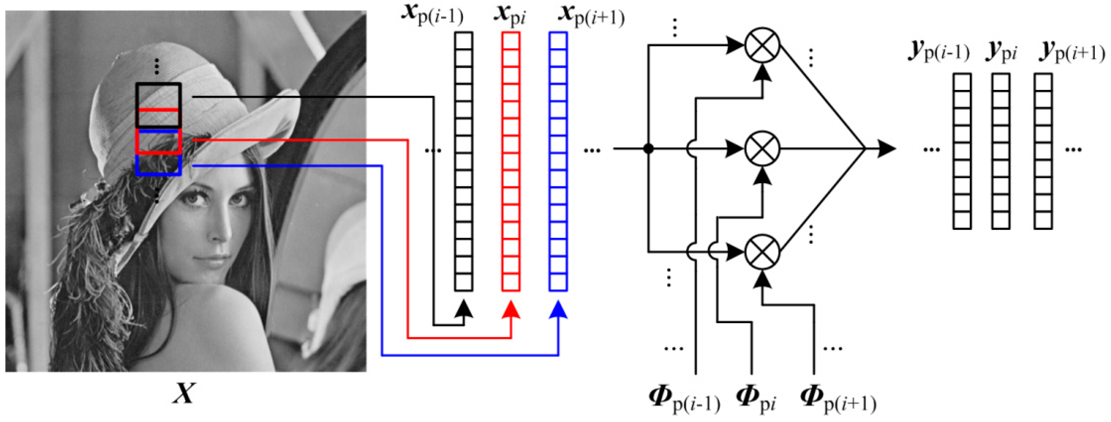
3.2. Patch Structure
BL performs the recovery algorithm block by block, any two blocks are different in recovery quality because the statistical characteristic of block is non-stationary. Blocking artifacts are usually perceived in the regions where one block has significantly different statistics from its neighbors. By extending BL, we present a patch structure (PA) which split the 2-D image into overlapping patches. As shown in Figure 4, PA first splits the 2-D image X into K overlapping blocks Xpi ∈ RP×P (Np = P × P), and transfer these patches to 1-D vector xpi ∈ through raster scanning. The size of overlap region between two neighboring patches is P/2, i.e., we slide a P×P patch in an image with the step size being P/2. By constructing the block measurement matrix Φpi ∈ , the CS measurements ypi ∈ of xpi are generated as
in which Mp is the number of CS measurements for each patch, and the subrate S can be computed by Mp/Np. The storage of Φpi is moderate, so PA cannot introduce for sensors excessive burdens of computing and storing. By the predictive quantizing, these measurements are transferred to bits, and transmitted to decoder. By replacing Φbi and ybi in Equation (6) with Φpi and ypi, the linear recovery algorithm is used to recover each patch, and these patches are spliced together into a whole image. PA smooths the boundary between two blocks, so it shows efficiency of reducing blocking artifacts.
3.3. Layered Structure
Blocking artifacts results from the differences of neighboring blocks in recovery quality. The smaller the block size is, the more serious blocking artifacts are. The recovery quality is known to be better with a large block [22], so blocking artifacts can be effectively suppressed when we set a large block size in BL. However, considering the light burden of sensor, a small block size is more desired. Especially for predictive quantization, a high spatial correlation exists among small-size blocks, which would increase predicting efficiency of quantization. In view of that, as shown in Figure 5, we present the layered structure (LA) which can splice CS measurements of small blocks into those of large blocks, thus enabling the measuring of small blocks and the recovery of large blocks.
In LA, we set a block-size pair (B1, B2), in which B1 and B2 are the block size for measuring and recovery, respectively. To achieve measuring small block and recovering large block, B1 is smaller than B2, and they satisfy that,
where l is a positive integer. When performing CS measuring, as the same with BL, LA splits the 2-D image X into L non-overlapping blocks Xbi ∈ (Nb = B1 × B1) and transfer these blocks to 1-D vector xbi ∈ through raster scanning. By constructing the block measurement matrix Φbi ∈ , the CS measurements ybi ∈ of these small blocks are produced, and we gather these CS measurements into the structure at the low layer. By re-organizing the low-layer structure, these CS measurements of small blocks are converted into those of large blocks which form the structure at high layer. The following describes the process of converting structure from low layer to high layer when l is set to be 1. As shown in Figure 5, each red block contains four black blocks which are measured as
and splice ybi into y in rows, i.e.,
in which Φ is the diagonal matrix composed of the block measurement matrices of four black blocks. These CS measurements of red blocks are gathered into the high-layer structure. However, from Equation (17), it can be seen that the column vector y does not correspond to the column vector x of the red block, so ΦΛ needs to be transformed into a proper matrix. By an elementary column transformation, it is easy to transform [xb1; xb2; xb3; xb4] into x, which can be represented as
in which E is an elementary column transformation matrix. Plugging Equation (18) into Equation (17), we can get
in which Θ = ΦΛE. According to Equation (19), we construct CS measuring formula of the red block, so we can use the CS measurements of black blocks to linearly recover the red ones by Equation (6). When l is set to be larger than 1, the construction of LA can be done in the manner similar to the above.
4. Experimental Results
In this section, we subjectively and objectively evaluate the reconstruction quality of some 512 × 512 test images using different measurement structures in image CS. These test images include Lenna, Barbara, Peppers, Goldhill, and Mandrill. In all experiments, the subrate S is set to be in the range of [0.1, 0.5]. For WH, DCT-based SRM [19] is used to construct the measurement matrix, SQ is used to quantize CS measurements, and GPSR algorithm is used to recover images. For BL, RA, PA, and LA, to ensure a fair comparison, i.i.d. Gaussian matrix is selected to be measurement matrix, DPCM is used to quantize CS measurements, and images are recovered linearly. The block size is set to be 16 in BL, and LA uses different block-size pairs in different experiments. Subjective evaluation shows the reconstructed images at different subrates using different structures. In objective evaluation, we measure the recovery quality in terms of peak signal-to-noise ratio (PSNR), bitrate, and encoding time. The variation of PSNR with bitrate is called rate-distortion, and the variation of PSNR with encoding time is called time-distortion. Bitrate indicates the size of data transmitted by sensor, and encoding time gives an indication of the amount of energy expended while encoding, so rate-distortion reflects the transmission efficiency, and time-distortion the energy efficiency. All experiments are conducted under the following computer configuration: Intel(R) Core (TM) [email protected] GHz CPU, 8 GB RAM, Microsoft Windows 764 bits, and MATLAB Version 7.6.0.324 (R2008a).
4.1. Subjective Evaluation
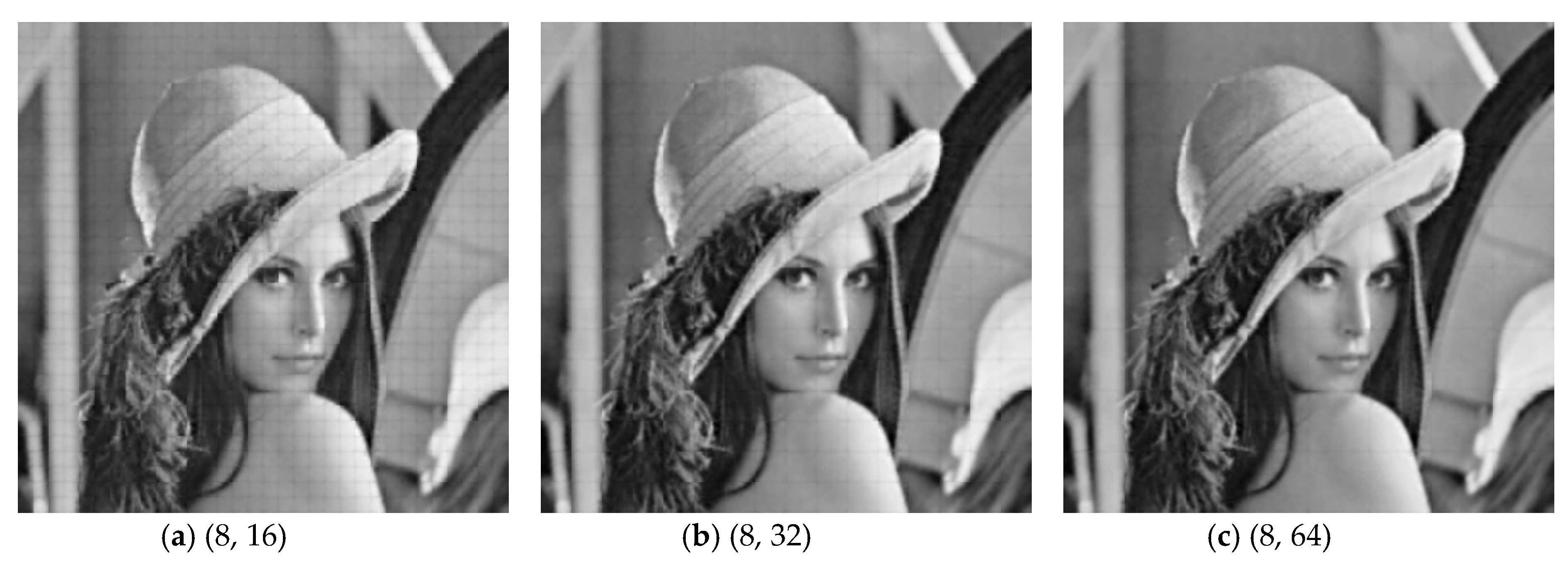
Figure 6 presents the visual recovery results of Lenna by various measurement structures at different subrates. When subrate S is 0.1, due to insufficient CS measurements, the reconstructed image by any structure lose structural details. It can be seen that, WH presented a disappointing result due to serious blurs, and BL bring lots of blocking artifacts. Although RA and PA can remove the blocking artifacts, they introduce other problems—e.g., obvious stripes in RA, global fuzzy in PA. When setting the block-size pair (8, 16), LA has a good visual perception when compared with BL, though many blocking artifacts still exist. When subrate S is increased to be 0.3, bad effects can be efficiently suppressed in WH, PA, and RA, and blocking artifacts almost disappear in BL and LA. When subrate S is 0.5, all structures provide satisfying visual results. we can see from the above that, none of the structures can guarantee good visual results when subrate S is 0.1, therefore, we expect to improve the visual quality at a low subrate. As shown in Figure 7, with a large l, LA can satisfy our expectation. When l is set to be 2, i.e., the block-size pair is (8, 32), blocking artifacts are reduced efficiently at subrate S = 0.1, and even when the block-size pair is (8, 64), blocking artifacts are almost imperceptible. When setting a small block size, as shown in Figure 7d–f, LA can still ensure a high efficiency for reducing blocking artifacts. Given the above, LA has greater potential than other structures from subjective view.
4.2. Objective Evaluation
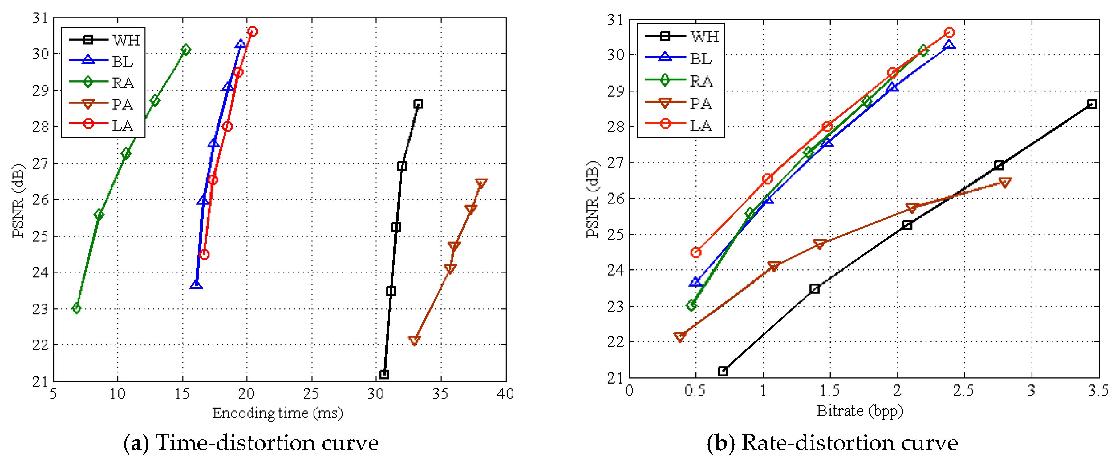
Table 2 presents the average encoding time of various structures on all test images when setting different subrates. WH and PA have a high execution time at any subrate, and their average time is respectively 31.74 and 36.05 ms on all subrates. BL, RA, and LA have a low execution time, among which RA does the best with only 10.86 ms on all subrates. Table 3 presents the average decoding time of various structures on all test images at different subrates. We can see that, the decoding time of WH is much longer than those of other structures, indicating that the non-linear recovery brings a heavy burden for WH. Due to linear recovery, BL, RA, PA, and LA all have a low decoding time, especially for LA, with only 6.03 ms at all subrates. Table 2 and Table 3 both considered, we can see that LA is a good structure for green IoT because it guarantees a low complexity at both encoder and decoder. Figure 8 shows average time-distortion and rate-distortion curves on test images for various measurement structures. It can be seen that, WH and PA have a poor time-distortion performance due to high encoding time, the time-distortion performance of BL is close to that of LA, and RA works the best among all structures. As for rate-distortion performance, WH and PA perform poorly, and LA works the best among all structures. Although RA has a good time-distortion performance, it produces more bits than LA. Figure 9 shows average time-distortion and rate-distortion curves on test images for LA structures with various block-size pairs. It can be seen that the rate-distortion performance can be significantly improved when block size B1 of measuring is much smaller than block size B2 of recovery, but different block-size pairs have little impact on time-distortion performance. To sum up, LA can save more bits while keeping both a low encoding time and a good recovery quality. Given the positive relation between encoding time and energy consumption, LA is the most suitable one among all structures for Green IoT from the objective view.
4.3. Effects of Measurement Matrices
In this section, we present the effects of different measurement matrices on the performance of BL, RA, PA, and LA. We select two classic measurement matrices, Gaussian matrix and permuted fast Fourier transform (PFFT) matrix [30], and two hardware-friendly matrices, ±Bernoulli matrix [31] and DCT-based SRM [19]. To ensure a fair comparison, all structures use linear algorithm to reconstruct test images. Table 4 presents the average encoding time of various structures on all test images at all subrates using different measurement matrices. It can be seen that, no matter which matrix is used, RA costs less encoding time than other structures, PA requires the most time among all structures, and BL and LA have a moderate encoding complexity. For any structure, the encoding time varies slightly even when different matrices are used. Table 5 presents the average PSNR values of various structures on all test images at all subrates using different measurement matrices. It can be seen that LA gets higher PSNR values than others regardless of matrix used. For any structure, Gaussian matrix provides higher PSNR values than others, and ±Bernoulli and SRM matrices have a little PSNR degradation compared with Gaussian matrix. We can find from the above that both encoding time and imaging quality considered, LA provides a good balance for any measurement matrix, and ±Bernoulli and SRM matrices have little effect on the performance of different structures compared with Gaussian matrix. In order to make LA hardware-friendly, therefore, Gaussian matrix can be replaced with ±Bernoulli and SRM matrices.
4.4. Effects of Recovery Algorithms
In this section, we present the effects of different recovery algorithms on the performance of different structures. All structures use DCT-based SRM to measure test images. The four recovery algorithms, namely GPSR, orthogonal matching pursuit (OMP) [32], Bayesian recovery [33], and linear recovery, are used to reconstruct test images. To ensure good performance of non-linear algorithms, the block size is set to be 32 for BL and PA, and the block-size pair of LA is set to be (32, 64). Table 6 presents the average decoding time of different structures on all test images at all subrates using different recovery algorithms. We can see that non-linear algorithms cost far more decoding time than linear algorithm for any structure, and LA costs more decoding time than BL, RA, PA, for linear algorithm, indicating that linear algorithm has a light computational burden compared with non-linear algorithms, and LA increases the decoding computation. Table 7 presents the average PSNR values of different structures on all test images at all subrates using different recovery algorithms. It can be seen that linear algorithm provides higher PSNR values than non-linear algorithms for any structure, especially that LA cooperated with linear recovery achieves the highest PSNR value. From the above, we can find that linear algorithm is more suitable for BL, RA, PA, and LA in terms of either computational complexity or objective quality, and LA can improve the recovery quality at the cost of some computational burden increase.
5. Conclusions
In this paper, we have reviewed two traditional measurement structures of image CS, i.e., WH and BL, and propose three potential structures for Green IoT, i.e., RA, PA, and LA. As a straightforward structure, WH stores CS measurements of a whole image at a time, but must use SRM to measure and recover image in order to avoid the huge storage and computations. BL organizes CS measurements block by block, with high energy efficiency and low storage, but it produces serious blocking artifacts at the low subrate. By replacing non-overlapping block in BL with raster and overlapping block, RA and PA can remove blocking artifacts, though bringing other problems. LA splits image into small blocks, and re-organizes these measurements of small blocks into those of large ones. Since small block improves the efficiency of predictive quantization, and large block enhances the recovery quality, LA can efficiently suppress blocking artifacts. We perform several experiments to evaluate the subjective and objective performances of all structures. At a low subrate, by setting a proper block-size pair, LA almost eliminates blocking artifacts, and provides better visual quality than other structures. It shows good time-distortion and rate-distortion performances, especially for rate-distortion performance, it can significantly improve it by setting a large block size of recovering. Both subjective and objective evaluation considered, it can be seen that LA is the most suitable for green IoT among structures.
This paper only presents an exploratory research, and there are many intriguing questions that future work should consider. For instance, for PA, a patch overlaps its neighbors, so we can design more efficient recovery algorithm by using the correlation among patches. Also, parallel computing can be adopted to speed up the linear recovery for LA.
Author Contributions
R.L. contributed to the concept of the research, performed the data analysis and wrote the manuscript; X.D. helped perform the data analysis with constructive discussions and helped performed the experiment. Y.L. revised the manuscript, and provided the necessary support for the research.
Funding
This work was supported in part by the National Natural Science Foundation of China, under grant nos. 61501393 and 61572417, in part by Nanhu Scholars Program for Young Scholars of Xinyang Normal University, and in part by Innovation Team Support Plan of University Science and Technology of Henan Province (no. 19IRTSTHN014).
Conflicts of Interest
The authors declare no conflict of interest.
References
- Baraniuk, R.G.; Goldstein, T.; Sankaranarayanan, A.C.; Studer, C.; Veeraraghavan, A.; Wakin, M.B. Compressive video sensing: Algorithms, architectures, and applications. IEEE Signal Process. Mag. 2017, 34, 52–66. [Google Scholar] [CrossRef]
- Candè, E.J.; Wakin, M.B. An introduction to compressive sampling. IEEE Signal Process. Mag. 2008, 25, 21–30. [Google Scholar] [CrossRef]
- Mun, S.; Fowler, J.E. Motion-compensated compressed-sensing reconstruction for dynamic MRI. In Proceedings of the 2013 IEEE International Conference on Image Processing, Melbourne, Australia, 15–18 September 2013; pp. 1006–1010. [Google Scholar]
- Li, C.; Sun, T.; Kelly, K.F.; Zhang, Y. A compressive sensing and unmixing scheme for hyperspectral data processing. IEEE Trans. Image Process. 2012, 21, 1200–1210. [Google Scholar] [PubMed]
- Wu, J.; Liu, F.; Jiao, L.C.; Wang, X. Compressive sensing SAR image reconstruction based on Bayesian framework and evolutionary computation. IEEE Trans. Image Process. 2011, 20, 1904–1911. [Google Scholar] [CrossRef] [PubMed]
- Bevacqua, M.T.; Crocco, L.; Donato, L.D.; Isernia, T. Non-linear inverse scattering via sparsity regularized contrast source inversion. IEEE Trans. Comput. Imaging 2017, 3, 296–304. [Google Scholar] [CrossRef]
- Bevacqua, M.T.; Isernia, T. Boundary indicator for aspect limited sensing of hidden dielectric objects. IEEE Geosci. Remote Sens. Lett. 2018, 15, 838–842. [Google Scholar] [CrossRef]
- Morabito, A.F. Synthesis of maximum-efficiency beam arrays via convex programming and compressive sensing. IEEE Antennas Wirel. Propag. Lett. 2017, 16, 2404–2407. [Google Scholar] [CrossRef]
- Morabito, A.F.; Rocca, P. Reducing the number of elements in phase-only reconfigurable arrays generating sum and difference patterns. IEEE Antennas Wirel. Propag. Lett. 2015, 14, 1338–1341. [Google Scholar] [CrossRef]
- Arshad, R.; Zahoor, S.; Shah, M.A.; Wahid, A.; Yu, H. Green IoT: An investigation on energy saving practices for 2020 and beyond. IEEE Access 2017, 5, 15667–15681. [Google Scholar] [CrossRef]
- Hu, J.; Luo, J.; Zheng, Y.; Li, K. Graphene-grid deployment in energy harvesting cooperative wireless sensor networks for Green IoT. IEEE Trans. Ind. Inform. 2018. [Google Scholar] [CrossRef]
- Colonnese, S.; Biagi, M.; Cattai, T.; Cusani, R.; De Vico Fallani, F.; Scarano, G. Green compressive sampling reconstruction in IoT networks. Sensors 2018, 18, 2735. [Google Scholar] [CrossRef] [PubMed]
- Chen, P.; Ahammad, P.; Boyer, C.; Huang, S.I.; Lin, L.; Lobaton, E.; Meingast, M.; Oh, S.; Wang, S.; Yan, P.; et al. CITRIC: A low-bandwidth wireless camera network platform. In Proceedings of the ACM/IEEE International Conference on Distributed Smart Cameras, Stanford, CA, USA, 7–11 September 2008; pp. 1–10. [Google Scholar]
- Asif, M.S.; Fernandes, F.; Romberg, J. Low-complexity video compression and compressive sensing. In Proceedings of the 2013 Asilomar Conference on Signals, Systems and Computers, Pacific Grove, CA, USA, 3–6 November 2013; pp. 579–583. [Google Scholar]
- Figueiredo, M.A.T.; Nowak, R.D.; Wright, S.J. Gradient projection for sparse reconstruction: Application to compressed sensing and other inverse problems. IEEE J. Sel. Top. Signal Process. 2007, 1, 586–597. [Google Scholar] [CrossRef]
- Bioucas-Dias, J.M.; Figueiredo, M.A.T. A new TwIST: Two-step iterative shrinkage/thresholding algorithms for image restoration. IEEE Trans. Image Process. 2007, 16, 2992–3004. [Google Scholar] [CrossRef]
- Becker, S.; Bobin, J.; Candès, E.J. NESTA: A fast and accurate first-order method for sparse recovery. SIAM J. Imaging Sci. 2011, 4, 1–39. [Google Scholar] [CrossRef]
- Beck, A.; Teboulle, M. A fast iterative shrinkage-thresholding algorithm for linear inverse problems. SIAM J. Imaging Sci. 2009, 2, 183–202. [Google Scholar] [CrossRef]
- Do, T.T.; Gan, L.; Nguyen, N.H.; Tran, T.D. Fast and efficient compressive sensing using structurally random matrices. IEEE Trans. Signal Process. 2012, 60, 139–154. [Google Scholar] [CrossRef]
- Zhang, P.; Gan, L.; Sun, S.; Ling, C. Modulated unit-norm tight frames for compressed sensing. IEEE Trans. Signal Process. 2015, 63, 3974–3985. [Google Scholar] [CrossRef]
- Hsieh, S.H.; Lu, C.S.; Pei, S.C. Compressive sensing matrix design for fast encoding and decoding via sparse FFT. IEEE Signal Process. Lett. 2018, 25, 591–595. [Google Scholar] [CrossRef]
- Gan, L. Block compressed sensing of natural images. In Proceedings of the 2007 15th International Conference on Digital Signal Processing, Cardiff, UK, 1–4 July 2007; pp. 403–406. [Google Scholar]
- Mun, S.; Fowler, J.E. Block compressed sensing of images using directional transforms. In Proceedings of the 2009 16th IEEE International Conference on Image Processing, Cairo, Egypt, 7–10 November 2009; pp. 3021–3024. [Google Scholar]
- Yu, Y.; Wang, B.; Zhang, L. Saliency-based compressive sampling for image signals. IEEE Signal Process. Lett. 2010, 17, 973–976. [Google Scholar]
- Zhang, J.; Xiang, Q.; Yin, Y.; Chen, C.; Luo, X. Adaptive compressed sensing for wireless image sensor networks. Multimedia Tools and Applications. Multimed. Tools Appl. 2017, 76, 4227–4242. [Google Scholar] [CrossRef]
- Mun, S.; Fowler, J.E. DPCM for quantized block-based compressed sensing of images. In Proceedings of the 2012 Proceedings of the 20th European Signal Processing Conference, Bucharest, Romania, 27–31 August 2012; pp. 1424–1428. [Google Scholar]
- Wang, L.; Wu, X.; Shi, G. Binned progressive quantization for compressive sensing. IEEE Trans. Image Process. 2012, 21, 2980–2990. [Google Scholar] [CrossRef] [PubMed]
- Dinh, K.Q.; Shim, H.J.; Jeon, B. Measurement coding for compressive imaging using a structural measuremnet matrix. In Proceedings of the 2013 IEEE International Conference on Image Processing, Melbourne, Australia, 15–18 September 2013; pp. 10–13. [Google Scholar]
- Gao, X.; Zhang, J.; Che, W.; Fan, X.; Zhao, D. Block-based compressive sensing coding of natural images by local structural measurement matrix. In Proceedings of the 2015 Data Compression Conference, Snowbird, UT, USA, 7–9 April 2015; pp. 133–142. [Google Scholar]
- Duarte, M.; Wakin, M.; Baraniuk, R. Fast reconstruction of piecewise smooth signals from incoherent projections. Presented at the Workshop on Signal Processing with Adaptive Sparse Structured Representations, Rennes, France, 16–18 November 2005; pp. 1–4. [Google Scholar]
- Baraniuk, R.; Davenport, M.; DeVore, R. A simple proof of the restricted isometry property for random matrices. Constr. Approx. 2008, 28, 253–263. [Google Scholar] [CrossRef]
- Tropp, J.A.; Gilbert, A.C. Signal recovery from random measurements via orthogonal matching pursuit. IEEE Trans. Inf. Theory 2007, 53, 4655–4666. [Google Scholar] [CrossRef]
- Ji, S.; Xue, Y.; Carin, L. Bayesian compressive sensing. IEEE Trans. Signal Process. 2008, 56, 2346–2356. [Google Scholar] [CrossRef]
Figure 1.
Illustration on WH format.

Figure 2.
Illustration on BL format.

Figure 3.
Illustration on RA format.

Figure 4.
Illustration on PA format.

Figure 5.
Illustration on LA format. The block-size pair is (B1, B2), and B2/B1 is 2.

Figure 6.
Visual quality comparison on test image Lenna for various measurement structures. Note: the block-size pair of LA is (8, 16).
Figure 6.
Visual quality comparison on test image Lenna for various measurement structures. Note: the block-size pair of LA is (8, 16).


Figure 7.
Visual quality comparison on test image Lenna for LA structures with various block-size pairs when the subrate is 0.1.
Figure 7.
Visual quality comparison on test image Lenna for LA structures with various block-size pairs when the subrate is 0.1.


Figure 8.
Average time-distortion and rate-distortion curves on test images for various measurement structures. Note: the block-size pair of LA is (8, 16).
Figure 8.
Average time-distortion and rate-distortion curves on test images for various measurement structures. Note: the block-size pair of LA is (8, 16).

Figure 9.
Average time-distortion and rate-distortion curves on test images for LA structures with various block-size pairs.
Figure 9.
Average time-distortion and rate-distortion curves on test images for LA structures with various block-size pairs.


Table 1.
List of acronyms and notations.
| CS | Compressive Sensing |
| Green IoT | Green Internet of Things |
| WH | Whole Structure |
| BL | Block Structure |
| RA | Raster Structure |
| PA | Patch Structure |
| LA | Layered Structure |
| SQ | Scalar Quantization |
| DPCM | Differential Pulse Code Modulation |
| SRM | Structurally Random Matrix |
| DCT | Discrete Cosine Transform |
| FFT | Fast Fourier Transform |
| GPSR | Gradient Projection for Sparse Reconstruction |
| PSNR | Peak Signal-to-Noise Ratio |
Table 2.
Execution time (ms) of encoder for various measurement structures.
| Subrate | 0.1 | 0.2 | 0.3 | 0.4 | 0.5 | Average |
|---|---|---|---|---|---|---|
| WH | 30.68 | 31.17 | 31.57 | 31.97 | 33.28 | 31.74 |
| BL | 16.09 | 16.63 | 17.46 | 18.57 | 19.52 | 17.65 |
| RA | 6.82 | 8.57 | 10.69 | 12.91 | 15.31 | 10.86 |
| PA | 33.01 | 35.72 | 36.06 | 37.36 | 38.12 | 36.05 |
| LA | 16.66 | 17.37 | 18.46 | 19.31 | 20.41 | 18.44 |
Note: the block-size pair of LA is (8, 16).
Table 3.
Execution time (ms) of decoder for various measurement structures.
| Subrate | 0.1 | 0.2 | 0.3 | 0.4 | 0.5 | Average |
|---|---|---|---|---|---|---|
| WH | 1.22 × 10⁵ | 1.00 × 10⁵ | 0.65 × 10⁵ | 0.52 × 10⁵ | 0.31 × 10⁵ | 0.74 × 10⁵ |
| BL | 10.12 | 10.21 | 10.16 | 10.14 | 10.33 | 10.19 |
| RA | 5.67 | 7.92 | 8.66 | 10.05 | 12.88 | 9.04 |
| PA | 21.18 | 21.71 | 21.92 | 21.72 | 21.59 | 21.62 |
| LA | 5.39 | 5.69 | 6.03 | 6.51 | 6.54 | 6.03 |
Note: the block-size pair of LA is (8, 16).
Table 4.
Average execution time (ms) of encoder for different structures using different measurement matrices.
Table 4.
Average execution time (ms) of encoder for different structures using different measurement matrices.
| Gaussian | PFFT | ±Bernoulli | SRM | |
|---|---|---|---|---|
| BL | 17.65 | 18.35 | 18.14 | 18.17 |
| RA | 10.86 | 11.13 | 10.67 | 10.66 |
| PA | 36.05 | 34.23 | 33.11 | 33.28 |
| LA | 18.44 | 18.71 | 18.14 | 18.61 |
Note: the block-size pair of LA is (8, 16).
Table 5.
Average PSNR values (dB) for different structures using different measurement matrices.
| Gaussian | PFFT | ±Bernoulli | SRM | |
|---|---|---|---|---|
| BL | 27.28 | 25.70 | 26.88 | 26.69 |
| RA | 26.94 | 16.22 | 26.92 | 26.94 |
| PA | 24.63 | 24.22 | 24.38 | 24.24 |
| LA | 27.82 | 26.09 | 27.53 | 27.48 |
Note: the block-size pair of LA is (8, 16).
Table 6.
Average execution time (ms) of decoder for different measurement structures using different recovery algorithms.
Table 6.
Average execution time (ms) of decoder for different measurement structures using different recovery algorithms.
| GPSR | OMP | Bayesian | Linear | |
|---|---|---|---|---|
| WH | 7.44 × 10⁴ | -- | -- | -- |
| BL | 9.34 × 10⁴ | 5.57 × 10³ | 6.26 × 10⁴ | 114.36 |
| RA | 9.00 × 10⁴ | 5.56 × 10³ | 6.64 × 10⁴ | 127.11 |
| PA | 1.14 × 10⁵ | 2.99 × 10³ | 7.73 × 10⁴ | 71.97 |
| LA | 5.32 × 10⁵ | 1.70 × 10⁵ | 2.14 × 10⁵ | 3.94 × 10³ |
Note: due to the unavailability of function handle, OMP, Bayesian and linear algorithms cannot be used for WH.
Table 7.
Average PSNR values (dB) for different measurement structures using different recovery algorithms.
Table 7.
Average PSNR values (dB) for different measurement structures using different recovery algorithms.
| GPSR | OMP | Bayesian | Linear | |
|---|---|---|---|---|
| WH | 25.08 | -- | -- | -- |
| BL | 22.93 | 23.07 | 24.13 | 28.01 |
| RA | 19.80 | 20.63 | 21.63 | 26.94 |
| PA | 21.03 | 21.61 | 21.57 | 25.44 |
| LA | 23.04 | 23.32 | 24.47 | 28.12 |
Note: due to the unavailability of function handle, OMP, Bayesian and linear algorithms cannot be used for WH.
© 2018 by the authors. Licensee MDPI, Basel, Switzerland. This article is an open access article distributed under the terms and conditions of the Creative Commons Attribution (CC BY) license (http://creativecommons.org/licenses/by/4.0/).
Share and Cite
MDPI and ACS Style
Li, R.; Duan, X.; Li, Y. Measurement Structures of Image Compressive Sensing for Green Internet of Things (IoT). Sensors 2019, 19, 102. https://doi.org/10.3390/s19010102
AMA Style
Li R, Duan X, Li Y. Measurement Structures of Image Compressive Sensing for Green Internet of Things (IoT). Sensors. 2019; 19(1):102. https://doi.org/10.3390/s19010102
Chicago/Turabian StyleLi, Ran, Xiaomeng Duan, and Yanling Li. 2019. "Measurement Structures of Image Compressive Sensing for Green Internet of Things (IoT)" Sensors 19, no. 1: 102. https://doi.org/10.3390/s19010102
Note that from the first issue of 2016, this journal uses article numbers instead of page numbers. See further details here.