1. Introduction
The placement of sensors significantly affects the performance of identification, state estimation as well as fault detection and isolation (FDI) algorithms. The goal-oriented placement of sensors for dynamical systems is a challenging task [
1]. Parameter estimation-oriented information entropy-based optimal sensor placement was investigated in [
2]. Based on robust information entropy, a Bayesian sequential sensor placement algorithm for multi-type of sensor is also proposed [
3]. Computational Fluid Dynamics (CFD) models were generated to predict wind-flow that used the data of a sensor placement utilised with prediction-value joint entropy [
4]. For fault detection and isolation, an incremental analytical redundancy relation (ARR)-based algorithm was introduced in [
5]. Structural analysis-based sensor placement strategies place additional sensors to isolate otherwise undisguisable faults [
6]. In the initial sensor-constrained problems, the number of sensors is given and the detection time has to be minimized [
7], while, as far as time-constrained problems are concerned, the aim is to minimize the number of required sensors that ensure a predefined detection time. In the case of dynamical systems, the previously mentioned detection time is related to the relative degree of the system [
8]. Besides good FDI performance, the optimal placement of the sensors should also ensure the observability of the systems [
9].
Network representation-based structural controllability and observability analysis of dynamical systems is a hot topic in literature [
10,
11,
12,
13,
14,
15,
16] since the introduction of this new approach [
17]. The methodology utilizes the maximum matching algorithm to determine the minimum set of actuators and sensors required to grant structural controllability and observability for an arbitrary dynamical system. Although the results are very promising, the methodology can overestimate the number of necessary actuators [
18] when the details of the edge dynamic are neglected [
14].
When the observability analysis of the system is performed on a properly defined network, the problem concerning the observability analysis is reduced to a reachability problem [
19]. In some cascaded systems, this highlights that the number of necessary sensors is significantly smaller than the size of the state variables, which makes the observation vulnerable and the relative degree, i.e., the minimum number of derivatives that is necessary to observe at least one signal of inputs, is very high. To deal with the vulnerability, Liu et al. proposed a methodology to grant robustness in the undirected representation of the system [
20].
There is an almost infinite number of objectives that can be used to define a sensor placement problem [
21]. In most of the cases, the optimization problem is formulated as that the instrumentation cost should be minimized and the precision of reconciled values should be ensured in a reliable, resilient and robust manner [
22]. As the problem is NP-hard (non-deterministic polynomial-time hard), the mixed-integer programming-based approach is suitable to small-to-medium sized networks [
23]. To handle the complexity of the problem, a heuristic approach is mostly followed. For example, to reconstruct the internal states of biochemical reaction systems with the minimum number of sensors, a graphical method has been developed [
24]. Among population-based optimization algorithms, genetic algorithms (GAs) are the most frequently applied, e.g., GA was utilized to find a sensor configuration that minimizes cost and maximizes the reliability and observability of the system [
25]. The main benefit of these gradient-free heuristic optimization methods is that they can be utilized with a wide range of models [
26]. Simulated annealing (SA) is also widely employed optimization algorithm in sensor placement [
27]. SA lends itself to be combined with other search algorithms, e.g., with local search heuristics [
28] or other SA inner loop, which results in dual representation simulated annealing (DRSA) [
29]. These techniques are often combined also in sensor placement, e.g., GA and SA were successfully integrated [
30]. Recently, Particle Swarm Optimization (PSO) was applied in an optimal sensor location problem (OSLP) [
31] and in the design of an ultrasonic Structural Health Monitoring (SHM) system [
32]. According to these publications, heuristic optimization techniques are efficient in finding a small number of sensors with less time-consuming computations [
33].
In this paper, to ensure observability and minimize the relative order of dynamical systems, two methodologies for sensor placement are introduced. The presented methods combine the metaheuristic SA optimization method with clustering. SA is chosen as it exhibits excellent levels of performance with regard to graph-represented combinatorial optimization (CO). The use of simulated annealing is strengthened by the fact that the relative degree of the system can be interpreted as a path in a network, and simulated annealing models a random walk on the search graph. Based on this concept, SA was applied to place micro-hydropowers in a water supply network [
34] and network alignment in biological systems [
35].
As sensors practically group the observed state variables, sensor placement can be considered as a special
k-medoid clustering problem. This concept has been utilized in Ref. [
36], where fuzzy c-means clustering algorithm was utilized to characterize the spatial distribution of the sensor placement problem.
The Clustering Large Applications (CLASA) algorithm [
37] developed as a fast and robust solution to the well-known
k-medoid clustering problem. The fundamental idea of the paper is that instead of considering the distance between the cluster centers and the clustered objects, a goal-oriented sensor-placement algorithm can be derived by the introduction of a problem-relevant objective function into the scheme of the CLASA algorithm. The second novelty of the paper is that the random search of the resulted algorithm is fine-tuned by calculating the selection probabilities based on network distance-related fuzzy membership functions.
The structure of the paper is the following. In
Section 2.1, the theoretical foundations and nomenclature of the relative degree of multiple-input and multiple-output (MIMO) dynamical systems are introduced.
Section 2.2 presents the maximum matching-based sensor placement algorithm that ensures structural observability. In
Section 2.3, the proposed optimization algorithms are introduced.
Section 3 provides examples of application. Finally,
Section 4 concludes the paper.
2. Sensor Placement to Ensure Observability and Minimal Relative Order
In
Section 2.1, the relative degree of MIMO systems is defined and the sensor placement task is considered to be an optimization problem.
Section 2.2 presents the first step of our methodology, which places the sensors as the structural observability of the system is guaranteed.
Section 2.3 presents the proposed simulated annealing-based clustering algorithms that optimally place the additional sensors to minimize the relative degree of the system.
2.1. Problem Formulation
A nonlinear MIMO system can be represented by state-space model:
where the vectors
,
and
stand for the state variables, inputs and outputs, respectively.
The model can be linearized and the resultant linear approximation represented by a linear state-space model [
38]:
When the number of state variables is denoted by
N, the number of actuators by
M and the number of sensors by
K, then the matrices
,
and
define how state variables influence each other, how the actuators influence the state variables, and how the sensors record the state variables, respectively.
For each pair of output and input ( and ), the relative degree of the system can be defined as the minimum number of derivatives of that is directly influenced by the change in . The relative degree for an arbitrary output i is defined as , which requires the observer to observe the effect of at least one of the inputs.
When the aim of the observer is to estimate the effect of the
disturbance vector that independently influences all state variables,
then
is an identity matrix
and the relative order of the system is
.
As
Figure 1 illustrates the relative degree of an
state variable can be interpreted as the
length of the path between the
j-th state variable and the nearest sensor,
, selected as
, while the relative order of the whole system is defined by the maximum of these minimal distances.
As the generation of a balanced placement of sensors is of interest, the set of sensor nodes
S is determined by minimizing the following cost function:
where parameter
weights between the maximum and the balance-related average of the relative order of the system.
2.2. Placing Sensors to Ensure Observability
Besides the minimisation of the relative order, the observability of the system should also be ensured. Based on the Kalman rank criterion, a linear dynamical system is said to be structurally observable, if and only if the observability matrix
is of full rank (
) [
39].
Based on the state-transition matrix
, a graph
can be constructed where the set of vertices
V represent the state variables and the edges
are determined by the nonzero elements of
(see
Figure 2). In the graph representation, the relative degree
can be defined as the distance between the input/disturbance
and the output
, which is the distance between the
j-th and
i-th nodes in the directed network
, so the the optimization problem can be considered as a special graph partitioning problem. This graph-based representation is beneficial as the maximum matching of
can be used to determine the minimal number and places of the sensor nodes that are required to ensure the observability of the system.
As directed graphs can be represented as bipartite graphs, the maximum matching of the related bipartite graph was studied [
14,
17]. The endpoints of the directed edges in
are the matched nodes (
), while others are the unmatched nodes (
), thus
. Based on [
17], the unmatched nodes
of
, where
E is determined by
, define the driver nodes, i.e., where the actuators should be placed. Furthermore, unmatched nodes of
, where
E is defined by
, should be the sensor nodes. In other words, the nodes where sensors should be placed. If the determined driver nodes or sensor nodes are assigned to the system, then it becomes a structurally controllable or structurally observable system [
14]. As the aim of this paper is to deal with system observability,
was used with the adjacency matrix based on
. To ensure the structural observability of the system, the path-finding method was used to define the minimum number of mandatory sensors and their location [
14].
In order to generate the output matrix such that the relative order is minimal and the system observable, first the unmatched set of nodes is generated, followed by the set of candidate sensor nodes . The cardinality of the candidate sensor nodes is (). The resulting is designed based on the set of sensor nodes such that for each , is a one-hot row vector whose i-th element is non-zero, so .
As the number of sensors which can be allocated without any restrictions is , different combinations of possible placements of sensors exists. To solve this NP-hard problem, simulated annealing-based heuristic optimization algorithms are proposed in the following section.
2.3. Simulated Annealing and Fuzzy Clustering-based Output Configuration Design
To optimize the relative order and smoothness of these orders, the objective function (Equation (
7)), which can be considered as a linear combination of the maximum and average distance of the sensors from the observed state variables was defined. Based on this interpretation, the minimisation problem can also be seen as a
k-medoid clustering problem, where the centroid elements are the sensor nodes and the members of the clusters are the observed state variables.
To determine the locations of the additional sensors two approaches are proposed inspired by Clustering Large Applications based on Simulated Annealing algorithm (CLASA) [
37] and the Geodesic Distance-based Fuzzy
c-Medoid Clustering method (GDFCM) [
40]. In the first algorithm, the CLASA algorithm is modified as follows. The original objective function of CLASA that calculates the distances between the objects and the medoids (in our case, the distances between the state variables and the sensors) is replaced by what was proposed in Equation (
7). With the new objective function, not just the minimum relative order can be granted, but different sensor configurations with the same relative order can be distinguished to balance the load of the sensors. The search mechanism should be fine-tuned as the medoids of the fixed sensors (
) have fixed positions to ensure the observability of the system. The second algorithm enhances the random search of the resulted mCLASA algorithm by the introduction of distance-dependent selection probability calculated based on the Geodesic Distance-based Fuzzy
c-Medoid Clustering method (GDFCM) [
40].
In both algorithms, firstly the fixed sensor nodes are determined to grant the observability property based on the unmatched set of nodes. Then, the candidate sensor nodes are generated randomly, and the cost is calculated. Following this, in each iteration, one of the candidate sensor nodes () is randomly changed, and the new cost is calculated. From this, the difference between the new cost and the previously applied cost is calculated (). The new placement of the sensors is accepted if .
If
, the worsened placement of the sensor is accepted only with the probability defined as
, where
denotes the temperature of the cooling process of the SA in iteration
i, whose dynamics can be seen in Equation (
8). This randomization of the search allows for the algorithm to explore the search space and converge with the increase of the number of iterations:
The pseudo code of the proposed modified Clustering Large Applications based on Simulated Annealing algorithm (mCLASA) can be seen in Algorithm 1. The algorithm possesses the following inputs and parameters:
G denotes the network representation of the system from Equation (
5),
stands for the parameter of the cost function from Equation (
7),
represents the number of additional sensors,
is the number of iterations of the simulated annealing,
denotes the maximum, i.e., the initial temperature, and
stands for the minimum temperature. The following values were used for the parameters:
,
,
and
.
| Algorithm 1 Pseudo code of the modified CLASA algorithm (mCLASA). |
- 1:
proceduremCLASA(G, , , , , ) - 2:
, - 3:
▷ using the path finding method: [ 14] - 4:
Let be the set of the randomly chosen elements from - 5:
▷Equation ( 7) - 6:
for to do - 7:
Let be a randomly selected element from - 8:
- 9:
Let be a randomly chosen node from - 10:
- 11:
- 12:
- 13:
if then - 14:
- 15:
- 16:
else - 17:
if then - 18:
- 19:
- 20:
end if - 21:
end if - 22:
- 23:
end for - 24:
return - 25:
end procedure
|
The second method utilizes the GDFCM method [
40] to extend the previously introduced mCLASA method. This extension increases the probability that in each iteration potentially better neighboring sensors are selected to replace the sensors placed in the previous iteration steps
. The algorithm considers the sensors as cluster centers (medoids), determines the cluster assignments of the state variables, and swaps the medoid (the sensor) with a randomly selected state variable. The random selection utilizes distance-based fuzzy membership values. The cluster memberships
of the state variables
are determined by the fuzzy membership function (see Equation (
9) in the description of the algorithm), where the distances are calculated in the undirected version of the graph (
). A roulette wheel selection [
41] selects the new medoid according to the membership values. The search space of the algorithm is also controlled by the fuzzy exponent
m which is decreased in each iteration by
, in the same manner as
in Equation (
8).
The pseudo code of the suggested Geodesic Distance-based Fuzzy c-medoid Clustering with Simulated Annealing algorithm (GDFCMSA) can be seen in Algorithm 2. The algorithm possesses the following inputs and parameters: G denotes the network representation of the system, stands for the balance parameter of the cost function, represents the number of additional sensors, is the number of iterations of the simulated annealing, denotes the maximum fuzzy component value and stands for the minimum fuzzy component value. The following values were used for the parameters: , , , , and .
| Algorithm 2 Pseudo code of the Geodesic Distance-based Fuzzy c-Medoid Clustering with Simulated Annealing algorithm (GDFCMSA). |
- 1:
procedureGDFCMSA(G, , , , , , , ) - 2:
, , , - 3:
▷ using the path finding method: [ 14] - 4:
Let be the set of the randomly chosen state elements from - 5:
▷ Equation ( 7) - 6:
for to do - 7:
Calculate the fuzzy membership values for , and :
- 8:
Let be a randomly selected sensor node from - 9:
- 10:
- 11:
for all do - 12:
- 13:
end for - 14:
- 15:
- 16:
- 17:
- 18:
if then - 19:
- 20:
- 21:
else - 22:
if then - 23:
- 24:
- 25:
end if - 26:
end if - 27:
, - 28:
end for - 29:
return - 30:
end procedure
|
4. Conclusions
To ensure the structural observability in addition to fast and robust observer response, two clustering- and simulated annealing-based methods were proposed.
Additional sensors are placed into the system based on the CLASA algorithm by the mCLASA algorithm. The placements of additional sensors is further improved by the Geodesic Distance-based Fuzzy c-Medoid Clustering with Simulated Annealing algorithm (GDFCMSA) as their positioning is based on a geodesic distance-based fuzzy membership functions. Simulated annealing is applied by both algorithms to minimize the cost function, which in turn minimizes the maximum and average of the relative orders of the system to generate a balanced placement of sensors.
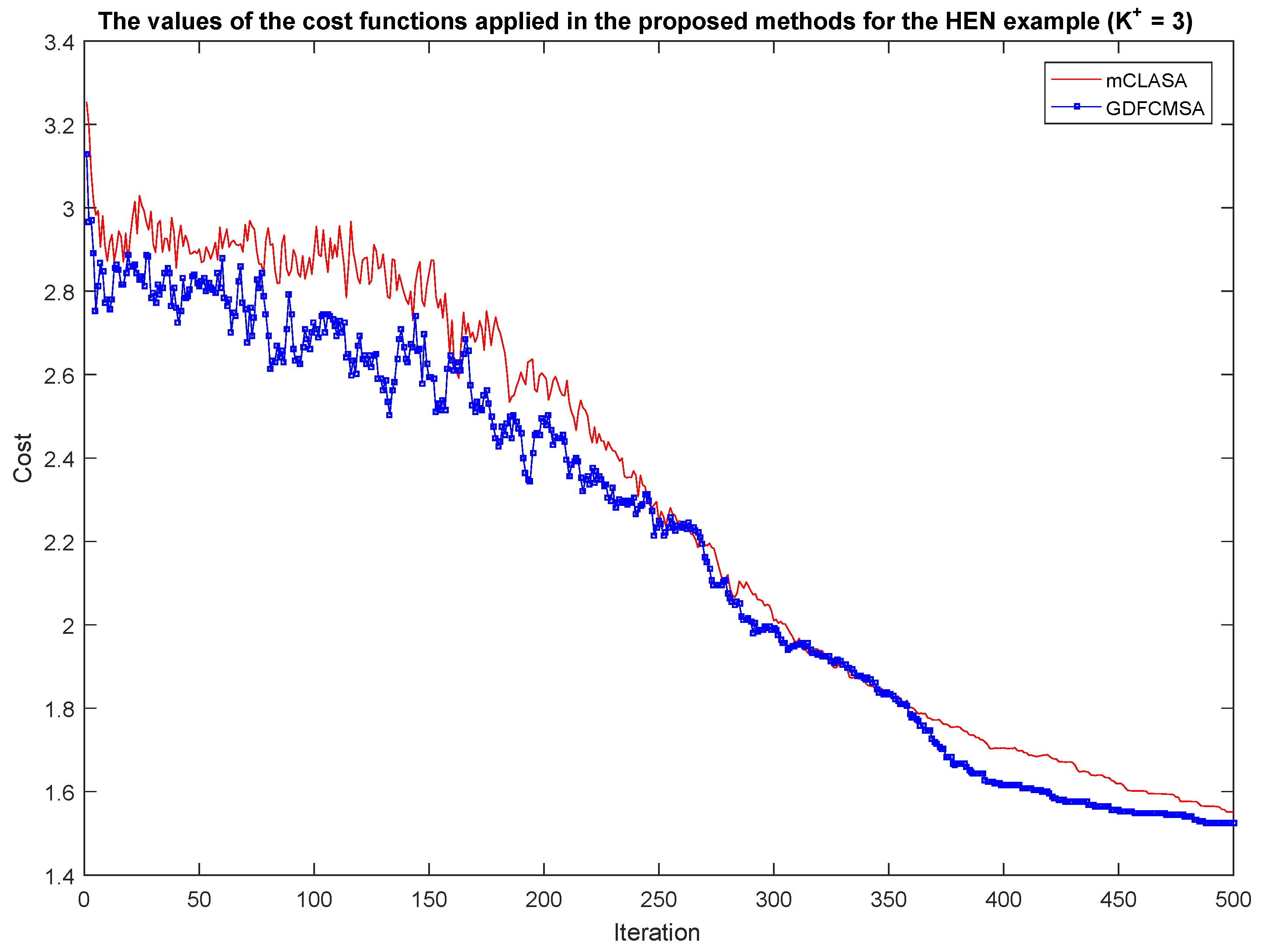
A slightly better solution is provided by the GDFCMSA algorithm than the mCLASA method at the expense of some additional computational resources for the evaluation of the membership degrees. Solutions to massive problems are generated by both methods over a short period of time, which illustrates the applicability of these methods in an industrial setting.
Although this paper deals with the placement of sensors, the proposed methodology can be applied to control configuration design as well, since this is the dual problem of the design of the output configuration.


