Vehicle Collision Prediction under Reduced Visibility Conditions


Abstract
1. Introduction
2. Related Work
2.1. Research on Collision Warning Models
2.2. Research on Human Factors
- Perception is “the time to see or discern an object or event”.
- Intellection is “the time to understand the implications of the object’s presence or event”.
- Emotion is “the time to decide how to react”.
- Volition is “the time to initiate the action, for example, the time to engage the brakes”.
2.3. Research on Vehicle Speed Prediction
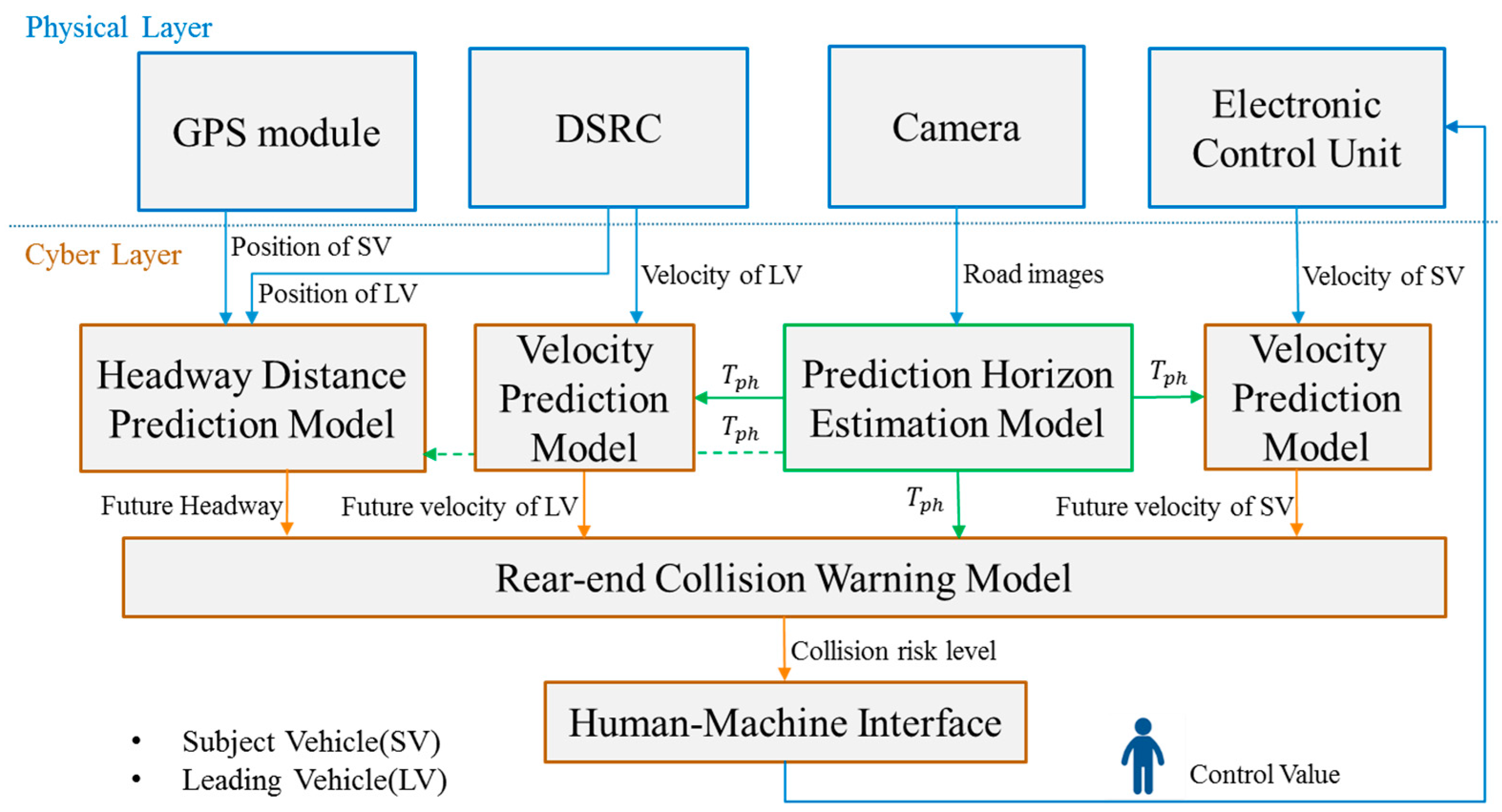
3. Visibility-Based Collision Warning System Design
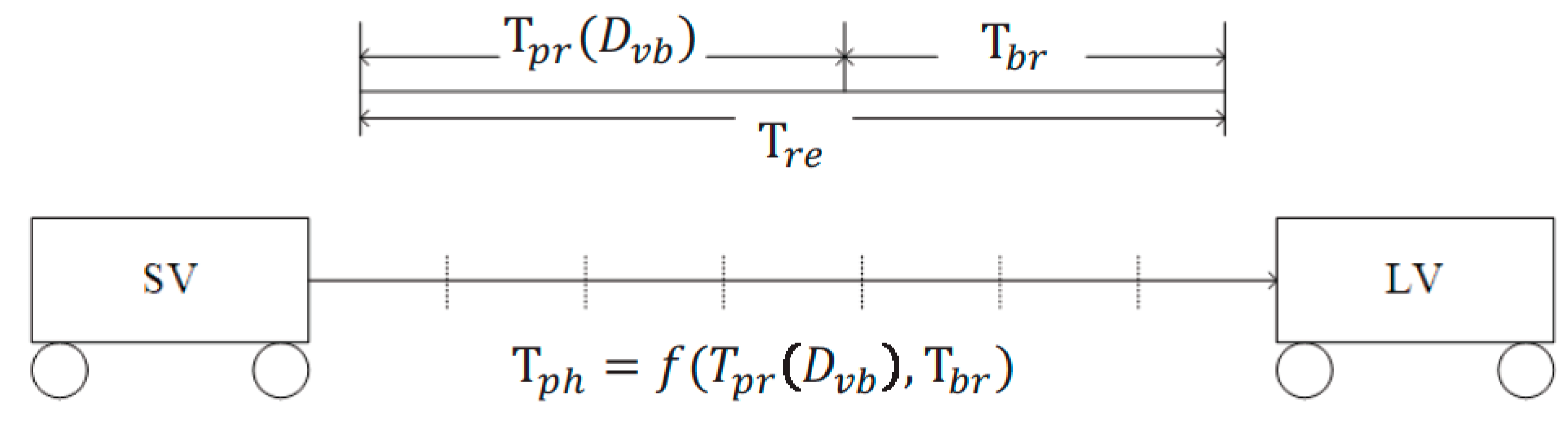
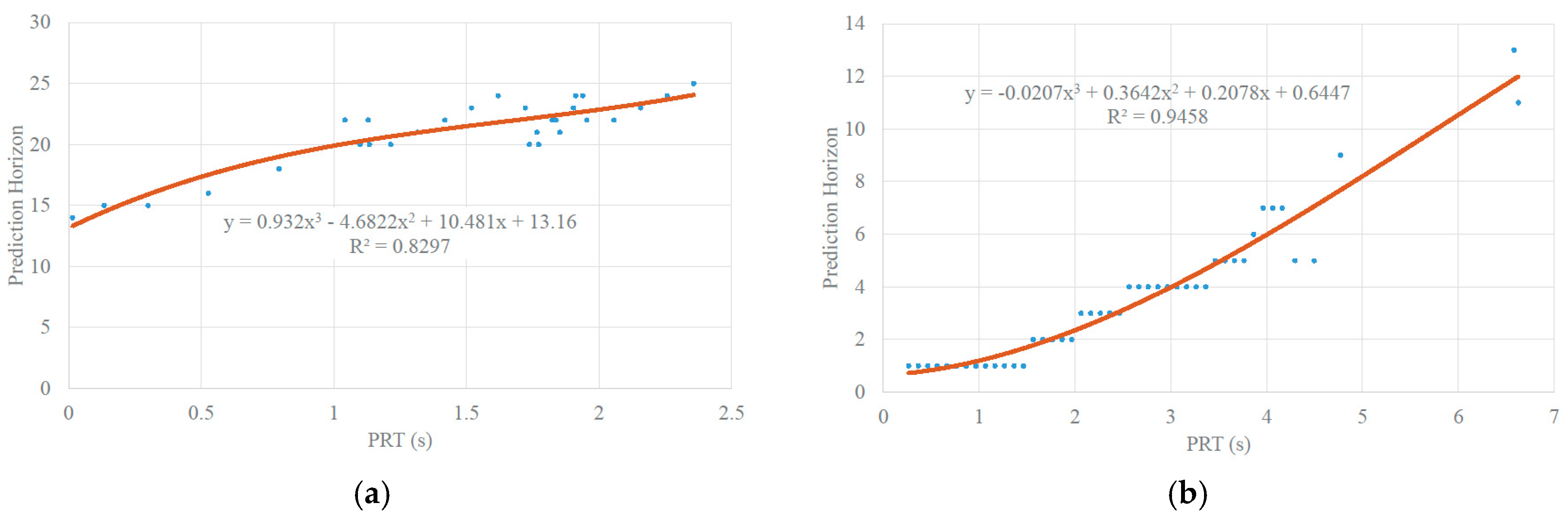
3.1. Prediction Horizon Estimation Model
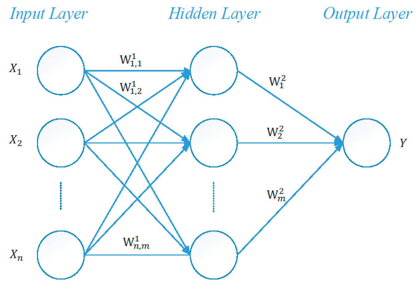
3.2. Velocity Prediction Model
3.3. Headway Distance Prediction Model
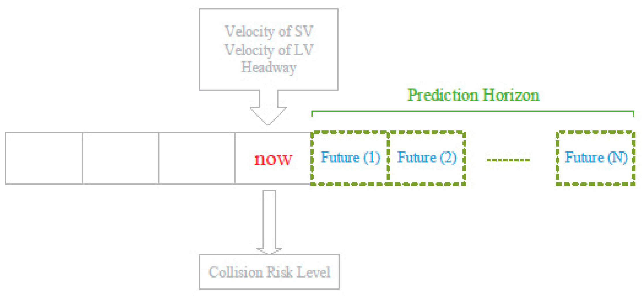
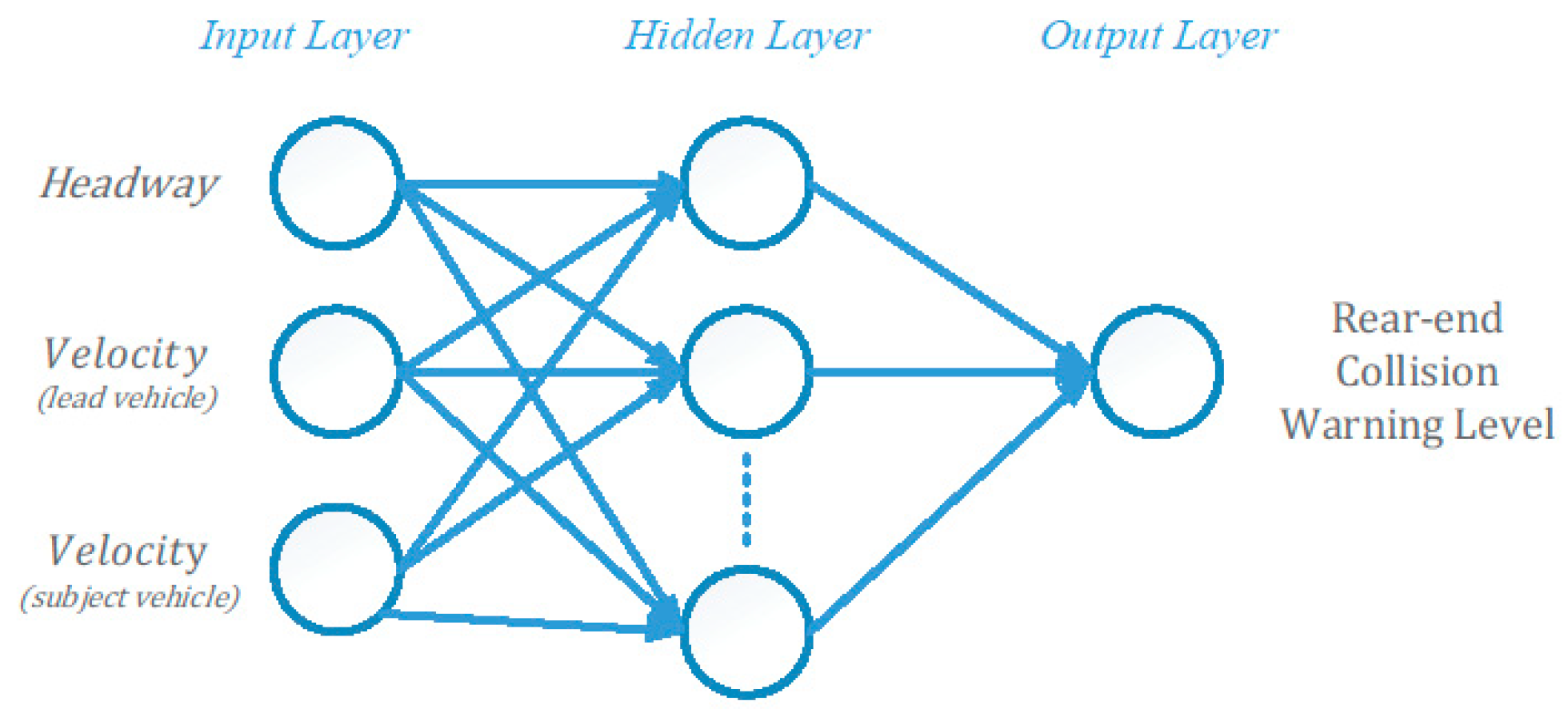
3.4. Rear-End Collision Warning Model
4. Experiments
4.1. Test Data
4.2. Experiment Results
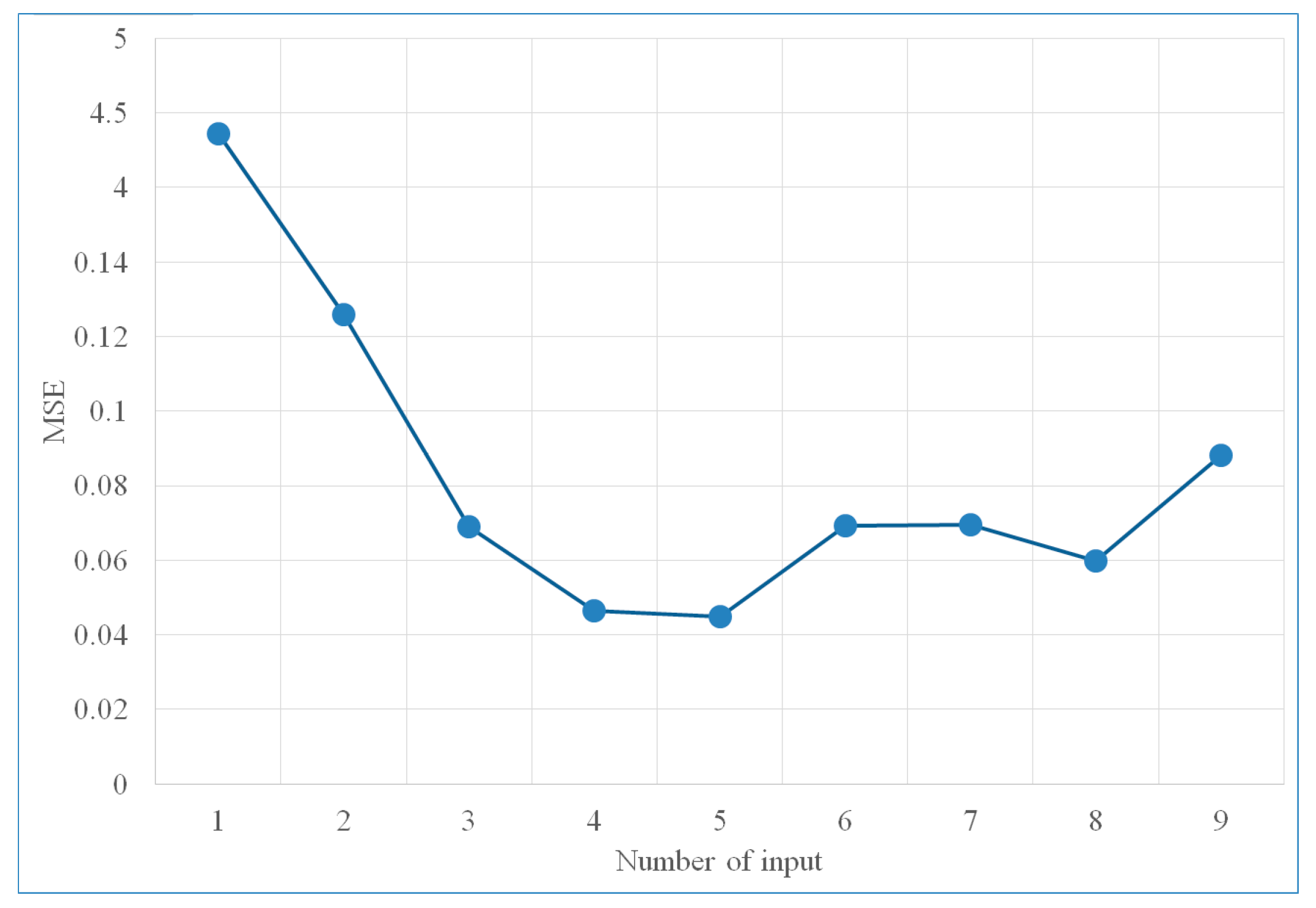
4.2.1. Deciding the Number of Training Inputs for Velocity Prediction Model
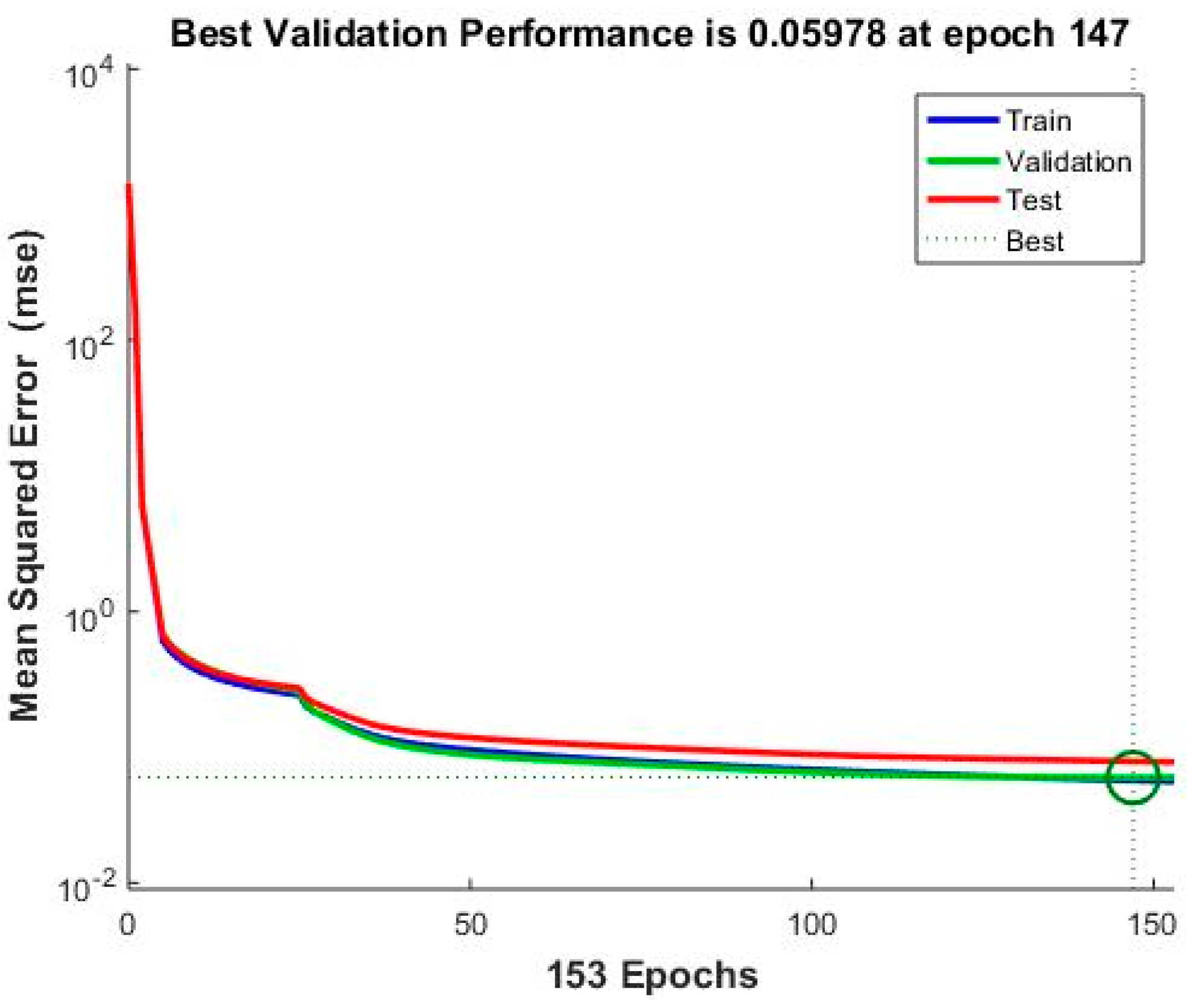
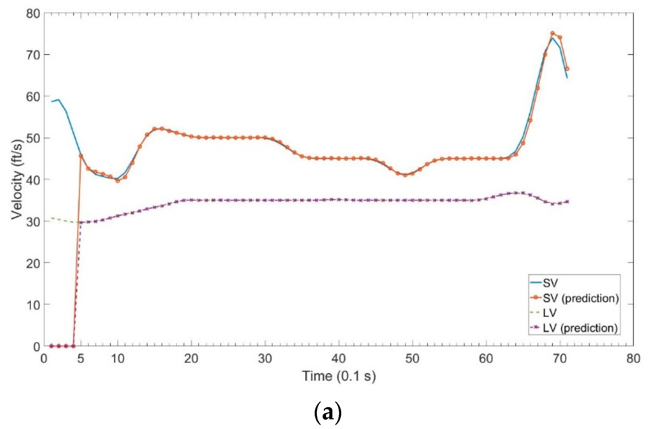
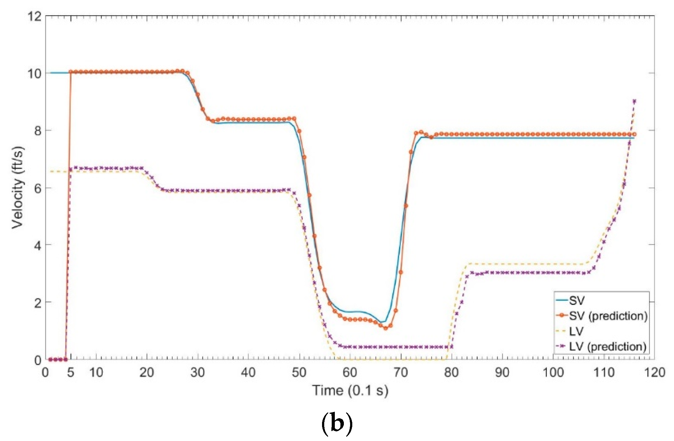
4.2.2. Velocity Prediction Results
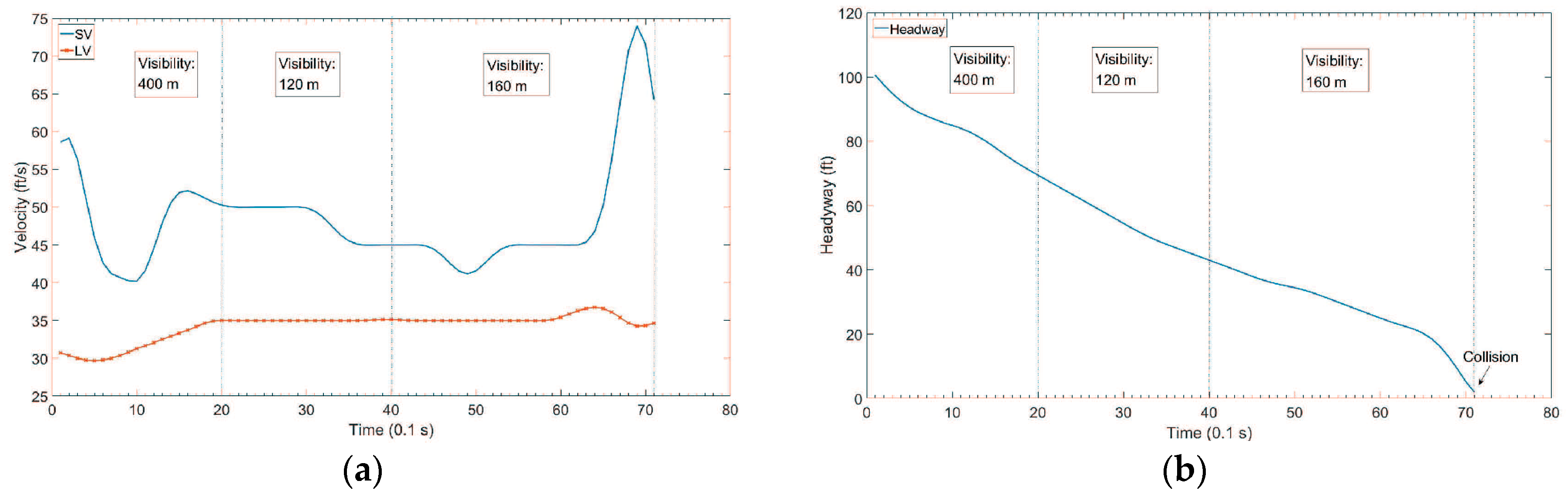
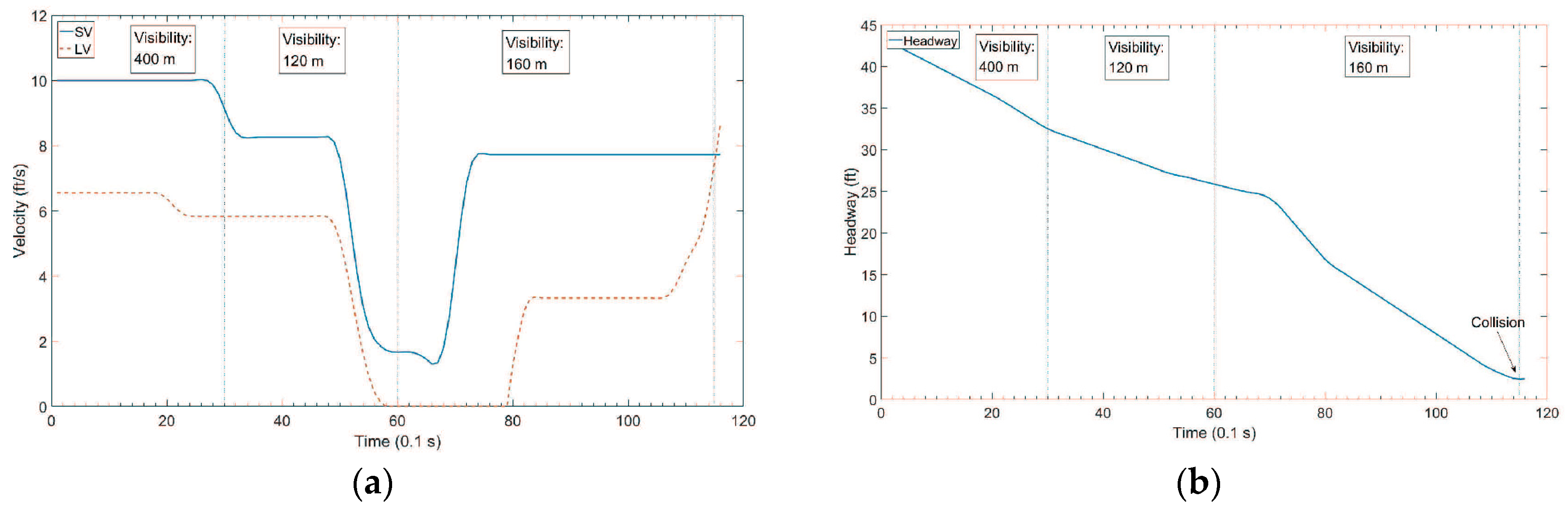
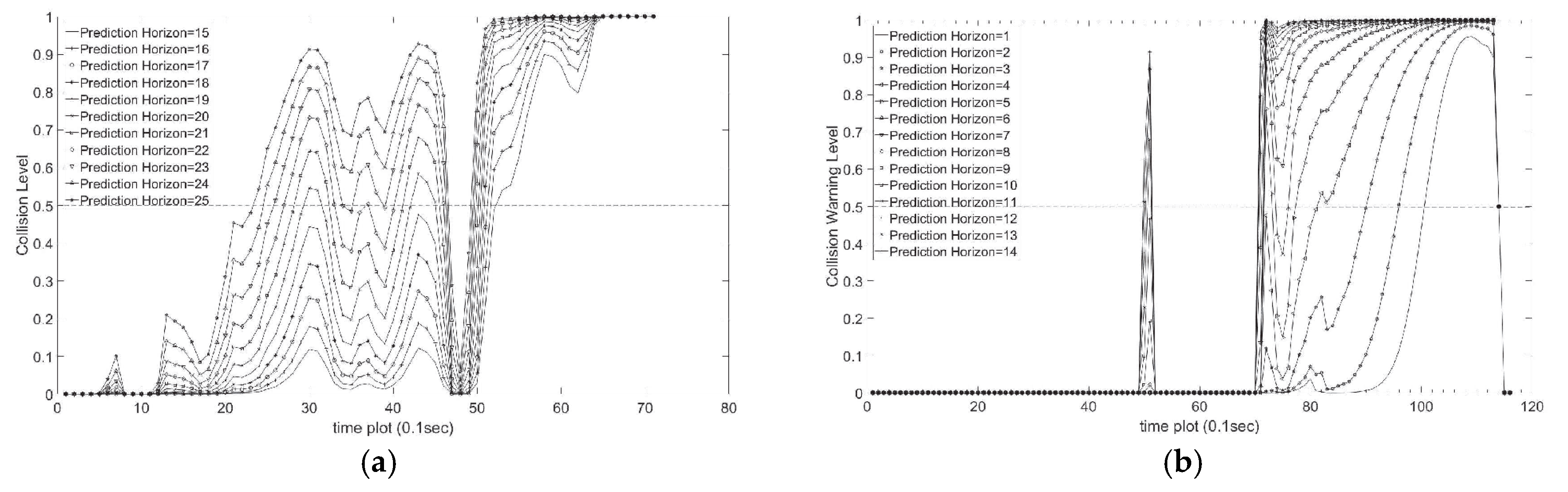
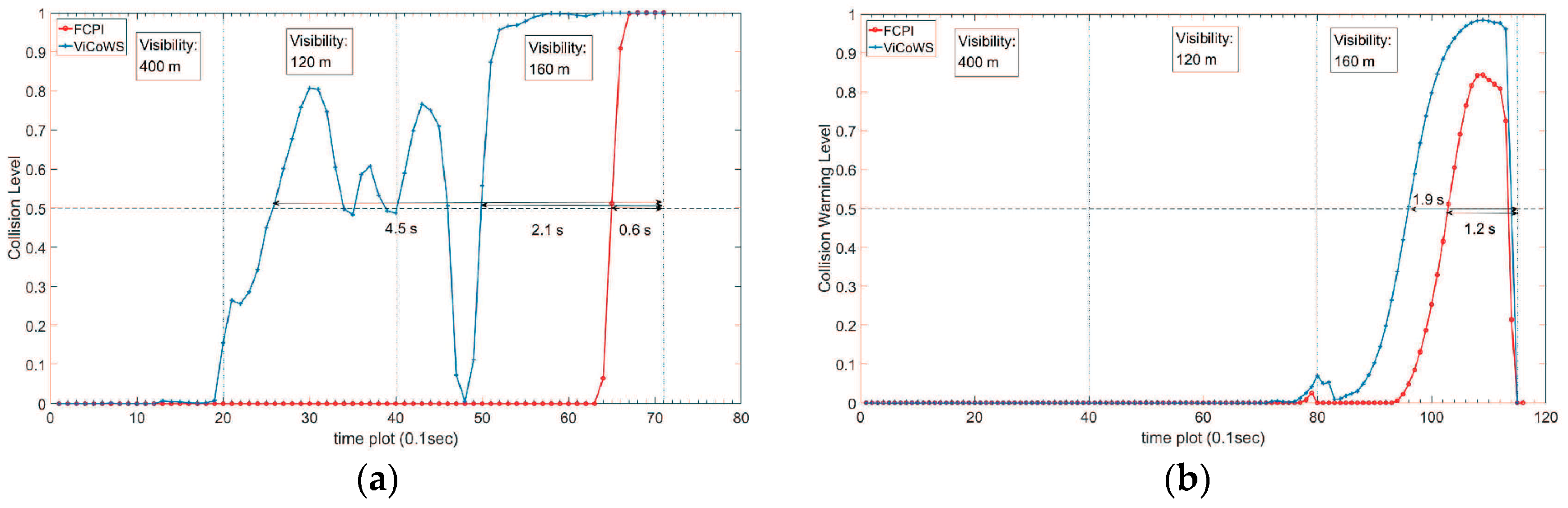
4.2.3. Collision Warning with Different Prediction Horizons
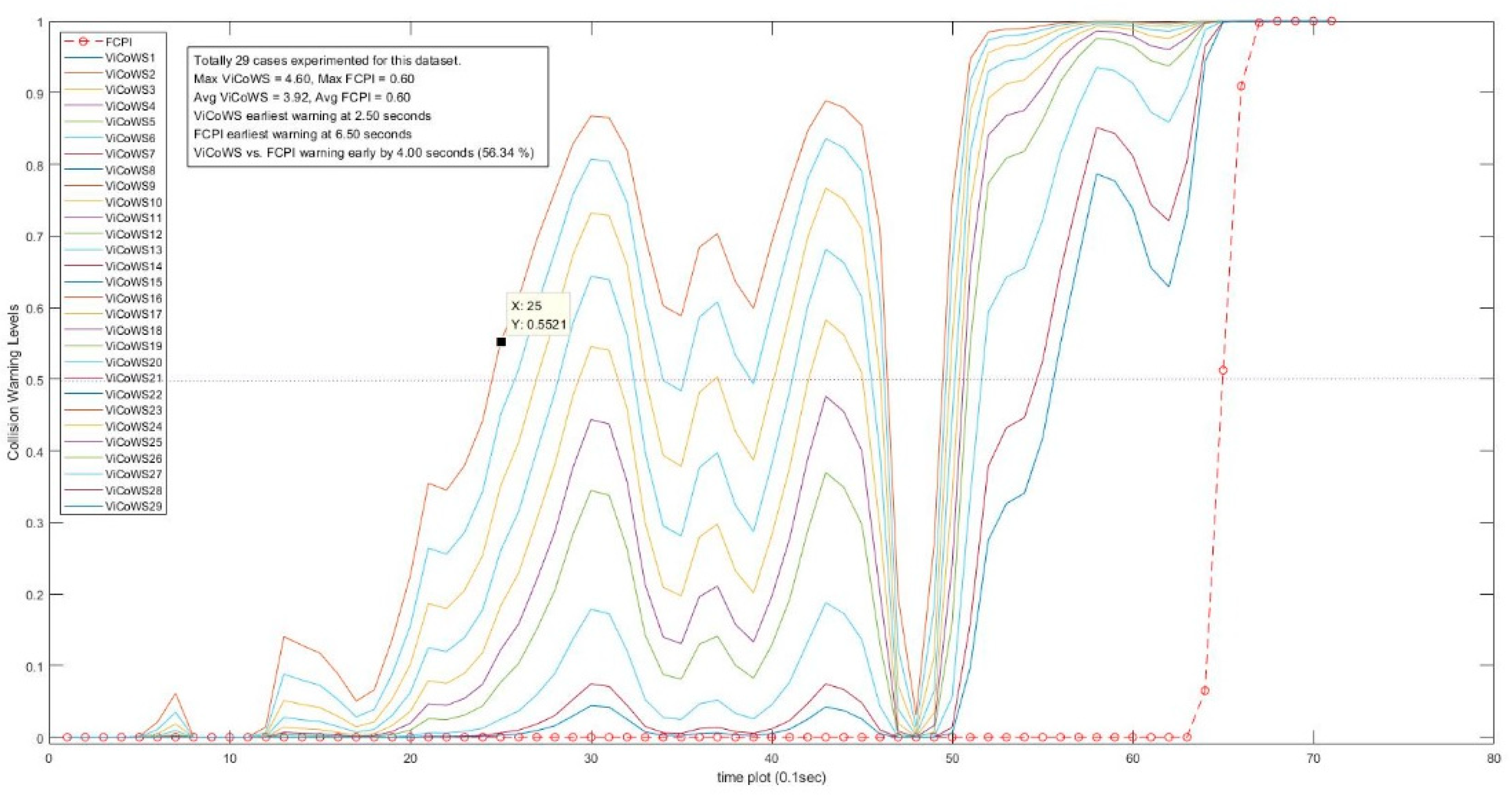
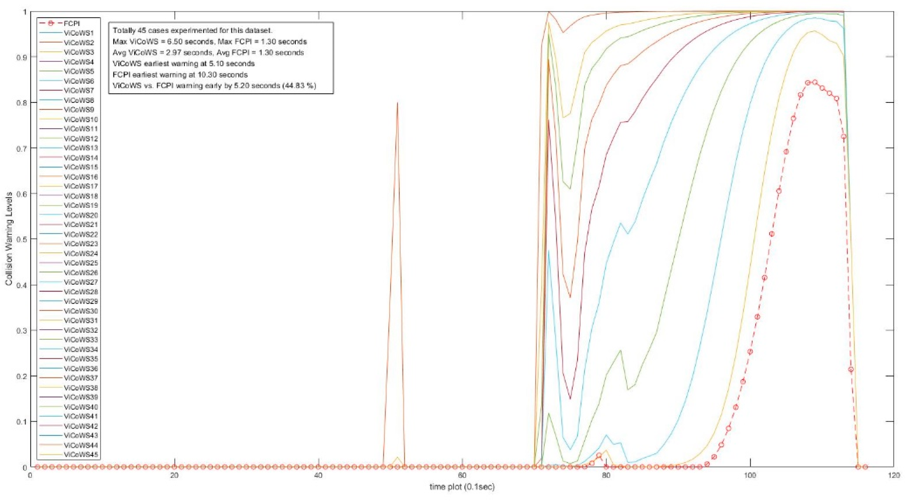
4.2.4. Comparison with Different Methods
5. Conclusions
Author Contributions
Funding
Conflicts of Interest
References
- 2014 Traffic Safety Facts FARS/GES Annual Report; DOT HS 812 261; National Highway Traffic Safety Administration, U.S. Department of Transportation: Washington, DC, USA, 2016. Available online: http://www-nrd.nhtsa.dot.gov/Pubs/812261.pdf (accessed on 24 July 2018).
- Yamada, Y.; Tokoro, S.; Fujita, Y. Development of a 60 GHz radar for rear-end collision avoidance. In Proceedings of the Intelligent Vehicles Symposium, Paris, France, 24–26 October 1994; pp. 207–212. [Google Scholar]
- Rasshofer, R.H.; Spies, M.; Spies, H. Influences of weather phenomena on automotive laser radar systems. Adv. Radio Sci. 2011, 9, 49–60. [Google Scholar] [CrossRef]
- Jiang, D.; Delgrossi, L. IEEE 802.11p: Towards an international standard for wireless access in vehicular environments. In Proceedings of the Vehicular Technology Conference, Singapore, 11–14 May 2008; pp. 2036–2040. [Google Scholar]
- Dalla Chiara, B.; Deflorio, F.; Diwan, S. Assessing the effects of inter-vehicle communication systems on road safety. IET Intell. Transp. Syst. 2009, 3, 225–235. [Google Scholar] [CrossRef]
- Lee, D.; Yeo, H. Real-time rear-end collision-warning system using a multilayer perceptron neural network. IEEE Trans. Intell. Transp. Syst. 2016, 17, 3087–3097. [Google Scholar] [CrossRef]
- Wu, Z.; Liu, Y.; Pan, G. A smart car control model for brake comfort based on car following. IEEE Trans. Intell. Transp. Syst. 2009, 10, 42–46. [Google Scholar]
- Hayward, J.C. Near miss determination through use of a scale of danger. In Proceedings of the 51st Annual Meeting of the Highway Research Board, Washington, DC, USA, 17–21 January 1972; p. 2434. [Google Scholar]
- An, N.; Mittag, J.; Hartenstein, H. Designing fail-safe and traffic efficient 802.11p-based rear-end collision avoidance. In Proceedings of the IEEE Vehicular Networking Conference, Paderborn, Germany, 3–5 December 2014; pp. 9–16. [Google Scholar]
- Xiang, X.; Qin, W.; Xiang, B. Research on a DSRC-based rear-end collision warning model. IEEE Trans. Intell. Transp. Syst. 2014, 15, 1054–1065. [Google Scholar] [CrossRef]
- Grigoryev, V.; Khvorov, I.; Raspaev, Y.; Grigoreva, E. Intelligent transportation systems: Techno-economic comparison of dedicated UHF, DSRC, Wi-Fi and LTE access networks: Case study of St. Petersburg, Russia. In Proceedings of the Conference of Telecommunication, Media and Internet Techno-Economics, Munich, Germany, 9–10 November 2015; pp. 1–8. [Google Scholar]
- An, J.; Choi, B.; Hwang, T.; Kim, E. A novel rear-end collision warning system using neural network ensemble. In Proceedings of the IEEE Intelligent Vehicles Symposium, Gothenburg, Sweden, 19–22 June 2016; pp. 1265–1270. [Google Scholar]
- Wu, Y.; Abdel-Aty, M.; Lee, J. Crash risk analysis during fog conditions using real-time traffic data. Accid. Anal. Prev. 2018, 114, 4–11. [Google Scholar] [CrossRef] [PubMed]
- Wu, Y.; Abdel-Aty, M.; Cai, Q.; Lee, J.; Park, J. Developing an algorithm to assess the rear-end collision risk under fog conditions using real-time data. Transp. Res. Part C Emerg. Technol. 2018, 87, 11–25. [Google Scholar] [CrossRef]
- Layton, R.; Dixon, K. Stopping Sight Distance; Kiewit Center for Infrastructure and Transportation, Oregon Department of Transportation: Salem, OR, USA, 2012. [Google Scholar]
- Seiler, P.; Song, B.; Hedrick, J.K. Development of a collision avoidance system. In Proceedings of the Society of Automotive Engineers Conference, Detroit, MI, USA, 23–26 February 1998; pp. 97–103. [Google Scholar]
- Chang, B.R.; Tsai, H.F.; Young, C.P. Intelligent data fusion system for predicting vehicle collision warning using vision/GPS sensing. Expert Syst. Appl. 2010, 37, 2439–2450. [Google Scholar] [CrossRef]
- Kusano, K.D.; Gabler, H.C. Safety benefits of forward collision warning, brake assist, and autonomous braking systems in rear-end collisions. IEEE Trans. Intell. Transp. Syst. 2012, 13, 1546–1555. [Google Scholar] [CrossRef]
- Halmaoui, H.; Joulan, K.; Hautire, N.; Cord, A.; Brmond, R. Quantitative model of the driver’s reaction time during daytime fog—Application to a head up display-based advanced driver assistance system. IET Intell. Transp. Syst. 2015, 9, 375–381. [Google Scholar] [CrossRef]
- Graves, N.; Newsam, S. Using visibility cameras to estimate atmospheric light extinction. In Proceedings of the IEEE Workshop on Applications of Computer Vision, Kona, HI, USA, 5–7 January 2011; pp. 577–584. [Google Scholar]
- Negru, M.; Nedevschi, S. Image based fog detection and visibility estimation for driving assistance systems. In Proceedings of the IEEE International Conference on Intelligent Computer Communication and Processing, Cluj-Napoca, Romania, 5–7 September 2013; pp. 163–168. [Google Scholar]
- Zhang, S.; Tang, J. Study on the dynamic relationships between weather conditions and free-flow characteristics on freeways in Jilin. In Proceedings of the IEEE International Conference on Intelligent Transportation Systems, Hague, The Netherlands, 6–9 October 2013; pp. 1493–1498. [Google Scholar]
- Van Der Horst, R.; Hogema, J. Time-to-collision and collision avoidance systems. In Proceedings of the 6th International Co-operation on Theories and Concepts in Traffic Safety Workshop: Safety Evaluation of Traffic Systems, Salzburg, Austria, 27–29 October 1993; pp. 109–121. [Google Scholar]
- Tarel, J.P.; Hautiere, N.; Caraffa, L.; Cord, A.; Halmaoui, H.; Gruyer, D. Vision enhancement in homogeneous and heterogeneous fog. IEEE Intell. Transp. Syst. Mag. 2012, 4, 6–20. [Google Scholar] [CrossRef]
- Park, J.; Li, D.; Murphey, Y.L.; Kristinsson, J.; McGee, R.; Kuang, M.; Phillips, T. Real time vehicle speed prediction using a neural network traffic model. In Proceedings of the International Joint Conference on Neural Networks, San Jose, CA, USA, 31 July–5 August 2011; pp. 2991–2996. [Google Scholar]
- Lefèvre, S.; Sun, C.; Bajcsy, R.; Laugier, C. Comparison of parametric and non-parametric approaches for vehicle speed prediction. In Proceedings of the American Control Conference (ACC), Portland, OR, USA, 4–6 June 2014; pp. 3494–3499. [Google Scholar]
- Jing, J.; Kurt, A.; Ozatay, E.; Michelini, J.; Filev, D.; Ozguner, U. Vehicle speed prediction in a convoy using V2V communication. In Proceedings of the IEEE International Conference on Intelligent Transportation Systems, Las Palmas, Spain, 15–18 September 2015; pp. 2861–2868. [Google Scholar]
- Jiang, B.; Fei, Y. Vehicle speed prediction by two-level data driven models in vehicular networks. IEEE Trans. Intell. Transp. Syst. 2016, 18, 1793–1801. [Google Scholar] [CrossRef]
- Chen, Y.-L. Study on a novel forward collision probability index. Int. J. Veh. Saf. 2015, 8, 193–204. [Google Scholar] [CrossRef]
- Zhang, Y.; Antonsson, E.K.; Grote, K. A new threat assessment measure for collision avoidance systems. In Proceedings of the IEEE Intelligent Transportation Systems Conference, Toronto, ON, Canada, 17–20 September 2006; pp. 968–975. [Google Scholar]
- NGSIM–Next Generation Simulation. Available online: http://ops.fhwa.dot.gov/trafficanalysistools/ngsim.htm (accessed on 24 July 2018).
- Chen, R.J.C.; Bloomfield, P.; Cubbage, F.W. Comparing forecasting models in tourism. J. Hosp. Tour. Res. 2007, 32, 3–21. [Google Scholar] [CrossRef]


| # of Input Nodes | MSE | Epoch |
|---|---|---|
| 1 | 4.362700 | (not converge after 1000) |
| 2 | 0.125990 | (not converge after 1000) |
| 3 | 0.068949 | 173 |
| 4 | 0.046333 | 79 |
| 5 | 0.044905 | 179 |
| 6 | 0.069214 | 111 |
| 7 | 0.069630 | 102 |
| 8 | 0.059780 | 147 |
| 9 | 0.088053 | 90 |
| MAPE (%) | ||||||||||
|---|---|---|---|---|---|---|---|---|---|---|
| # Input Nodes | Prediction Horizon (Time Slots) | |||||||||
| 1 | 2 | 3 | 4 | 5 | 6 | 7 | 8 | 9 | 10 | |
| 4 | 0.32 | 1.08 | 2.16 | 3.39 | 4.61 | 5.73 | 6.57 | 7.26 | 8.03 | 8.90 |
| 5 | 0.26 | 0.90 | 1.88 | 3.00 | 4.23 | 5.42 | 6.75 | 8.06 | 9.15 | 9.96 |
| Time Slot | Dvb (m) | Tpr (s) | Tph | TViCoWS (s) | TFCPI (s) |
|---|---|---|---|---|---|
| 1 to 19 | 400 | 0.8397 | 19 | No | No |
| 20 to 39 | 120 | 2.0864 | 23 | 4.5~3.2 | No * |
| 40 to 71 | 160 | 1.6101 | 22 | 3.1~2.1 | 0.6 * |
| Time Slot | Dvb (m) | Tpr (s) | Tph | TViCoWS (s) | TFCPI (s) |
|---|---|---|---|---|---|
| 1 to 39 | 400 | 0.8397 | 1 | No | No |
| 40 to 79 | 120 | 2.0864 | 2 | No | No |
| 80 to 115 | 160 | 1.6101 | 2 | 1.9 | 1.2 * |
| Set | Dataset Size | No. of Visibility Cases | Target Visibility Dvb (m) | Safe PRT Tpr (s) | Prediction Horizon Tph (Time Slots) | Max TViCoWS (s) | Max TFCPI (s) | Max Early (s) | Max Early (%) |
|---|---|---|---|---|---|---|---|---|---|
| A | 71 | 29 | 106~444 | 2.36~0.79 | 25~18 | 4.6 | 0.6 * | 4.0 | 56.34 |
| B | 116 | 45 | 39~516 | 6.48~0.74 | 13~1 | 6.5 | 1.3 * | 5.2 | 44.83 |
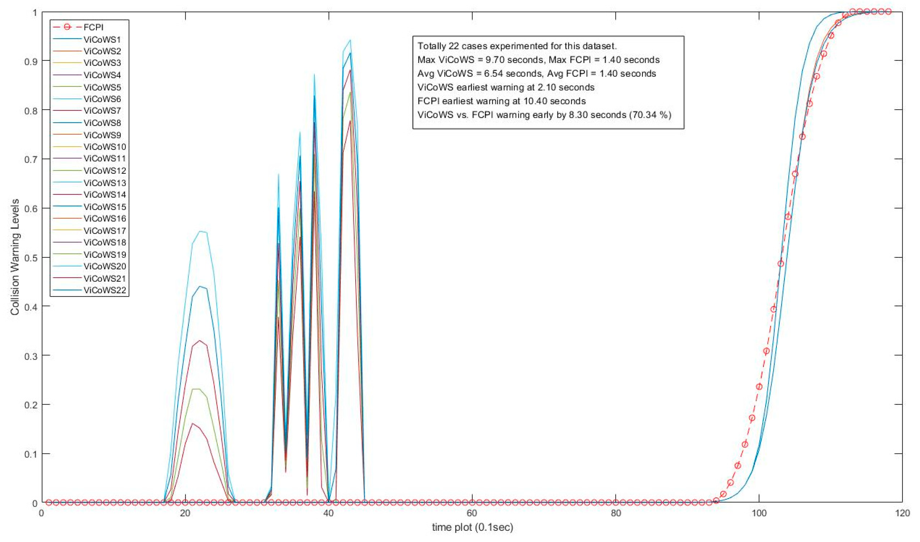
| C | 118 | 22 | 37~44 | 7.11~5.83 | 25~16 | 9.7 | 1.4 * | 8.3 | 70.34 |
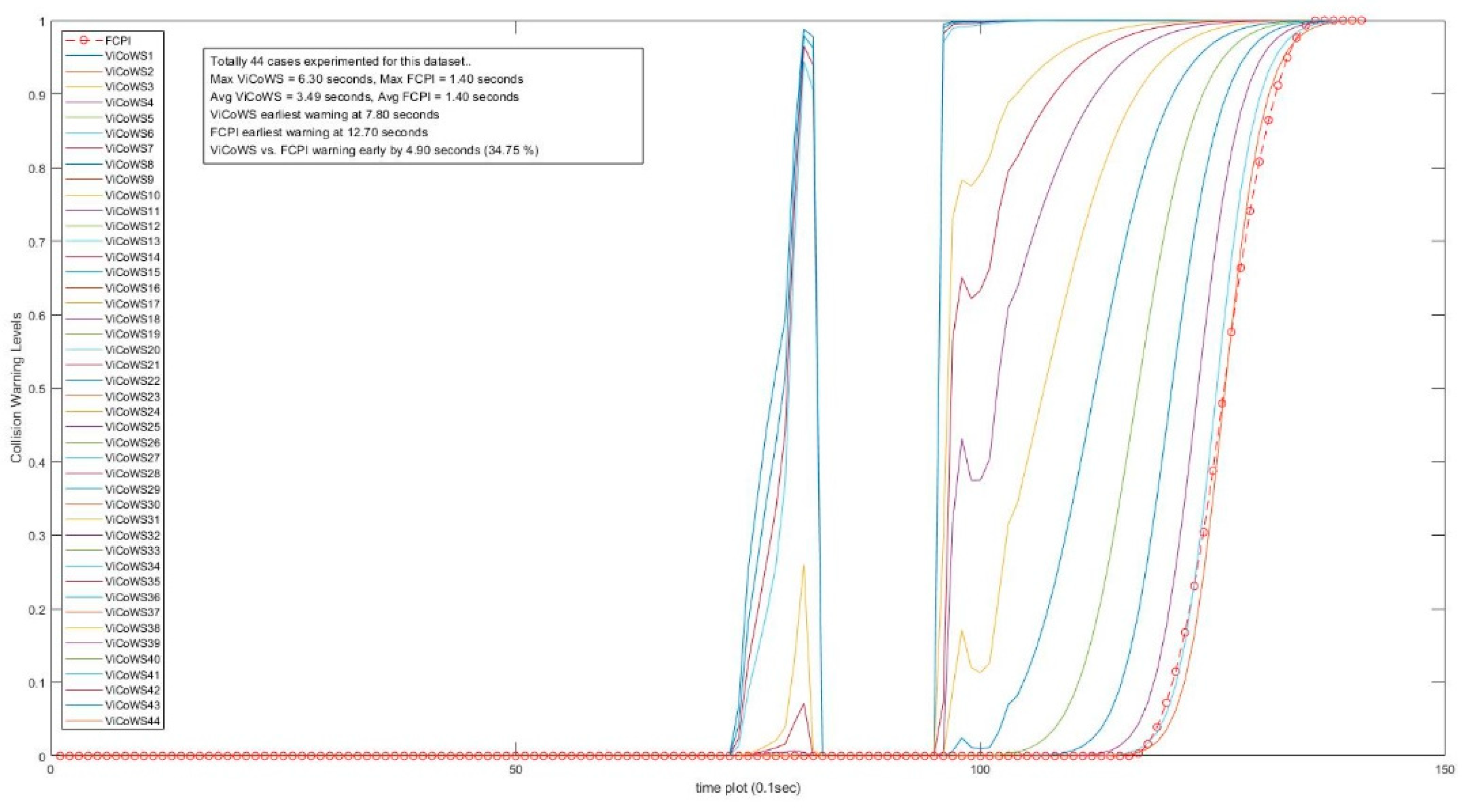
| D | 141 | 44 | 50~488 | 5.08~0.76 | 23~3 | 6.3 | 1.4 * | 4.9 | 34.75 |
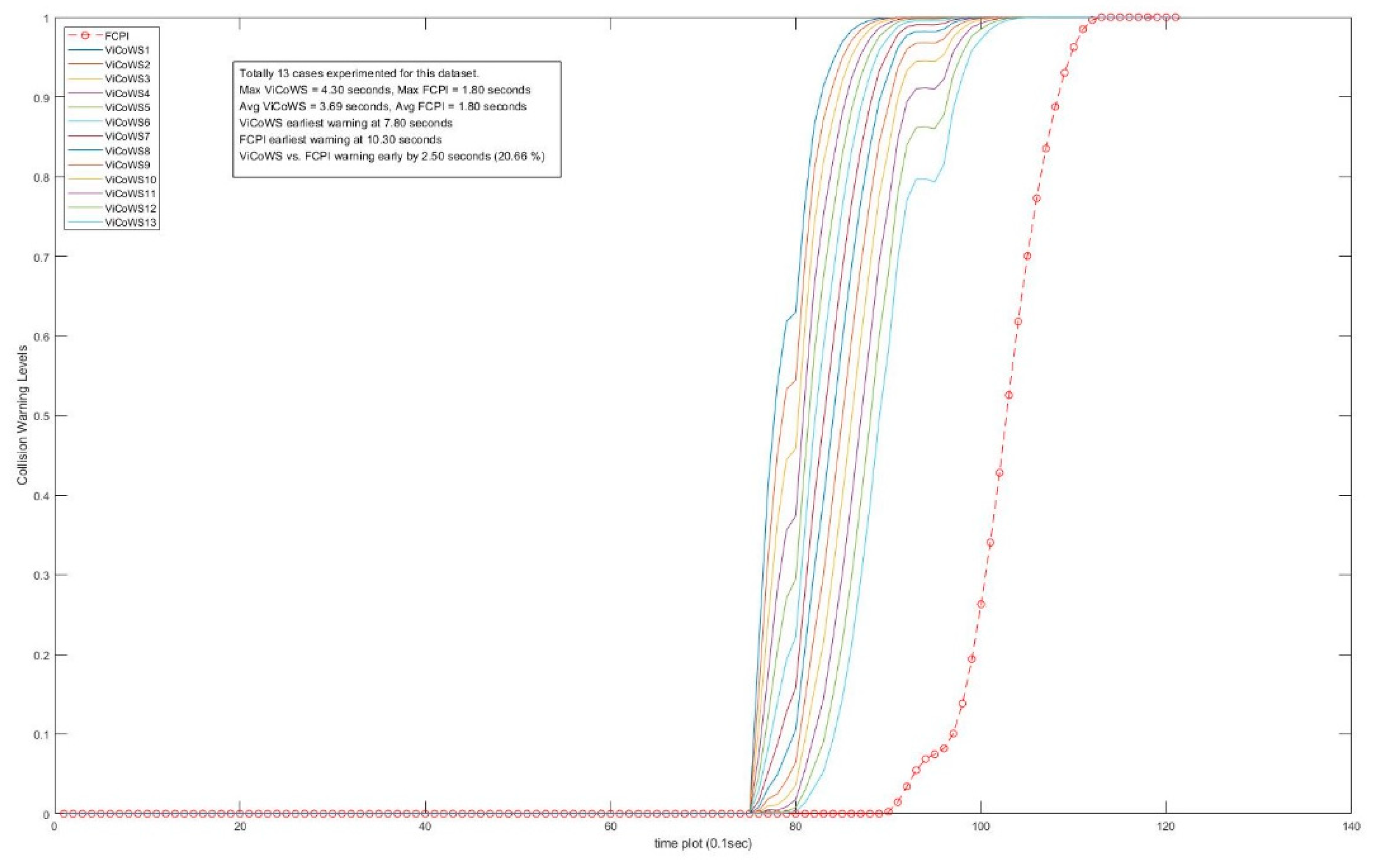
| E | 121 | 13 | 221~515 | 1.24~0.74 | 25~20 | 4.3 | 1.8 * | 2.5 | 20.66 |
| Total | 567 | 153 | Average Earlier by | 5.0 | 45.38 | ||||
© 2018 by the authors. Licensee MDPI, Basel, Switzerland. This article is an open access article distributed under the terms and conditions of the Creative Commons Attribution (CC BY) license (http://creativecommons.org/licenses/by/4.0/).
Share and Cite
Chen, K.-P.; Hsiung, P.-A. Vehicle Collision Prediction under Reduced Visibility Conditions. Sensors 2018, 18, 3026. https://doi.org/10.3390/s18093026
Chen K-P, Hsiung P-A. Vehicle Collision Prediction under Reduced Visibility Conditions. Sensors. 2018; 18(9):3026. https://doi.org/10.3390/s18093026
Chicago/Turabian StyleChen, Keng-Pin, and Pao-Ann Hsiung. 2018. "Vehicle Collision Prediction under Reduced Visibility Conditions" Sensors 18, no. 9: 3026. https://doi.org/10.3390/s18093026
APA StyleChen, K.-P., & Hsiung, P.-A. (2018). Vehicle Collision Prediction under Reduced Visibility Conditions. Sensors, 18(9), 3026. https://doi.org/10.3390/s18093026