Dynamic Toolface Estimation for Rotary Steerable Drilling System

1
College of Information and Control Engineering, China University of Petroleum, Qingdao 266580, China
2
School of Petroleum Engineering, China University of Petroleum, Qingdao 266580, China
*
Author to whom correspondence should be addressed.
Sensors 2018, 18(9), 2944; https://doi.org/10.3390/s18092944
Submission received: 16 July 2018
/
Revised: 24 August 2018
/
Accepted: 1 September 2018
/
Published: 4 September 2018
(This article belongs to the Special Issue Sensing in Oil and Gas Applications)
Abstract
:In drilling engineering, Toolface is an angle used to describe bit direction. It is a challenging task to accurately estimate Toolface while drilling because of the downhole harsh conditions, but it is a primary step for the dynamic point-the-bit rotary steerable system (DPRSS). A new dynamic Toolface estimator is present, which fuses measurements from two accelerometers and one gyro. A dual-accelerometer Toolface measuring method is designed to compensate the circumferential acceleration of DPRSS. A nonlinear Complementary Filter (CF) is used to suppress the effect of vibration and axial acceleration. The frequency-domain characteristics of nonlinear CF are analyzed and its natural frequency is determined adaptively based on real time drilling conditions. This new estimator is validated on a DPRSS prototype under typical drilling modes; it is demonstrated with high robustness and follows the references satisfactorily.
1. Introduction
Dynamic Point-the-bit Rotary Steerable System (DPRSS) is a novel drilling equipment or technology which builds a wellbore along a predefined trajectory quickly and dramatically reduces the drilling cost [1]. Comparing with the static rotary steerable system, DPRSS reduces friction resistance and reaches larger ultimate horizontal displacements [2]. The benefit of DPRSS mainly comes from its closed-loop control functions, and dynamic Toolface measurement is the primary step. However, the complex downhole drilling conditions, such as circumferential and axial vibration, and more specifically stick-slip, will result in additional measurement noise. There has been little discussion on dynamic Toolface estimation for DPRSS while drilling.
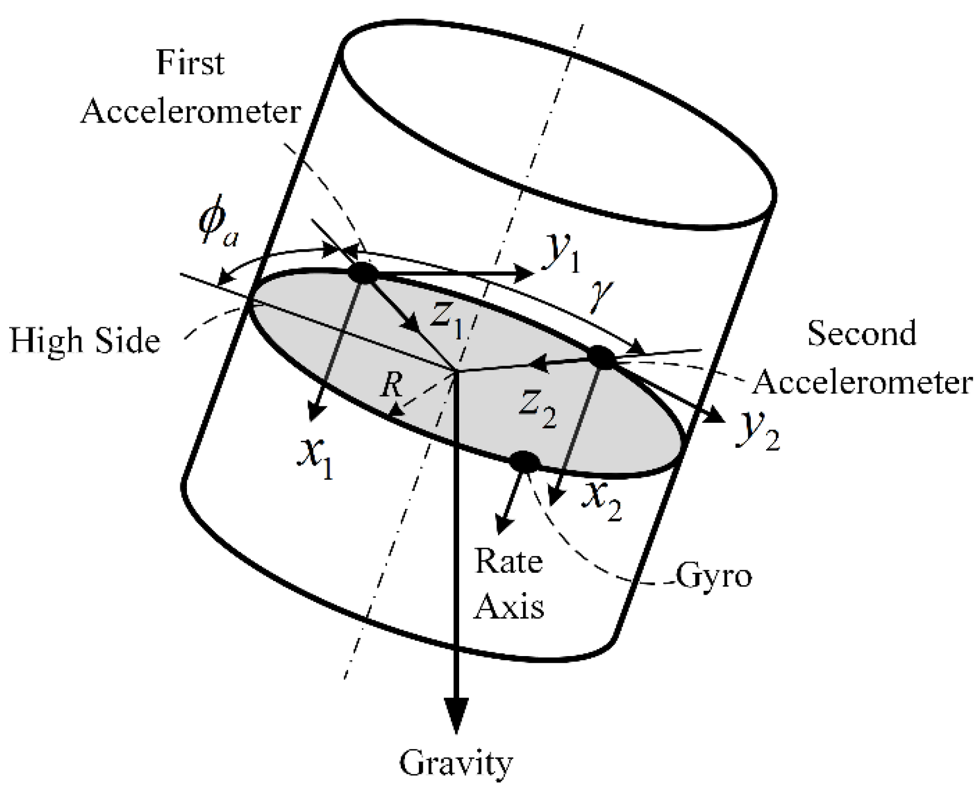
A DPRSS structure is shown schematically in Figure 1 [3,4]. The sleeve drilling torque and weight are imposed on the bit through a universal joint. A stabilized platform is assembled inside sleeve and driven by a motor; it has an eccentrically located receptacle which receives one end of the bit shaft. Sensors for Toolface measurement are installed on the surface of the stabilized platform. A left-handed coordinate system is defined in Figure 1, with the X-axis pointing to the bit, the Z-axis pointing to the center of the stabilized platform, and the Y-axis perpendicular to the XZ plane. In the YZ plane, the top of the borehole is named the high side, and the angle of the Z-axis clockwise relative to the high side is named the gravity Toolface, which is denoted by and is defined between 0 to 360 degrees. Toolface is used to describe bit direction, and it is controlled and adjusted by the stabilized platform.
In practice, there are three different ways to obtain Toolface. The first one is based on the tri-axial accelerometer [5,6], but in the drilling process, besides the kinematic motion acceleration, the drilling shock can be over 200 g [7] and the vibration acceleration is over 5 g [8,9]. Therefore, this method cannot provide an accurate Toolface estimation [5]. The second one is based on angular rate integration. The micro-electro-mechanical system (MEMS) gyro has been used because of its excellent vibration immunity. However, the MEMS gyro has relatively high nonlinearity, random walk and temperature drift due to its inherent drawbacks, and the drift of the MEMS gyro is up to 150°/h [10]. The third one is based on tri-axial magnetometers, such as flux gate. The magnetometers are free from vibration too. There is a theoretical relationship between the measurement results of gravitational accelerometer and magnetometer [11]. However, owing to the motor leakage flux in DPRSS, the operational envelope of magnetometers is limited. Hence, although the accelerometer and the gyro are selected and installed on the DPRSS stabilized platform, it is impossible to obtain an accurate Toolface estimation only through either of the two types of sensors.
There are three problems for the dynamic Toolface estimation. The first one is how to remove the effect of downhole vibration and the acceleration on the gravitational sensor. The second one is how to deal with the gyro drift errors, especially for high temperature applications. The third one is how to develop a high performance data fusion method, through which the strengths of the two types of sensors can be utilized and the gap between them can be bridged.
Based on these findings, a multi-sensor fusion algorithm has been considered. Two classes of multi-sensor fusion technologies are widely used in the measurement field. They are Kalman Filter (KF) and Complementary Filter (CF) [12]. Higgins [13] and Brown [14] illustrated the relationship between them. Higgins points out that CF is actually a steady-state KF. KF-based techniques have been studied in the areas of downhole inclination and azimuth estimation [6,15,16], but most of those methods are complex and impose high computational demand.
Besides the fact that CF is simple and efficient in attitude estimation in contrast with KF [12,17,18], two aspects have also been considered in our selection of CF, namely (1) the gyro measurement is immune to vibration while the accelerometer is sensitive to it; (2) the gyro drift and bias are low frequency signals while the vibration which affects the accelerometer is high frequency signals [19], and the two inertial sensors can complement each other in the frequency domain. Hence, it is possible for the most reliable frequency components of the two sensors measurement to be extracted through CF, and the key factor of CF designing is the selection of natural frequency for different dynamic conditions.
A new Toolface estimation method is proposed, which consists of a dual-accelerometer Toolface measurement and a nonlinear adaptive CF scheme. By analyzing the nonlinear CF frequency characteristics, a constant CF damping ratio was determined and only the CF natural frequency is to be designed. Moreover, the CF natural frequency is determined adaptively by a switch function. Several typical drilling modes were tested on a DPRSS prototype. Toolface estimation results were compared with a motor resolver angular position which is used as a reference in the laboratory. The Toolface estimator showed satisfactory performance in a DPRSS prototype, and future work will focus on its application in actual drilling operations.
This paper is organized as follows: Section 2 provides preliminary knowledge, which includes a short review of CF, Toolface estimation from tri-axial accelerometer and gyroscope. Section 3 shows a comprehensive explanation on the proposed Toolface estimator. Section 4 provides the test results. Section 5 is the conclusion and future work.
2. Preliminaries
2.1. Toolface Estimation from Tri-Axial Accelerometer
As shown in Figure 1, the tri-axial accelerometer is installed on the surface of the stabilized platform, where the radius is denoted by R. The tri-axial accelerometer X-axis, Y-axis and Z-axis measurements are denoted by , and , respectively. Toolface estimation from the accelerometer is denoted by which can be calculated as follows:
When the stabilized platform is rotated with an angular rate , the and are expressed in Equation (2):
where is the YZ plane gravity component, is the Toolface real value, and the two terms and are tangential and centripetal acceleration, which represent motion accelerations, and will make and different from their gravity components. The other two terms and represent additive measurement error arose from the vibration of the stabilized platform and the accelerometer measurement errors.
Considering the four additional terms, Toolface calculated from Equation (1) is different from its real value, the degree of deviation depending on the magnitude of the terms related to and . Additionally, the vibration acceleration is high frequency signals comparing with the variation of Toolface, and can be eliminated by a low-pass filter. However, the centripetal acceleration is a constant bias, which must be removed before using Equation (1).
2.2. Toolface Estimation from Gyro
The gyro is also installed on the surface of the stabilized platform, its rate axis parallel with the X-axis. The error model used in this paper is [20,21]:
where is the gyro measurement, is the stabilized platform angular rate, and is the low-frequency time-varying bias; denotes the additive measurement noise which is assumed to be white noise. The Toolface is obtained by:
where, is the gyro Toolface estimation, is the Toolface initial value, and denotes the gyro integration error from bias and measurement noise. It is clear that the accuracy of is affected by and .
2.3. Complementary Filter
CF is a distortionless filter or all pass filter [21] which is designed with a high pass filter (HPF) and a low pass filter (LPF). For Toolface estimation, CF combines high frequency components from and the low frequency components from . As such, true Toolface is obtained while noise is filtered as desired.
The basic structure of CF is shown in Figure 2. Let be the HPF transfer function and is the complementary LPF transfer function; the function of CF is given as:
For the noiseless measurement, the can be defined as a constant, i.e., , being the termed weighting factor. This type of CF is named linear CF [22] or first order CF [12], but it does not act as HPF or LPF.
In practice, CF is reconfigured to a control system scheme which is shown in Figure 3, where has the same meaning as a controller. In this case, CF is easy to implement and the classical controller design techniques can be used in filter design.
If is a proportional controller, i.e., , the function of CF is given by:
where s is the Laplace variable and the gain is cut-off frequency (rad/s). The error equation of Equation (6) is:
where is the final Toolface estimation error, is the gyro measurement error, and is the accelerometer measurement error. Applying the final value theorem to Equation (7),
In Equation (8), the final value of is not zero. In order to improve the performance of CF, a proportional-integral (PI) controller is introduced:
Then, the function of CF is given by:
where,
The is an HPF transfer function and is the complementary LPF transfer function. Applying the final value theorem to Equation (10):
The CF shown in Equation (10) is named the nonlinear CF, its estimation error converges to the accelerometer measurement error, and the gyro measurement error does not exist in Equation (12).
3. Toolface Estimation Method
3.1. Dual-Accelerometer Toolface Measurement
As previously mentioned in Section 2, the low frequency component of and the high frequency component of are fused by nonlinear CF, however, the motion acceleration of the stabilized platform has effects on low frequency component of . To remove this effect, a dual-accelerometer Toolface measurement method is proposed.
As shown in Figure 4, two accelerometers are installed on the surface of stabilized platform, the angle between two accelerometers is denoted by , the Y-axis and Z-axis measurements are as follows:
where the subscript 1 and 2 represent the first and the second accelerometer, respectively, while the other terms are the same as Equation (2). When the two accelerometers are oppositely placed, i.e., , the is equal to and is equal to , we can obtain:
where and are the processed measurements. The dual-accelerometer measurement method cannot be used to correct the X-axis measurement, which is denoted by , in the case of estimating downhole total acceleration, the average of and is used as . In Equation (14), the terms and , which represent the motion acceleration, are removed, while the YZ plane gravity component and the vibration acceleration terms and are magnified with same factor, so the Dual-accelerometer Toolface measurement can be calculated as the following:
It is clear that Toolface has a singularity at 360° [23]. In practice, and occur across 360° at a different time due to sensor measurement delay, thus, when an undesired large error arises, it reduces CF performance. To realize a full range accurate Toolface estimation, a preprocessing method is used which limits errors between −180° and 180°.
3.2. Toolface Adaptive Nonlinear CF Scheme
The CF performance is determined by and . Based on Equation (11) and the classical frequency design method [18], the mathematical relationship for and are given as Equation (17):
where is the natural frequency, rad/s; is the damping ratio. In order to simplify the CF parameter design, the damping ratio is selected as a constant, and the natural frequency is to be tuned for satisfactory CF performance.
3.2.1. Frequency-Domain Characteristics of Nonlinear CF
The and magnitude curves intersection is denoted by , is the intersection frequency and is the intersection magnitude. Let
One obtains:
The resonance points of and are denoted by and respectively. Let
Then one obtains,
From Equations (19) and (21), it can be seen that the magnitudes of the intersection point and resonance point are determined by , while the frequencies of the two points are related to and .
The nonlinear CF magnitude curves with different and are shown in Figure 5. In the first graph, is fixed, the filters’ magnitude curves are different from each other, and the magnitude of LPF and HPF depended on the value of . All of the intersection frequencies are larger than , and increase with . In the second graph, is fixed, the shape of magnitude curves is the same, but intersection frequencies are still larger than corresponding . CF noise suppressing performance is closely related with the magnitude curve, especially the curve shape in the vicinity of resonance frequency, which can be designed by selecting proper , and the trade-off between HPF and LPF can be realized by selecting .
In literature, is designed experimentally [18,24,25]. From Equations (19) and (21), it can be seen that when , the HPF do not have resonance due to only having imaginary solutions, and , which reveals that the LPF resonance cannot be removed.
Figure 6 presents the relationship between and , the is plotted in dB units. In this graph, and have a negative nonlinear correlation, while small can be obtained by increasing . However in Figure 5, large leads to a small roll-off rate, and the design of CF seeks to make the roll-off as narrow as possible. In this case, the CF performance will be close to its ideal design.
3.2.2. Adaptive Nonlinear CF Scheme
In order to make a narrow roll-rate and remove HPF resonance, is fixed to 0.707, thus, is fixed to 2.1 dB, then, the CF is only characterized by . A larger means a more high frequency component of sensors will be included in Toolface estimation of CF output, hence, a better dynamic response is obtained, while a smaller means the high frequency components of sensors will be filtered, and Toolface estimation will steadily follow the major trends of real Toolface.
Various types of CF parameter designing method have been proposed. A fixed weight factor is implemented in linear CF [12], but the fixed gains cannot converge properly under complex circumstances. While neglecting any motion accelerations, the error e which is shown in Figure 3 is used as a cost-function, then intelligence stochastic searching algorithm [22] and the least square error method [26] are introduced to obtain optimal and . Gain-scheduled CF is introduced [18], the gains are selected from three predetermined values and switched discontinuously. To improve CF performance, the gain-scheduling rules must contain more scenarios and be fine-tuned. The fuzzy logic based CF gain switch logic is commonly adopted [24,25,27,28] to continuously switch gains based on error levels, but it leads to increased computational time, as the fuzzy logic parameters tuning is a complex task.
The dynamic intensity was usually described by absolute acceleration magnitude, by which the switch function is designed [18,25,27], but in the drilling process, the additional acceleration is strong and always exists, the absolute acceleration magnitude are most likely to lead to incorrect CF gain switches.
Due to the acceleration magnitude being positively correlated with vibration severity, the variance of acceleration magnitude is used as the vibration factor in calculation:
where is the variance of the acceleration magnitude. Similarly, the variance of rotation rate denoted by is another factor in calculation. In practice, the and are calculated by rolling variance, they are updated during each sampling period.
The dynamic intensity is described by , where the m and n are two weight factors of vibration and angular rate. Based on the rules designed by Hong [18], the general gain-schedule rule is shown in Figure 7, the dynamic intensity is separated into several levels, and the best for each levels is determined by experimental data and off-line optimization [29].
In Figure 7, as the dynamic intensity increases, the difference of between two dynamic intensity levels becomes small. Obviously, the exponential function is a good selection to fit or approximate the relationship between and dynamic intensity, so the switch function is designed as follows:
where is the maximum of , rad/s. It should be noted that the switch function is not unique, but the Equation (23) is simple and shows satisfactory performance during our experimental tests. The CF natural frequency can be determined based on the dynamic intensity adaptively and continuously.
There are two methods to design : (1) can be set to be equal to when vibration and motion acceleration are relatively low; (2) low frequency information can be obtained by Fast Fourier Transformation analysis, then we can define the passband of , and can be slightly larger than the passband. According to Zhou and Liu [30,31], when the low-pass filter cut-off frequency is less than 0.2 Hz, the vibration acceleration affections can be eliminated, after analyzing several frequency magnitude curves, we choose to be 0.3 rad/s (0.05 Hz).
The two weight factors m and n define how fast does change regarding the vibration and angular rate. Due to most of the motion acceleration effect being complemented by the dual-accelerometer measurement method, vibration is the key factor to be considered in the CF scheme. A simple way to tune m and n is: Setting n to 0 at the beginning of parameter tuning, then m can be tuned, after that, increasing n slowly until Toolface estimation satisfies the accuracy requirements. In this way, m and n might not be optimal, but it is easy to carry out the tuning in practice.
The proposed dynamic Toolface estimation nonlinear CF scheme is shown in Figure 8. The figure denotes estimated initial Toolface as , then can be calculated:
Dynamic Toolface is obtained in the following steps:
- Step 1:
- Initialization: Acquire data from dual-accelerometer in steady state, calculate by Equation (15), let and ;
- Step 2:
- Start estimation: Calculate and by Equation (15) and Equation (16), respectively;
- Step 3:
- Calculate and by Equation (22), then obtain from Equation (23);
- Step 4:
- Calculate by Equation (24), GOTO step 2 for next instant.
4. Experiments and Results
4.1. DPRSS Prototype for Experiments
As shown in Figure 9, a DPRSS prototype is developed. The sleeve is horizontally placed on a fixed stand. The stabilized platform, which is driven by motor, is assembled inside the sleeve. Two MMA8451 accelerometers and an HTG-1200 gyro are mounted on a stabilized platform in the manner shown in Figure 4, where R = 0.025 m, and the sensors specifications are shown in Table 1. A 16-bit AD converter ADS8320 is used to acquire the output of gyro. An MC9S12XS128 microprocessor is attached to the accelerometers and AD converter via serial communication. A resolver which can measure motor rotor position and angular rate is installed at the end of the motor, a 14-bit R/D converter is used to convert the resolver analog output to a digital signal. A TMS320F28335 DSP is attached to the R/D converter via SPI communication, and the DSP is also used to control the motor velocity and rotor position. All data were acquired via USB-CAN analyzer with a 200 Hz sample rate and processed by Matlab software. During the experiment, the sleeve was non-rotational, and the motor rotor position denoted by was considered to be the Toolface reference, the root mean square error (RMSE) of estimation results was selected as an index of CF performance.
4.2. Dual-Accelerometer Toolface Measurement Test
The references, raw accelerometer output and dual-Toolface measurement results are shown in Figure 10. The stabilized platform angular rate was switched based on a square wave.
The stabilized platform setting angular rate was ±900°/s, it was a straight forward process to calculate that the maximum tangential acceleration and centripetal acceleration were 2.7 g and 0.638 g, respectively. In Figure 10, the Y-axis maximum difference between the single accelerometer and the dual-accelerometer measurement is 2.8 g and the Z-axis maximum value is 0.628 g, which is in accordance with theoretical analysis, while the motion acceleration is suppressed. The RMSE of the single accelerometer and dual accelerometer are 52.7° and 24.9°, respectively. It should be noted that though a nearly motion-free measurement has been obtained, the vibration effect still needs to be considered.
4.3. Dynamic Toolface Estimator Performance Test
The DPRSS prototype is placed horizontally and firmly fastened to a vibration platform. The vibration platform generates vertical vibration with variance frequency of between 0 and 50 Hz. In the test, and which are shown in Equation (22) are calculated by rolling variance, a small relative rolling window size shows more details while a relative large rolling window size shows more major trends, after trying various length of rolling windows, the window size is set to 10. In future research, the length of rolling windows should be adjusted according to the frequency properties of and .
The stick-slip phenomenon commonly exists in the drilling process, it is a mode of torsional vibrations of a drilling assembly, and its vibration baseband is less than 0.5 Hz [8,9]. Toolface variation rang is less than 20° in DPRSS porotype, a sine curve with 20° magnitude and 0.5 Hz frequency was designed to simulate the stick-slip vibration.
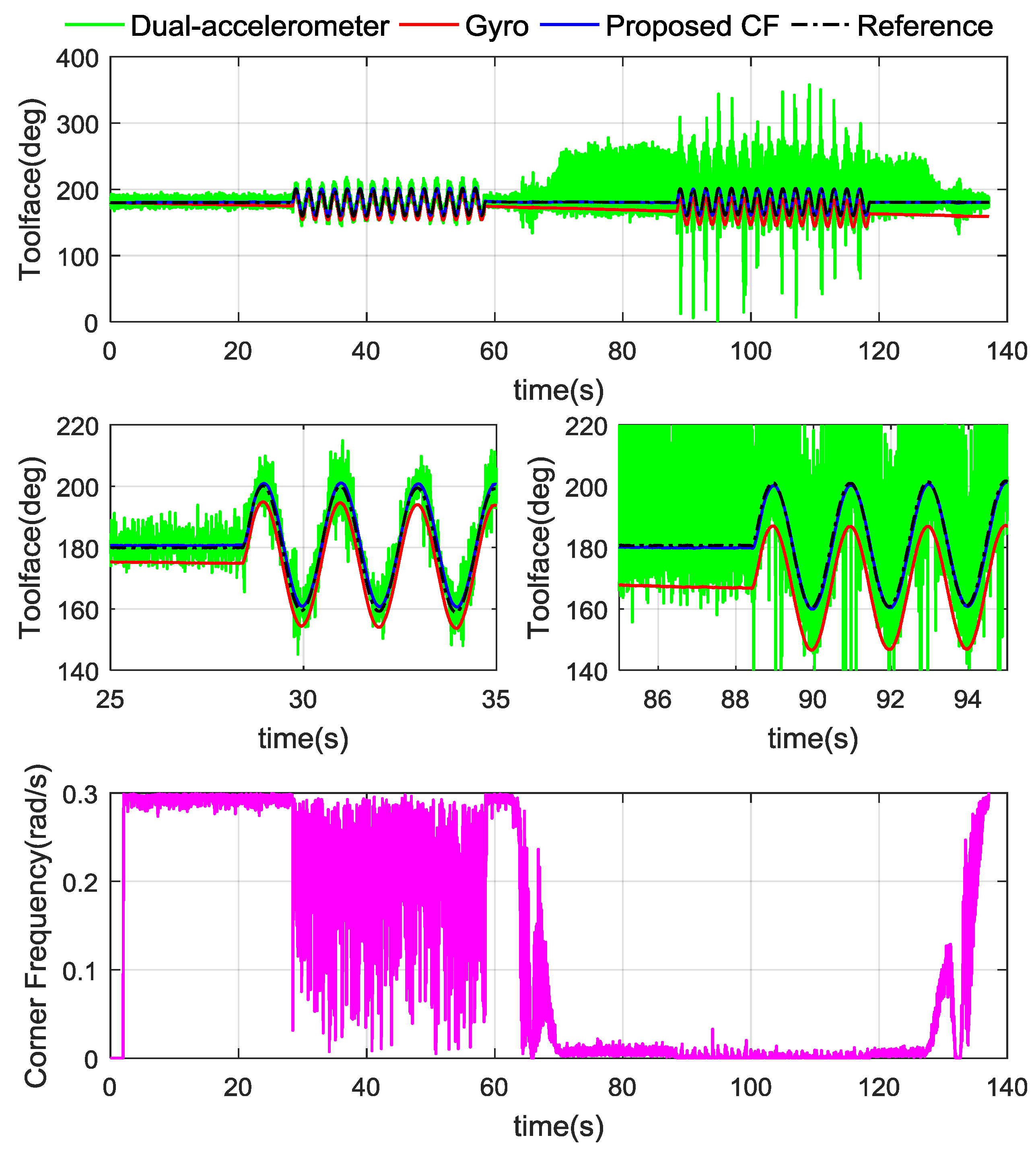
4.3.1. Stick-Slip Dynamic Toolface Estimator Test and Parameters Tuning
The tests were designed consisting of steady state and stick-slip state, while both non-vibration and vibration conditions were considered. There are four successive states: The first one is non-vibration and non-stick-slip, the second one is non-vibration and stick-slip, the following one is vibration and non-stick-slip, the last one is vibration and stick-slip.
The dual-accelerometer Y-axis and Z-axis measurements are depicted in Figure 11. During the experiment, was 0.3 rad/s, m was selected between 0 to 50 with equal intervals, n was selected in the same way, the raw sensor data in Figure 11 was used for testing. By carrying out rigorous sets of experiment with different parameters, the effect of m and n values on Toolface estimation performance was studied.
In Figure 12, RMSE of dynamic Toolface estimator varies with the selection of different m and n, but they are all less than 8.2°, whereas over 82% of the RMSE values are less than 4°. When m = 12.12 and n = 45.96, the least RMSE is obtained. In fact, due to m and n only changing the increase or decrease rate of for specific vibration and motion acceleration, these parameters do not have a significant impact on CF performance, as the adaptive CF scheme provides robustness against different m and n values.
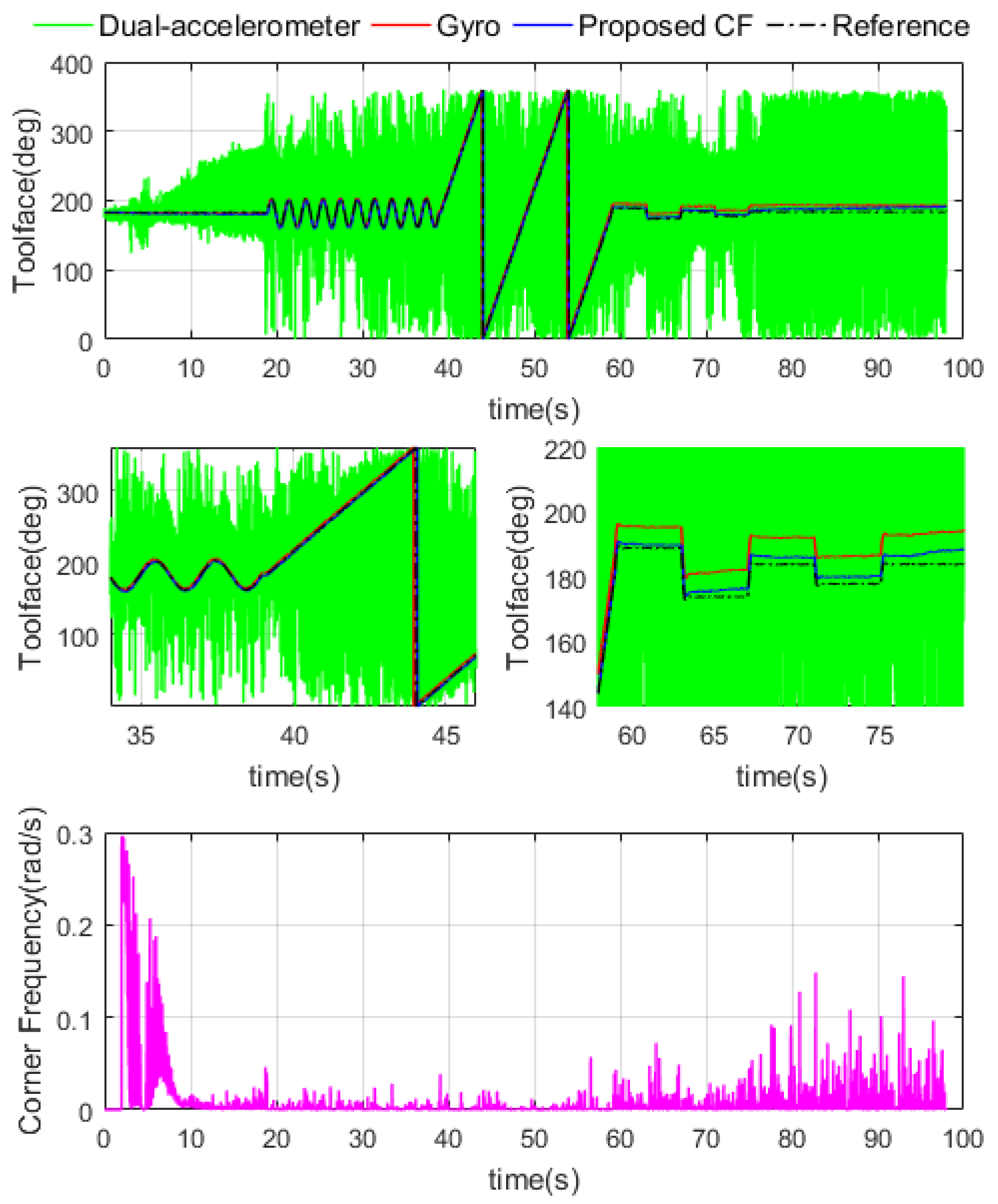
Let , the Toolface estimation results are shown in Figure 13. To initialize CF, of the first 2 s was 0 rad/s. It can be seen that follows the reference steadily, but has gradual instability of integration drifting. The CF natural frequency is switched as desired, more is used in the low acceleration state and more is used under high vibrations. By fusing and with the proposed CF scheme, trends to follow satisfactorily. According to Table 2, the RMSE of proposed CF scheme is 1.0069°, which is improved major improvement over the other two methods.
4.3.2. Multi Processes Dynamic Toolface Estimator Test
Four typical processes were designed to test the performance of dynamic Toolface estimator. Firstly, steady state, where the stabilized platform was non-rotational. Next is stick-slip. Thirdly, the stabilized platform rotated continuously, which was used to test full rang estimator performance. Finally, the stabilized platform was turned to different Toolface values, which is named the Toolface orientation drilling process. Dual-accelerometer measurements are shown in Figure 14, vibration effect and stick-slip motion effect can be observed.
The same parameters as Section 4.3.1 are used in this test, the performance of a well-designed estimator under different dynamic conditions was shown in Figure 15. Toolface from dual-accelerometer measurement, gyro and proposed estimator are plotted together. It is clear that dual-accelerometer measurement is affected by vibration, the gyro estimation is accurate at the beginning but shows gradual instability of integration drifting, and the proposed estimator shows promising performance in full range. The CF natural frequency values are shown in the fourth graph of Figure 15. Due to high dynamic intensity, the CF natural frequency remains relatively small, and more high frequency gyro components are used in CF results.
The RMSE of different Toolface results are demonstrated in Table 3, the robustness of the proposed CF under multi-drilling processes with vibration was shown. The data leads us to the conclusion that a well-designed Toolface estimator can offer a satisfactory performance. The proposed method could be usefully employed in actual DPRSS dynamic Toolface estimation.
5. Conclusions
The dynamic Toolface estimation is a key aspect of DPRSS. The complex drilling vibration and motion acceleration seriously affect the accuracy of Toolface measurement. A new dynamic Toolface estimator is proposed which is based on the measurements from two accelerometers and one gyro. A dual-accelerometer Toolface measurement method is used for complementing motion acceleration efficiently. An adaptive nonlinear CF scheme is used for fusing accelerometer and gyro measurements, the nonlinear CF damping ratio is fixed to 0.707, and its natural frequency is adaptively determined by an exponential function, and the function is correlated with dynamic intensity.
The performance of the estimator in several typical drilling modes were tested on a DPRSS prototype, the results indicate that the dual-accelerometer combined with the adaptive nonlinear CF is an efficient Toolface estimator for drilling engineering. The estimator extracts the most reliable components from the gyro and accelerometers, and provides a general and effective signal processing algorithm for downhole data. Future work would involve using the Dynamic Toolface estimator performance test in an actual drilling process.
Author Contributions
Conceptualization, W.W. and Y.G.; Methodology, W.W.; Software, K.W.; Validation, W.W. and K.W.; Formal Analysis, W.W. and J.S.; Investigation, K.W.; Resources, Y.G.; Data Curation, Y.G.; Writing-Original Draft Preparation, W.W.; Writing-Review & Editing, Y.G. and J.d.O.F.; Visualization, W.W.; Supervision, Y.G.; Project Administration, Y.G.; Funding Acquisition, Y.G.
Funding
This research was funded by [Ministry of Science and Technology of the People’s Republic of China] grant number [2016YFC0302800] and [Ministry of Education of the People’s Republic of China] grant number [15CX06065A] and [15CX08014A].
Conflicts of Interest
The authors declare no conflict of interest.
References
- Schaaf, S.; Mallary, C.; Pafitis, D. Point-the-bit rotary steerable system: Theory and field results. In Proceedings of the SPE Annual Technical Conference and Exhibition, Dallas, TX, USA, 1–4 October 2000; Society of Petroleum Engineers: Richardson, TX, USA, 2000. [Google Scholar]
- Zhang, C.; Zou, W.; Cheng, N. Overview of rotary steerable system and its control methods. In Proceedings of the 2016 IEEE International Conference on Mechatronics and Automation (ICMA), Harbin, China, 7–10 August 2016; pp. 1559–1565. [Google Scholar]
- Yan, Z.D.; Geng, Y.F.; Wang, Z.F.; Wang, W.L. Design of Offsetting Steerable Mechanism for Rotary Steerable Drilling Tool Based on Double Eccentric Rings. Appl. Mech. Mater. 2013, 288, 13–18. [Google Scholar] [CrossRef]
- Wang, W.; Geng, Y.; Yan, Z. Dynamic Point-The-Bit Rotary Steerable Drilling Tool and Measuring Method Thereof. U.S. Patent 9,587,440, 7 March 2017. [Google Scholar]
- Qilong, X.; Ruihe, W.; Feng, S.; Leilei, H.; Laiju, H. Continuous measurement-while-drilling utilizing strap-down multi-model surveying system. IEEE Trans. Instrum. Meas. 2014, 63, 650–657. [Google Scholar] [CrossRef]
- Elgizawy, M.; Noureldin, A.M.; El-Sheimy, N. Continuous wellbore surveying while drilling utilizing MEMS gyroscopes based on Kalman filtering. In Proceedings of the SPE Annual Technical Conference and Exhibition, Florence, Italy, 19–22 September 2010; Society of Petroleum Engineers: Richardson, TX, USA, 2010. [Google Scholar]
- Heinisch, D.; Oueslati, H.; Popp, T.M.; Meyer-Heye, B.; Schepelmann, C.; Reckmann, H. Testing and Characterization of Shock and Vibration Loads to Enhance Drilling Tool Reliability and Efficiency. In Proceedings of the Abu Dhabi International Petroleum Exhibition & Conference, Abu Dhabi, UAE, 7–10 November 2016; Society of Petroleum Engineers: Richardson, TX, USA, 2016. [Google Scholar]
- Ledgerwood, L.W.; Hoffmann, O.J.-M.; Jain, J.R.; El Hakam, C.; Herbig, C.; Spencer, R. Downhole vibration measurement, monitoring, and modeling reveal stick/slip as a primary cause of PDC-bit damage in today. In Proceedings of the SPE Annual Technical Conference and Exhibition, Florence, Italy, 19–22 September 2010; Society of Petroleum Engineers: Richardson, TX, USA, 2010. [Google Scholar]
- Sugiura, J. The use of the near-bit vibration sensor while drilling lead to optimized rotary-steerable drilling in push-and point-the-bit configurations. In Proceedings of the SPE Asia Pacific Oil and Gas Conference and Exhibition, Perth, Australia, 20–22 October 2008; Society of Petroleum Engineers: Richardson, TX, USA, 2008. [Google Scholar]
- ADXRS645 Datasheet. Available online: http://www.analog.com/media/en/technical-documentation/data-sheets/ADXRS645.pdf (accessed on 4 September 2018).
- Yang, Q.J.; Zuo, X.; Lin, E.H. A New Method for Dynamic Position Measurement While Drilling String Rotating. Appl. Mech. Mater. 2012, 152–154, 1102–1105. [Google Scholar] [CrossRef]
- Wu, J.; Zhou, Z.; Chen, J.; Fourati, H.; Li, R. Fast Complementary Filter for Attitude Estimation Using Low-Cost MARG Sensors. IEEE Sens. J. 2016, 16, 6997–7007. [Google Scholar] [CrossRef]
- Higgins, W. A Comparison of Complementary and Kalman Filtering. IEEE Trans. Aerosp. Electron. Syst. 1975, AES-11, 321–325. [Google Scholar] [CrossRef]
- Brown, R.G. Integrated navigation systems and Kalman filtering: A perspective. Navigation 1972, 19, 355–362. [Google Scholar] [CrossRef]
- Xue, Q.; Leung, H.; Wang, R.; Liu, B.; Wu, Y. Continuous Real-Time Measurement of Drilling Trajectory with New State-Space Models of Kalman Filter. IEEE Trans. Instrum. Meas. 2016, 65, 144–154. [Google Scholar] [CrossRef]
- Chao, D.; El-Sheimy, N. Continuous Measurement-While-Drilling Surveying System Utilizing Low-Cost SINS. In Proceedings of the SPE/IADC Middle East Drilling Technology Conference and Exhibition, Abu Dhabi, UAE, 26–28 January 2016; Society of Petroleum Engineers: Richardson, TX, USA, 2016. [Google Scholar]
- Benziane, L.; El Hadri, A.; Seba, A.; Benallegue, A.; Chitour, Y. Attitude Estimation and Control Using Linearlike Complementary Filters: Theory and Experiment. IEEE Trans. Control Syst. Technol. 2016, 24, 2133–2140. [Google Scholar] [CrossRef]
- Yoo, T.S.; Hong, S.K.; Yoon, H.M.; Park, S. Gain-scheduled complementary filter design for a MEMS based attitude and heading reference system. Sensors 2011, 11, 3816–3830. [Google Scholar] [CrossRef] [PubMed]
- Close, D.; Owens, S.; Macpherson, J. Measurement of BHA vibration using MWD. In Proceedings of the SPE/IADC Drilling Conference, Dallas, TX, USA, 28 February–2 March 1988; Society of Petroleum Engineers: Richardson, TX, USA, 1988. [Google Scholar]
- Tian, Y.; Wei, H.; Tan, J. An Adaptive-Gain Complementary Filter for Real-Time Human Motion Tracking with MARG Sensors in Free-Living Environments. IEEE Trans. Neural Syst. Rehabil. Eng. 2013, 21, 254–264. [Google Scholar] [CrossRef] [PubMed]
- Mahony, R.; Hamel, T.; Pflimlin, J.-M. Nonlinear Complementary Filters on the Special Orthogonal Group. IEEE Trans. Autom. Control 2008, 53, 1203–1218. [Google Scholar] [CrossRef] [Green Version]
- Poddar, S.; Narkhede, P.; Kumar, V.; Kumar, A. PSO Aided Adaptive Complementary Filter for Attitude Estimation. J. Intell. Robot. Syst. 2017, 87, 531–543. [Google Scholar] [CrossRef]
- Safa, A.; Baradarannia, M.; Kharrati, H.; Khanmohammadi, S. Global attitude stabilization of rigid spacecraft with unknown input delay. Nonlinear Dyn. 2015, 82, 1623–1640. [Google Scholar] [CrossRef]
- Hong, S.K. Fuzzy logic based closed-loop strapdown attitude system for unmanned aerial vehicle (UAV). Sens. Actuators Phys. 2003, 107, 109–118. [Google Scholar] [CrossRef]
- Shen, X.; Yao, M.; Jia, W.; Yuan, D. Adaptive complementary filter using fuzzy logic and simultaneous perturbation stochastic approximation algorithm. Measurement 2012, 45, 1257–1265. [Google Scholar] [CrossRef]
- Narkhede, P.; Joseph Raj, A.N.; Kumar, V.; Karar, V.; Poddar, S. Least square estimation-based adaptive complimentary filter for attitude estimation. Trans. Inst. Meas. Control 2018. [Google Scholar] [CrossRef]
- Duong, D.Q.; Sun, J.; Nguyen, T.P.; Luo, L. Attitude estimation by using MEMS IMU with Fuzzy Tuned Complementary Filter. In Proceedings of the IEEE International Conference on Electronic Information and Communication Technology (ICEICT), Harbin, China, 20–22 August 2016; pp. 372–378. [Google Scholar]
- Kang, C.H.; Park, C.G.; Song, J.W. An Adaptive Complementary Kalman Filter Using Fuzzy Logic for a Hybrid Head Tracker System. IEEE Trans. Instrum. Meas. 2016, 65, 2163–2173. [Google Scholar] [CrossRef]
- Jieru, S. Research on Measurement Method of Dynamic Point-the-Bit Rotary Steerable Drilling Tool; China University of Petroleum (East China): Qingdao, China, 2018. (In Chinese) [Google Scholar]
- Jing, Z.; Yi, Z.; Xing, L.; XIao, C.; Yingjun, J. Method of Eliminating Vibrational Acceleration in Rotary Steerable Drilling System. Oil Drill. Prod. Technol. 2010, 32, 19–22. (In Chinese) [Google Scholar]
- Baiyan, L.; Yi nao, S.; Xinyuan, C.; Jiangang, X.; Liangcai, Z. Theoretical and experimental investigation on dynamic measurements of hole inclination in automatic vertical drilling process. Acta Pet. Sin. 2006, 27, 105. (In Chinese) [Google Scholar]
Figure 1.
Schematic structure of DPRSS.
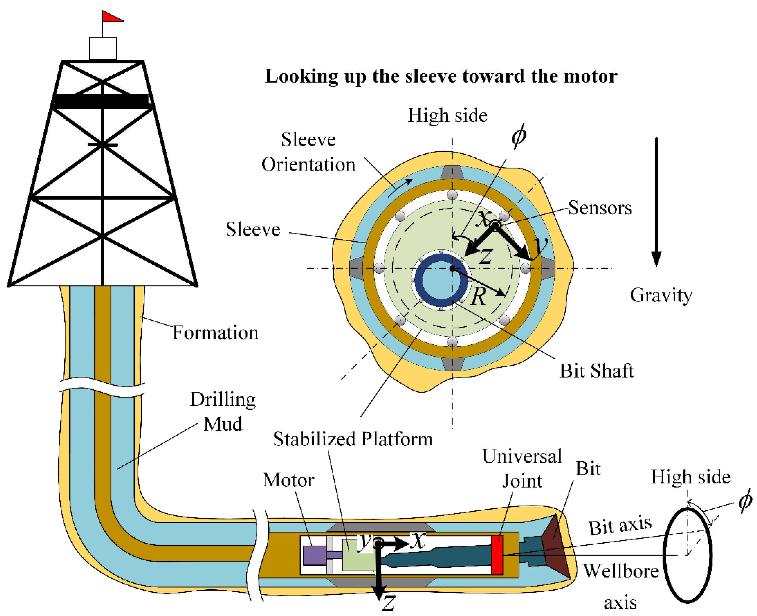
Figure 2.
Basic Structure of CF.

Figure 3.
Block diagram of basic CF.
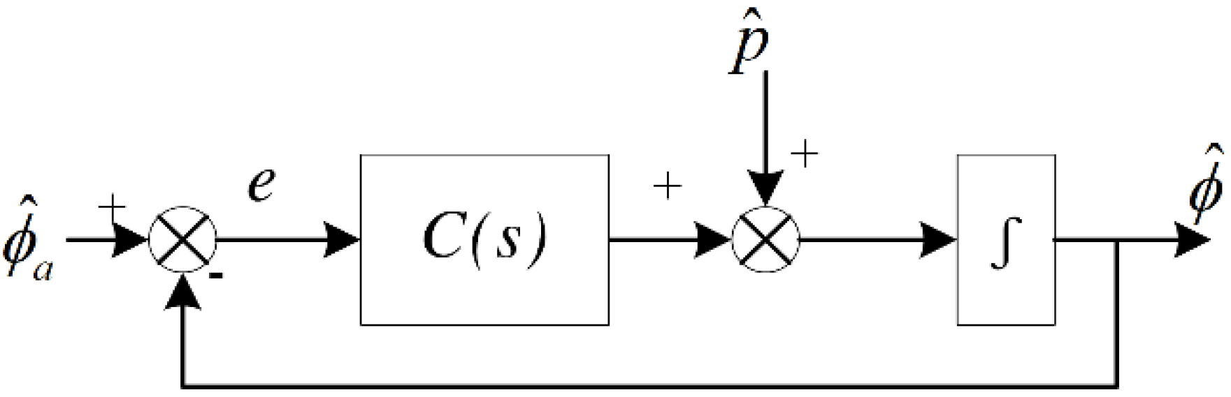
Figure 4.
Schematic diagram of dual-accelerometer Toolface calculation.

Figure 5.
Magnitude diagram of complementary filter.
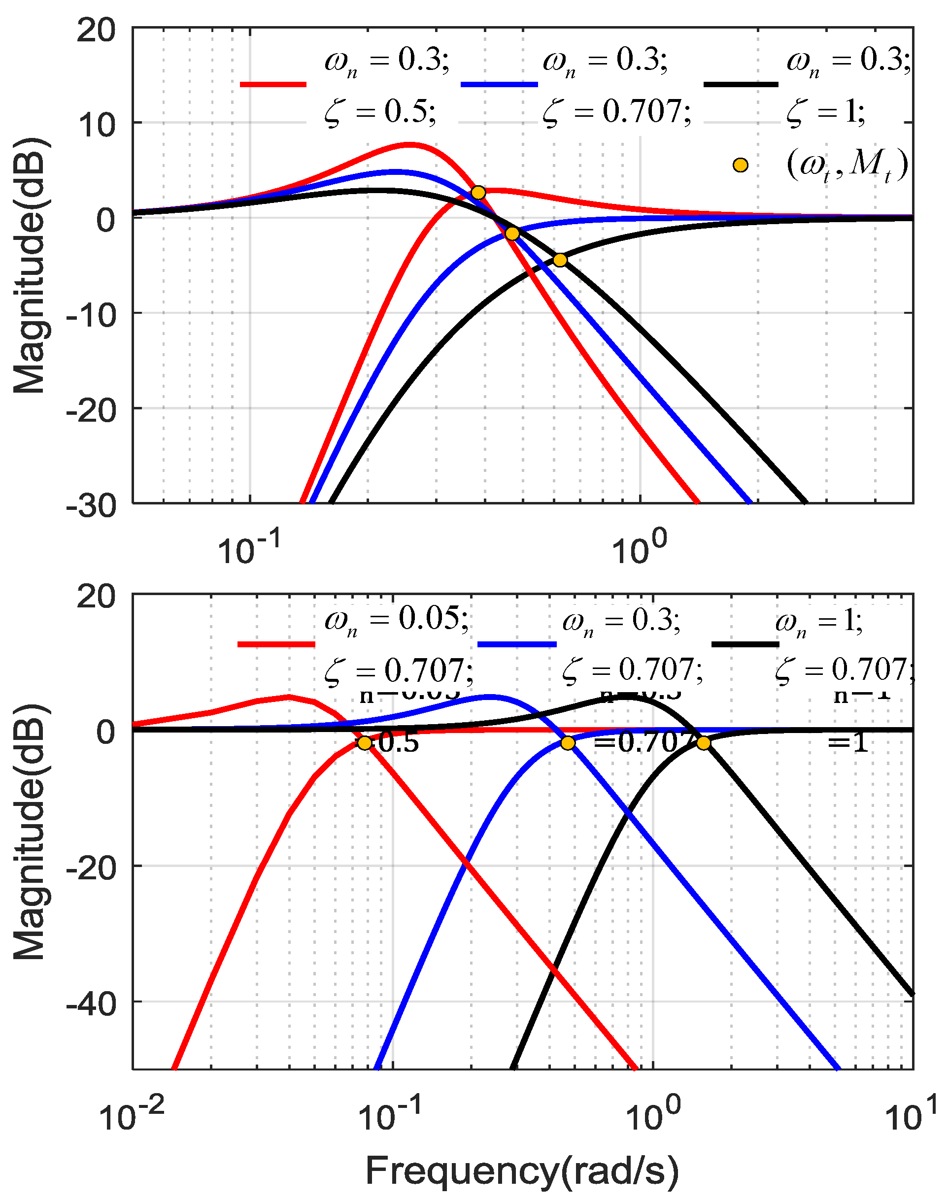
Figure 6.
Relationship between LPF Resonance Magnitude and CF Damping Ratio.

Figure 7.
CF gain-scheduling rules.
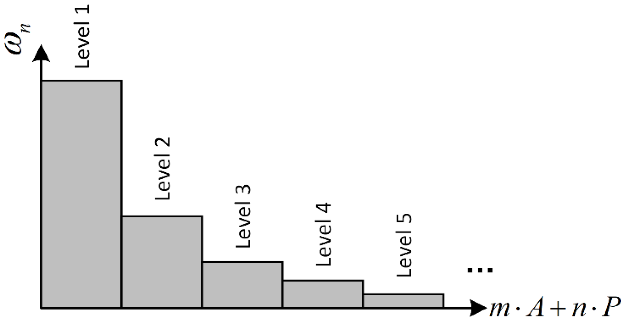
Figure 8.
Block diagram for proposed adaptive nonlinear CF scheme.

Figure 9.
DPRSS Prototype.
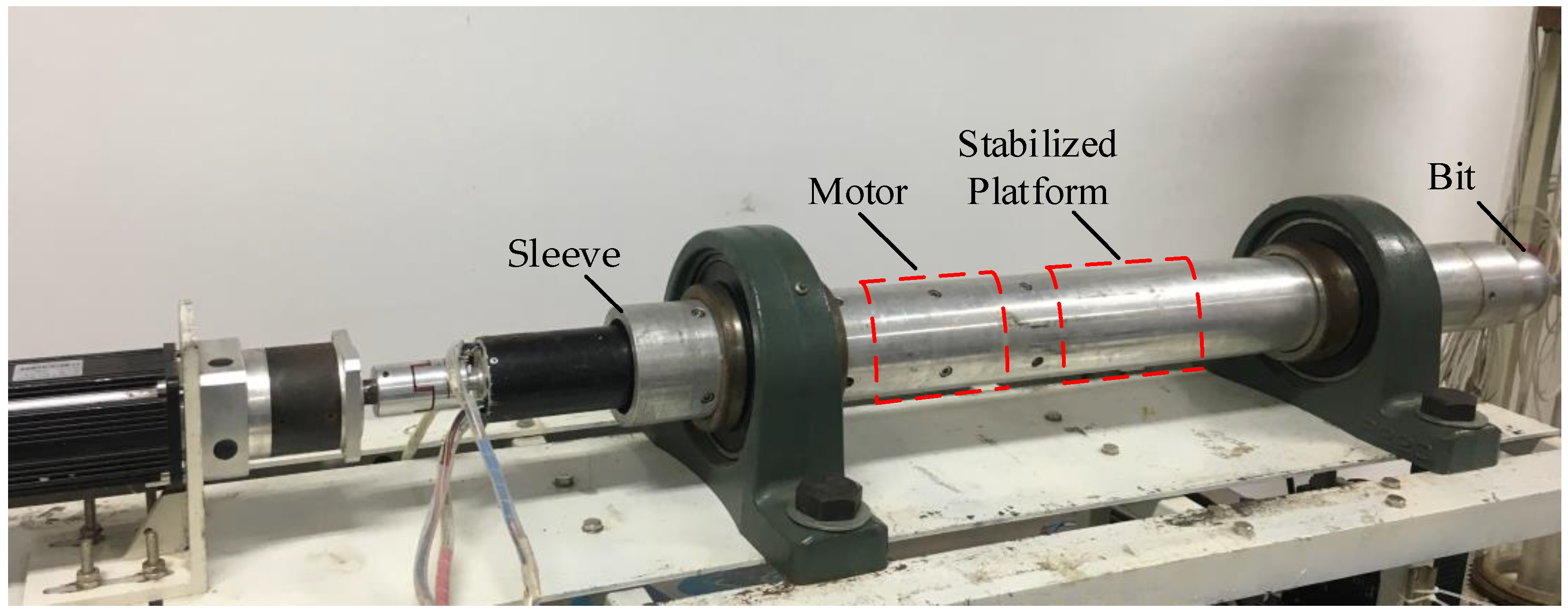
Figure 10.
Stabilized platform angular rate, raw accelerometer data, and Toolface comparison.
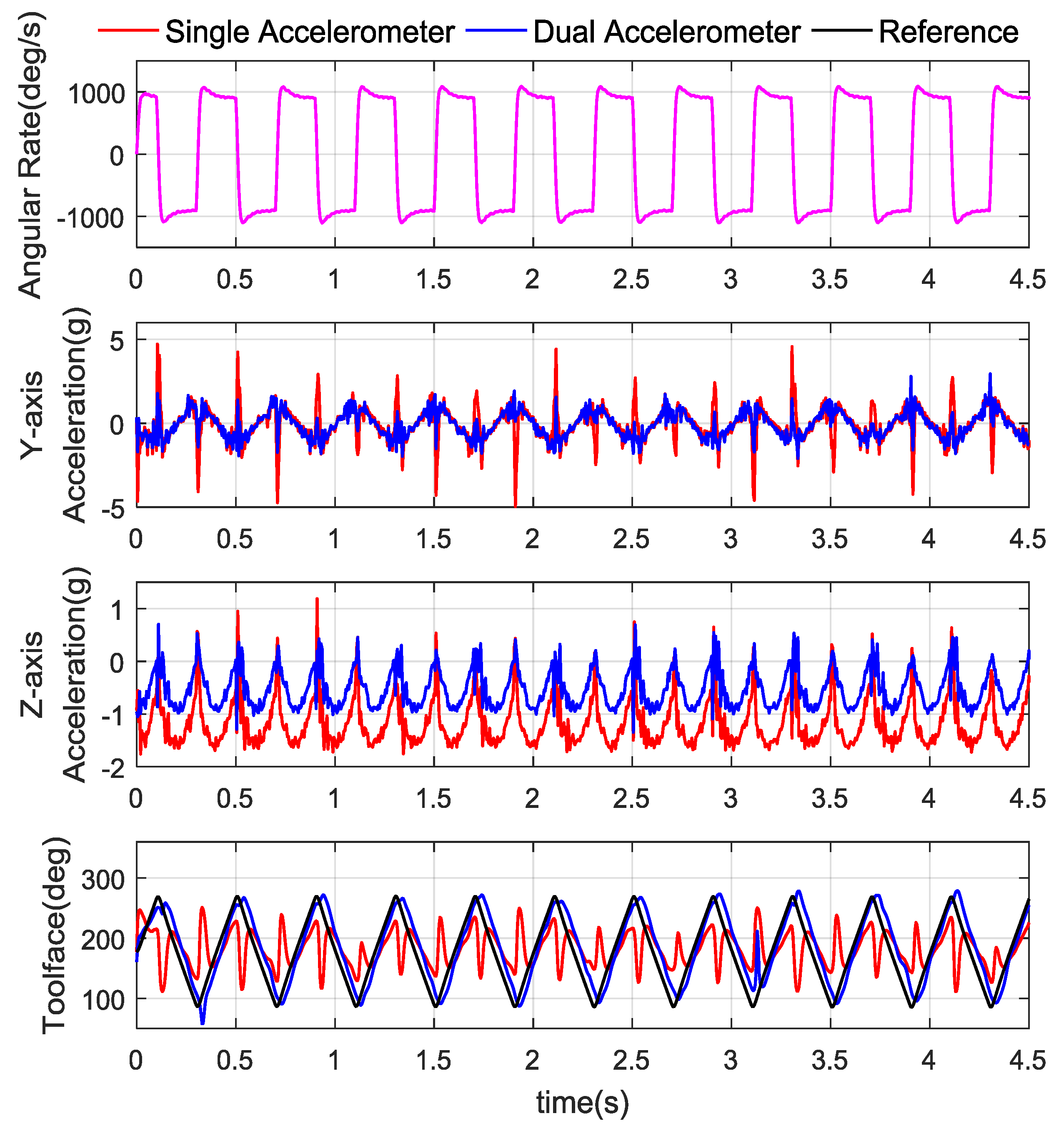
Figure 11.
Y and Z axis measurements.
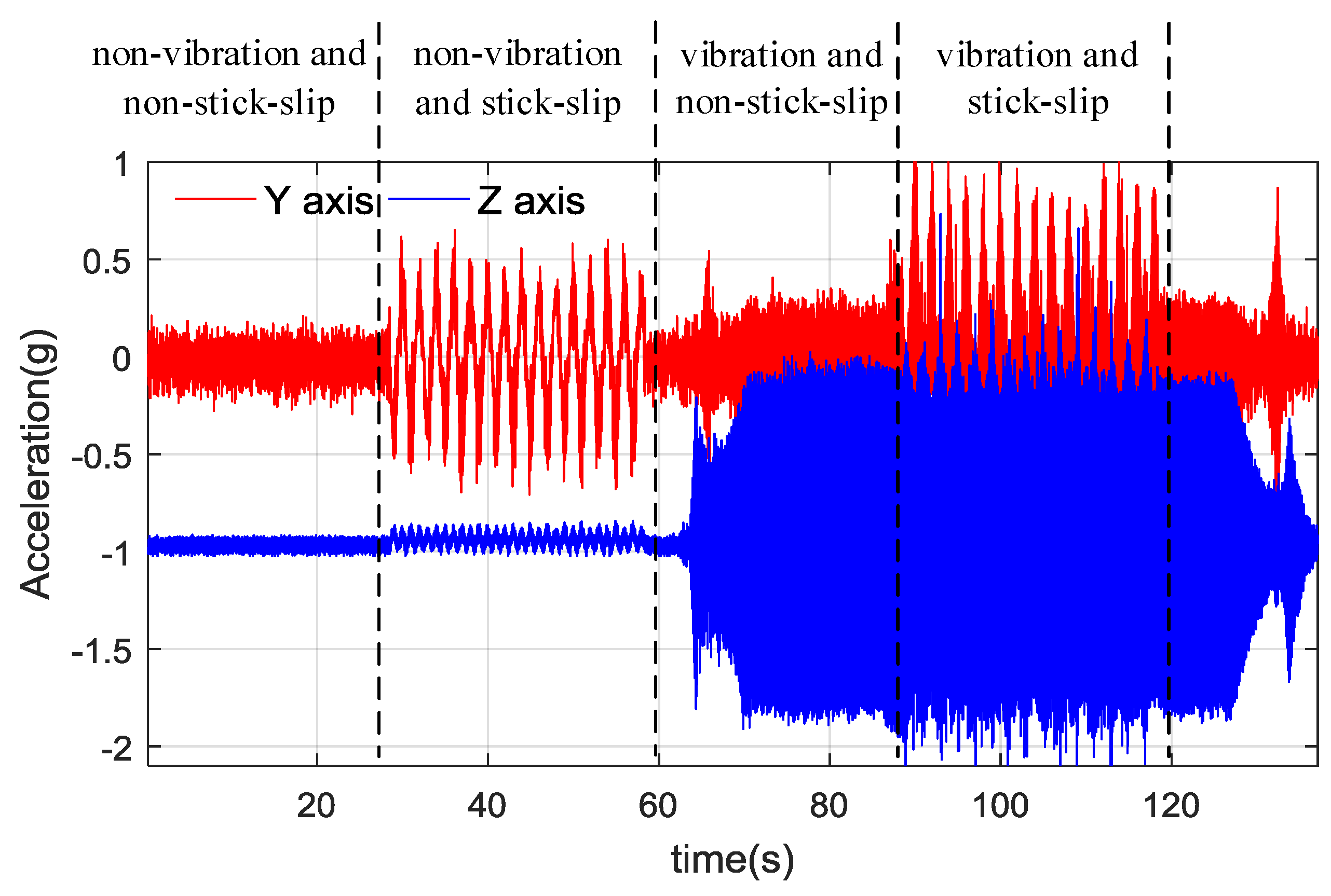
Figure 12.
Parameter tuning results. (a) RMSE value with different m and n. (b) RMSE distribution histogram.
Figure 12.
Parameter tuning results. (a) RMSE value with different m and n. (b) RMSE distribution histogram.

Figure 13.
Toolface estimation results and CF natural frequency in stick-slip test.

Figure 14.
The Y-axis and Z-axis acceleration measurements.
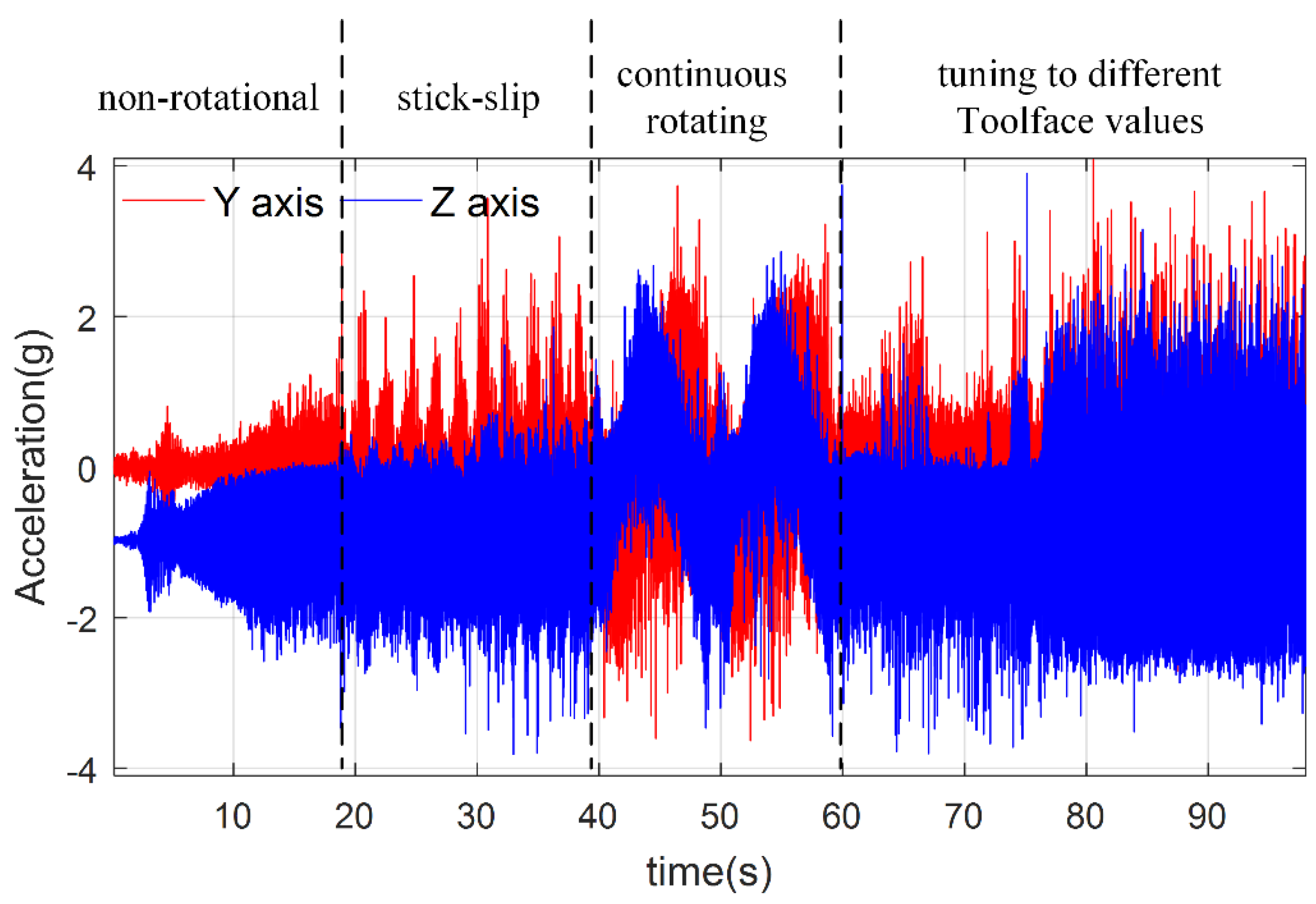
Figure 15.
Toolface estimation results and CF natural frequency in multi processes test.

Table 1.
Characteristics of Sensors.
| Parameters | Accelerometer | Gyro |
|---|---|---|
| Range | ±8 g | ±1200°/s |
| Sensitivity | 1024 counts/g | 0.83 mV/°/s |
| Bandwidth | 400 Hz | 40 Hz |
Table 2.
RMSE of Different Toolface Estimations in Stick-slip Test.
| Sources | Dual-Accelerometer | Gyro | Proposed CF |
|---|---|---|---|
| RMSE (°) | 18.022 | 11.6306 | 1.0069 |
Table 3.
RMSE of Different Toolface Estimations in Multi Processes Test.
| Sources | Dual-Accelerometer | Gyro | Proposed CF |
|---|---|---|---|
| RMSE (°) | 61.032 | 5.872 | 3.017 |
© 2018 by the authors. Licensee MDPI, Basel, Switzerland. This article is an open access article distributed under the terms and conditions of the Creative Commons Attribution (CC BY) license (http://creativecommons.org/licenses/by/4.0/).
Share and Cite
MDPI and ACS Style
Wang, W.; Geng, Y.; Wang, K.; Si, J.; Fiaux, J.D.O. Dynamic Toolface Estimation for Rotary Steerable Drilling System. Sensors 2018, 18, 2944. https://doi.org/10.3390/s18092944
AMA Style
Wang W, Geng Y, Wang K, Si J, Fiaux JDO. Dynamic Toolface Estimation for Rotary Steerable Drilling System. Sensors. 2018; 18(9):2944. https://doi.org/10.3390/s18092944
Chicago/Turabian StyleWang, Weiliang, Yanfeng Geng, Kai Wang, Jieru Si, and Joice De Oliveira Fiaux. 2018. "Dynamic Toolface Estimation for Rotary Steerable Drilling System" Sensors 18, no. 9: 2944. https://doi.org/10.3390/s18092944
Note that from the first issue of 2016, this journal uses article numbers instead of page numbers. See further details here.