Parameter Estimation of Lunar Regolith from Lunar Penetrating Radar Data
by
 ,
,
Ling Zhang
1,2, 
Zhaofa Zeng
1,2,*,
Jing Li
1,2,
Ling Huang
3,
Zhijun Huo
1,2,
Kun Wang
1,2 and
Jianmin Zhang
1,2 1
College of Geo-exploration Science and Technology, Jilin University, Changchun 130026, China
2
Ministry of Land and Resources Key Laboratory of Applied Geophysics, Jilin University, Changchun 130026, China
3
Institute of Electrics, Chinese Academy of Sciences, Beijing 100190, China
*
Author to whom correspondence should be addressed.
Sensors 2018, 18(9), 2907; https://doi.org/10.3390/s18092907
Submission received: 31 July 2018
/
Revised: 25 August 2018
/
Accepted: 31 August 2018
/
Published: 1 September 2018
(This article belongs to the Special Issue Sensors, Systems and Algorithms for GPR Inspections)
Abstract
:Parameter estimation of the lunar regolith not only provides important information about the composition but is also critical to quantifying potential resources for lunar exploration and engineering for human outposts. The Lunar Penetrating Radar (LPR) onboard China’s Chang’E-3 (CE-3) provides a unique opportunity for mapping the near-surface stratigraphic structure and estimating the parameters of the regolith. In this paper, the electrical parameters and the iron-titanium content of regolith are estimated based on the two sets of LPR data. Firstly, it is theoretically verified that the relative dielectric constant can be estimated according to the difference of the reflected time of two receivers from a same target. Secondly, in order to verify the method, a parameter estimation flow is designed. Subsequently, a simple model and a complex model of regolith are carried out for the method verification. Finally, on the basis of the two sets of LPR data, the electrical parameters and the iron-titanium content of regolith are estimated. The relative dielectric constant of regolith at CE-3 landing site is 3.0537 and the content of TiO2 and FeO is 14.0127%. This helps us predict the reserves of resources at the CE-3 landing site and even in the entire Mare Imbrium.
1. Introduction
As said in Reference [1], the surface of the Moon has collided with small and large asteroidal and cometary materials for 25 billion years. As time passes, these collisions comminute the surface materials and ‘gardened’ a fine-grained layer termed “regolith.”The thickness of the regolith is between 2 and 20 m, beneath the younger maria and below the oldest surface of the lunar highland separately. Parameter estimation of the lunar regolith not only provides important information about its composition but is also critical for quantifying potential resources for lunar exploration and engineering for human outposts.
The regolith parameter could be determined by the experiments of return samples from the lunar surface. The Luna and Apollo programs have collected lunar regolith and rock samples on the lunar surface and were returned to Earth. Laboratory experiments of these samples have been conducted to reveal the nature of lunar regolith. Basu et al. [2] estimated the average chemical composition and mineral composition of lunar regolith in each sampling area, according to the lunar samples of the Apollo and Luna projects; Carrier et al. [3] and Gromov et al. [4] calculated the relationship between the mechanical properties of regolith and its density; Sen et al. [5] and Olhoeft et al. [6] measured the complex permittivity of lunar samples and fitted their relationship to density.
Some early ground-based observations and remote sensing methods also studied the nature of lunar regolith. Krotikov et al. [7] used a ground-based radio telescope to analyze the mechanical properties of lunar regolith; Tyler [8] analyzed the properties of regolith based on the Explorer electromagnetic echo; Alan et al. [9] and Pollack et al. [10] analyzed the relationship between the dielectric constant and density of large regions, such as highlands and basins, by using radar echo; Pommero et al. [11] analyzed the mineral composition, especially the iron and titanium content, with the Lunar Radar Sounder (LRS) data of the SELENE mission. These long-range detection methods can detect large areas but their accuracies are low.
The third method of parameter estimation is the in-situ detection. Lunokhod rovers and Apollo astronauts have conducted a great deal of research on the physical properties of lunar regolith but they are aimed at the mechanical properties of regolith, while the electrical properties have not been studied. On 14 December 2013, Chang’E-3 landed at 340.4875° E, 44.1189° N on the Mare Imbrium. LPR on the rover detected near-surface geological formations and the parameters of lunar regolith in the inspection area [12].
The dual-frequency Lunar Penetrating Radar aboard the Yutu Rover provides three sets of data: a set of data from the low-frequency channel (CH-1, 60MHz) to map the subsurface structure to a depth of several hundreds of meters and two sets of data (CH-2A and CH-2B) with different offsets from the high-frequency channel (CH-2, 500MHz), to detect the regolith [13].
LPR data processing and initial results are first presented by NAOC (National Astronomical Observatories, Chinese Academy of Sciences) [14]. Initial analysis of the LPR observations, especially that from CH-1, indicate that there are more than nine subsurface layers from the surface to a depth of ~360m [12]. The onboard Lunar Penetrating Radar conducted a 114m long profile, measuring a thickness of the lunar regolith layer of ∼5 m and detecting three underlying basalt units at depths of 195, 215 and 345 m. The radar measurements suggest an underestimation of the global lunar regolith thickness by other methods and reveal a vast volume from the last volcanic eruption [15]. Fa et al. [16] and Lai et al. [17] estimated the near surface structure by processing the raw CH-2 data.
Ground Penetrating Radar (GPR) is a non-destructive testing technology which is widely used in a variety of applications, such as, geophysical detection, planetary sensing, civil engineering and environmental monitoring. The main purpose is locating and imaging the hidden targets by electromagnetic detection [18]. LPR is just the application of GPR in lunar exploration. Parameter estimation of radar data is an important direction of GPR technology. A common midpoint method is the most common method of estimating the dielectric constant, which is used arange of transmitter-to-receiver offsets, assuming that the reflector is present in the ground and aligned with the midpoint between the antennas. A set of simultaneous equations involving propagation and times baseline lengths allows one to solve the dielectric constant [19]. SIMO (Single Input Multiple Output) and MIMO (Multiple Input Multiple Output) are other typical applications which are the same as this method [20,21]. The second technique involves the presence of buried point scatterers that will produce a hyperbolic radar return (the propagation time in a B-scan relative to the position of radar). The dielectric constant can be obtained by characterizing the shape of this hyperbola [22] or found by using inverse scattering algorithms with a range of prospective permittivity values [23]. The third set of techniques is trying to use a complex and often full-wave method to simulate the radar on top of the dielectric ground and coupling these with iterative optimization techniques to find the dielectric constant that matches the simulation to measurements [24,25]. In the fourth method, a more direct method can be used to design probes that penetrate the soil or extract soil samples and measure using standard laboratory permittivity [26,27,28,29,30]. The fifth approach turns to crosstalk between the transmitter and the receiver of the ground-coupled bistatic radar, with small to negligible antenna spacing. In References [31,32], the dielectric constant estimation of crosstalk frequency variation due to the presence of ground is briefly introduced. In the sixth approach, the authors estimate parameters by using the various information of the traces, such as the travel time [33], phase [34], amplitude [35], frequency spectrum [36], reflection coefficient [37], direct wave [38] and so on.
Some pre-research used LPR data to estimate the parameters of lunar regolith. Dong et al. [39] calculated the parameters of the regolith by relative reflection amplitudes; Feng et al. [40] estimate the radar velocity and the parameters of the regolith by hyperbolic matching in the CH-2B radar-gram.
In this paper, two sets of data (CH-2A and CH-2B) are used to estimate the dielectric constant of lunar regolith and the iron-titanium content. Firstly, we introduce the principle and the formula derivation of the method. Secondly, we design a flow for model verification and parameter estimation. Thirdly, a complex regolith model is carried out for the verification of this method in lunar regolith estimation. Finally, the dielectric constant and the content of TiO2 and FeO in lunar regolith are estimated from LPR data.
2. Methodology
In this paper, the parameter estimation method uses two sets of radar data with different offsets. According to the difference of the arrival time of the two sets of data from the same target, we can estimate the dielectric parameters.
This section will divide into two cases. The first case: There is no space between the radar and the ground. In the second case, there is space between the radar and the ground.
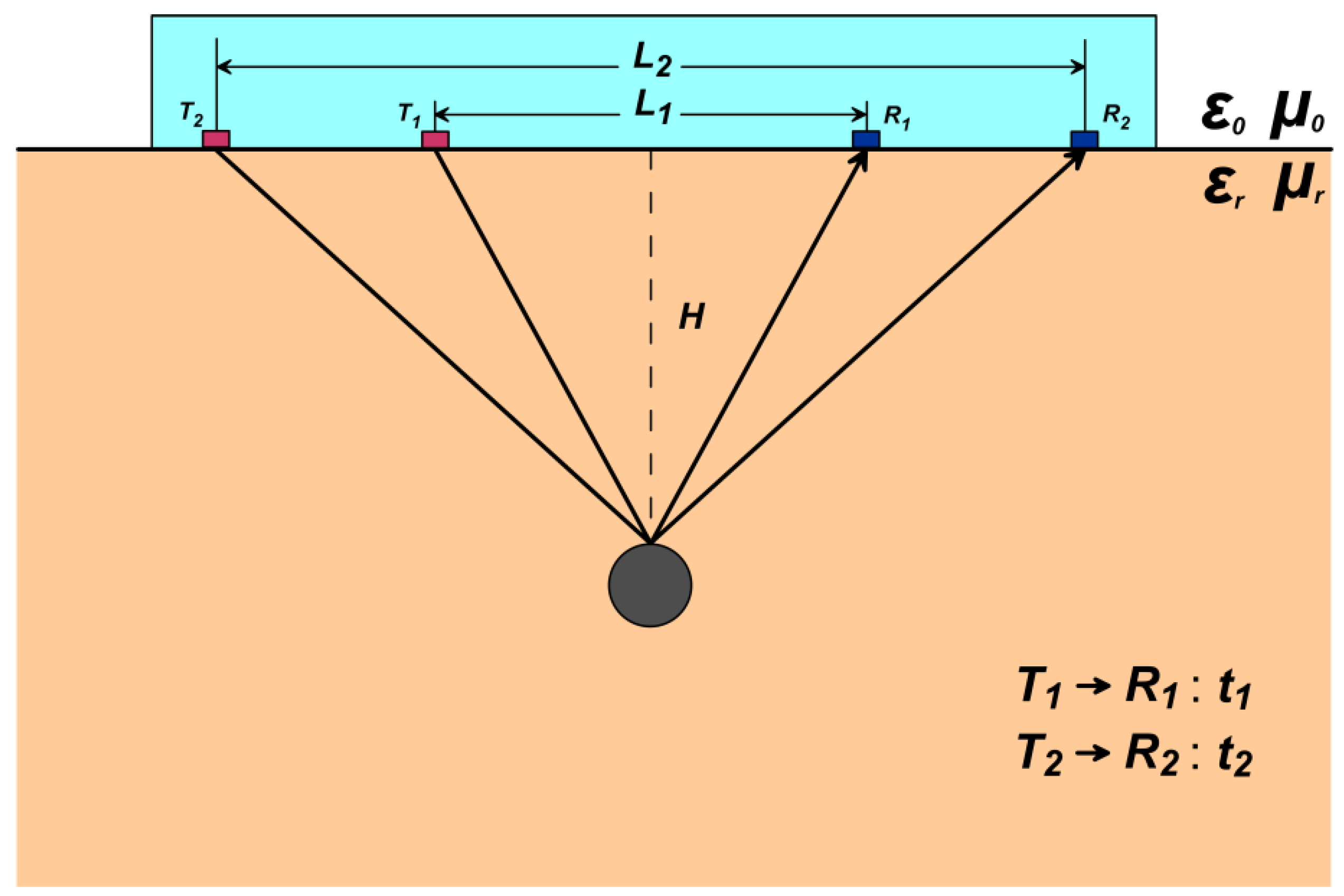
Figure 1 illustrates the geometric propagation paths of electromagnetic waves when the two sets of radar transmitters () and receivers () with different offsets () are close to the ground. The dielectric constant of the medium is estimated by the different arrival time (&) of the reflected waves from a same anomalous body.
According to the geometric relationship of Figure 1, it can be known that:
where is the time of the electromagnetic wave from to when the offset is , is the time of the electromagnetic wave from to when the offset is and is the velocity of the electromagnetic wave in the medium.
The relationship between the electromagnetic wave propagation velocity and the electrical parameters (dielectric constant and magnetic permeability) is known:
where is the dielectric constant and is the magnetic permeability, is the velocity of electromagnetic waves in a vacuum.
Obtained from Equations (1) and (3) and Equations (2) and (3):
and from Equations (4) and (5):
for two sets of data with different offsets, when:
- (1)
- the transmitter and receiver are close to the ground;
- (2)
- the offsets () are known;
- (3)
- the reflected time () is known; and
- (4)
- the medium is a non-magnetic medium (),
According to Equations (6) and (7), the position of the abnormal body and the dielectric constant of the medium can be estimated.
In the actual situation, the radar transmitter and receiver are difficult to get close to the ground. Generally, there is a certain height from the ground to the radar.
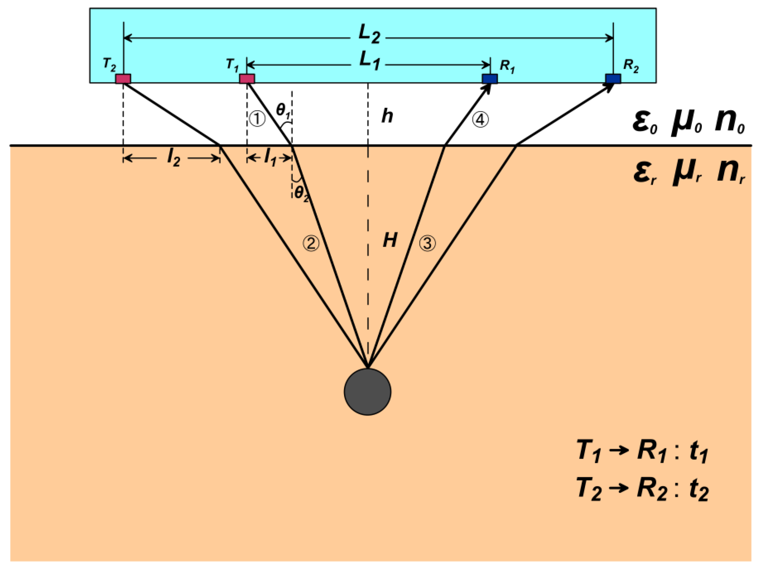
Figure 2 illustrates the geometric propagation paths of electromagnetic waves when the two sets of radar transmitters () and receivers () with different offsets () are at a height () over the ground.
Take the path from to as an example:
Snell’s Law:
where is the incident angle of the electromagnetic wave, is the angle of refraction, and are the refractive index of the vacuum and the medium, respectively.
The velocity of electromagnetic waves in the medium:
is the refractive index of the medium, and are the relative permittivity and the relative permeability of the medium, is the velocity of electromagnetic waves in vacuum.
Bringing Equations (9)–(12) into Equation (8) and sort out:
According to the electromagnetic wave path and the velocity, the time from to :
In the same way, we can get the relationship from to :
In the four Equations (13)–(16), there are 11 parameters (). When:
- (1)
- the offsets () are known;
- (2)
- the height () of the radar from the ground is known;
- (3)
- the reflected time () is known; and
- (4)
- the medium is a non-magnetic medium ().
The four remaining unknown parameters can be obtained according to the four Equations (13)–(16). Thereby, we can estimate the position of the abnormal body and the dielectric constant of the medium.
3. Permittivity Estimation Procedure
According to the following steps, the same model (Figure 3a and Figure 5a) is used to describe the above two cases.
Step 1: Simulation. Setting different parameters perform simulations of the model and we can obtain two sets of radar profiles with different offsets.
Step 2: Obtain and . Read the reflection arrival time of the two sets of data from the same target. Specific operations of step 2:
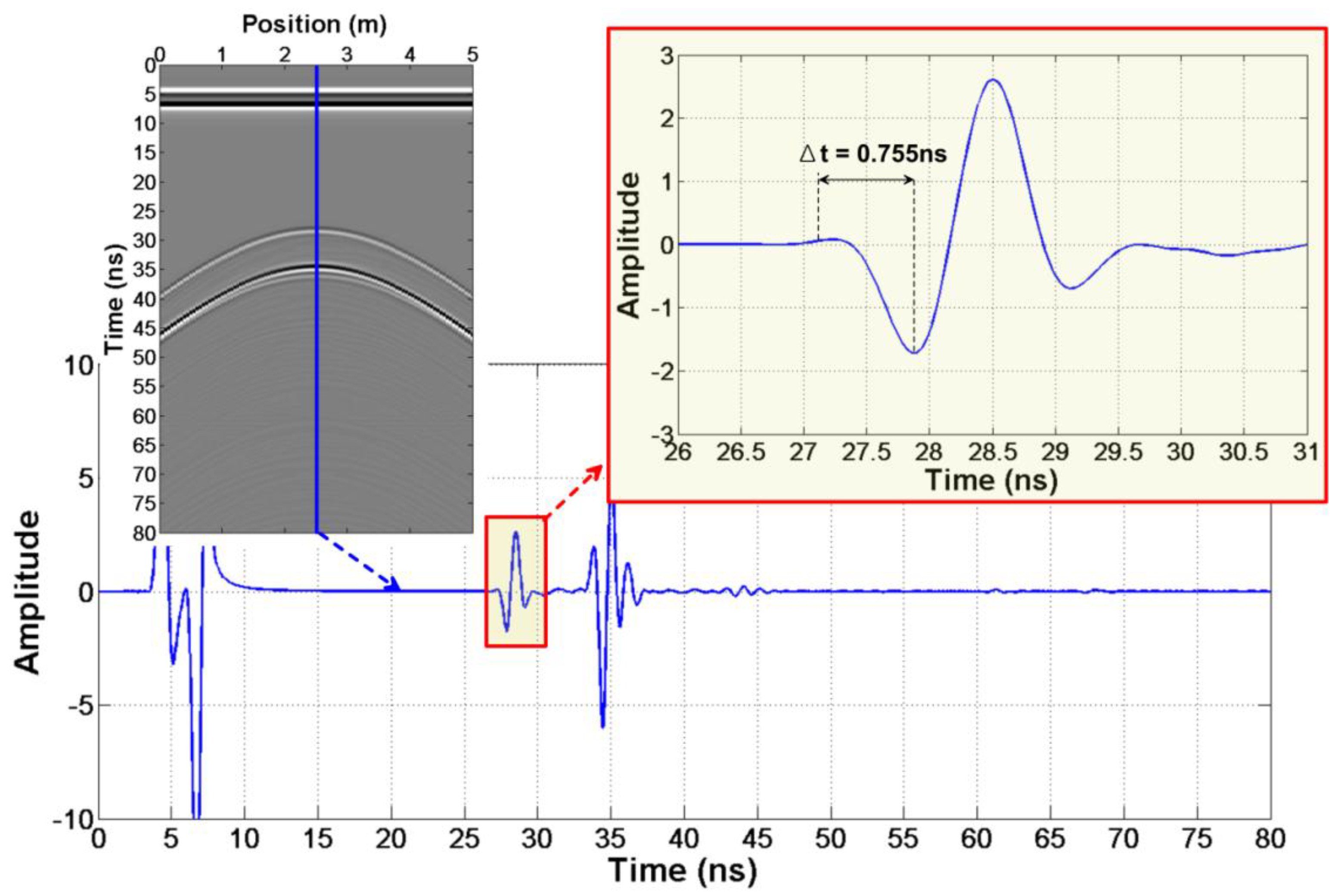
Step 2.1. Firstly, read the first significant extreme point of the reflected wavelet and get , .
Step 2.2. Then, extract a reflected wavelet from the radar profile and read the time from the jump point to the first significant extreme point in the wavelet.
Step 2.3. Finally, the true reflected wave arrival time of the data with different offsets is obtained , .
Step 3: Parameter estimation. The dielectric constant is obtained according to the Equations (6) and (7) or Equations (13)–(16) for different situations.
The two cases are specifically described below.
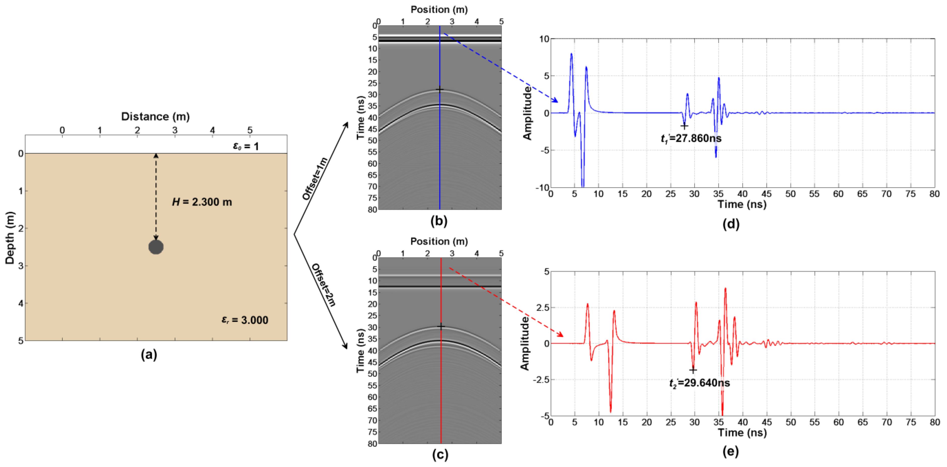
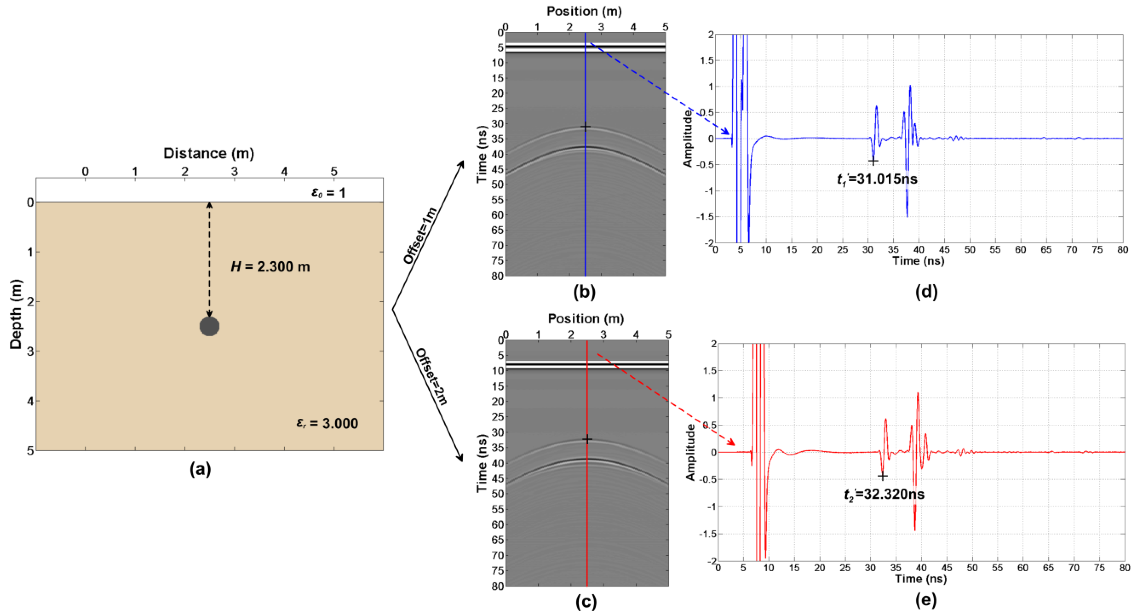
Firstly, the simulation of the forward modeling (Figure 3a) have been done. FDTD (Finite-Difference Time-Domain) is applied for the simulation of the simple model. The FDTD main code was written by Irving and Knight [41] but we modified some parts of the code (the import of the model, the export of the wavefield snapshot and so on). Some key simulation parameters are presented in Table 1 and we obtain two sets of radar profiles with different offsets (Figure 3b,c).
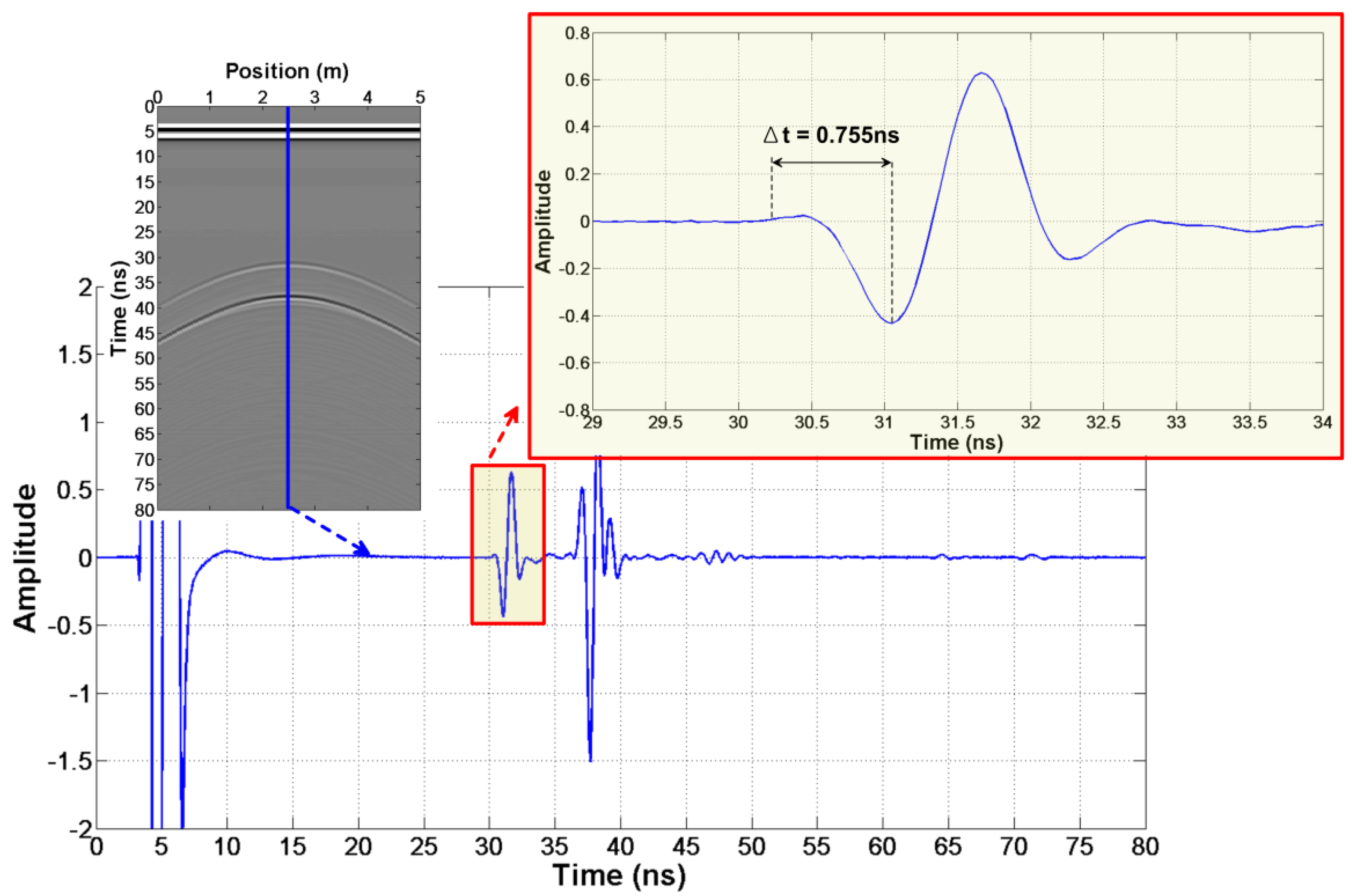
According to step 2, we firstly read out and in Figure 3d,e. Then, we get from the wavelet waveform (Figure 4). Finally, the true arrival time and are obtained.
Consistent with the second case, the model (Figure 5a) is simulated firstly and the parameters are shown in Table 1. Two sets of radar profiles with different offsets are obtained (Figure 5b,c). What is different from the first case is that the radar transmitter and receiver is of 0.5 m above the ground.
According to step 2, we firstly read out and in Figure 5d,e. Then, we get from the wavelet waveform (Figure 6). Finally, the true arrival times and are obtained.
Finally, following the third step, as we have already known some parameters, the quaternary equations shown below are obtained by using the Equations (13)–(16).
The solution, , , which is solved by least squares, is consistent with the model. Thus, the method is feasible.
4. Model Experiment
In order to verify the feasibility of the method on the moon, this section conducts model tests. Two models are established: the first one is a simple model with different anomalous bodies and the second one is a complex regolith model. Verification shows that this method is feasible to estimate the electrical parameters of the regolith.
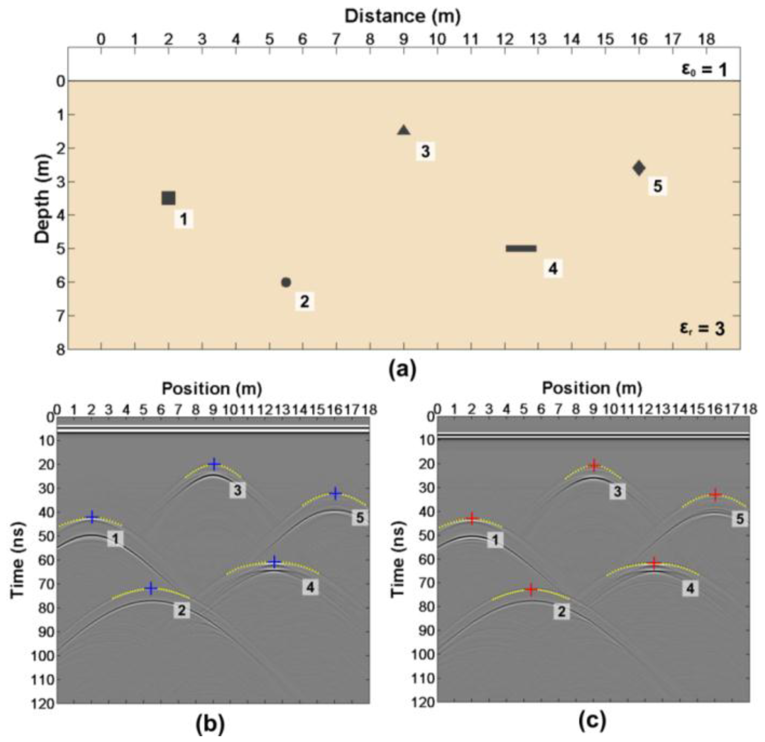
The simple model is built as shown in Figure 7a, in which there are five anomalous bodies with different shapes. The relative dielectric constant of the anomalous body is 6. Figure 7b,c shows the forward results with different offsets of 1 m and 2 m, respectively. The forward parameters are shown in Table 2.
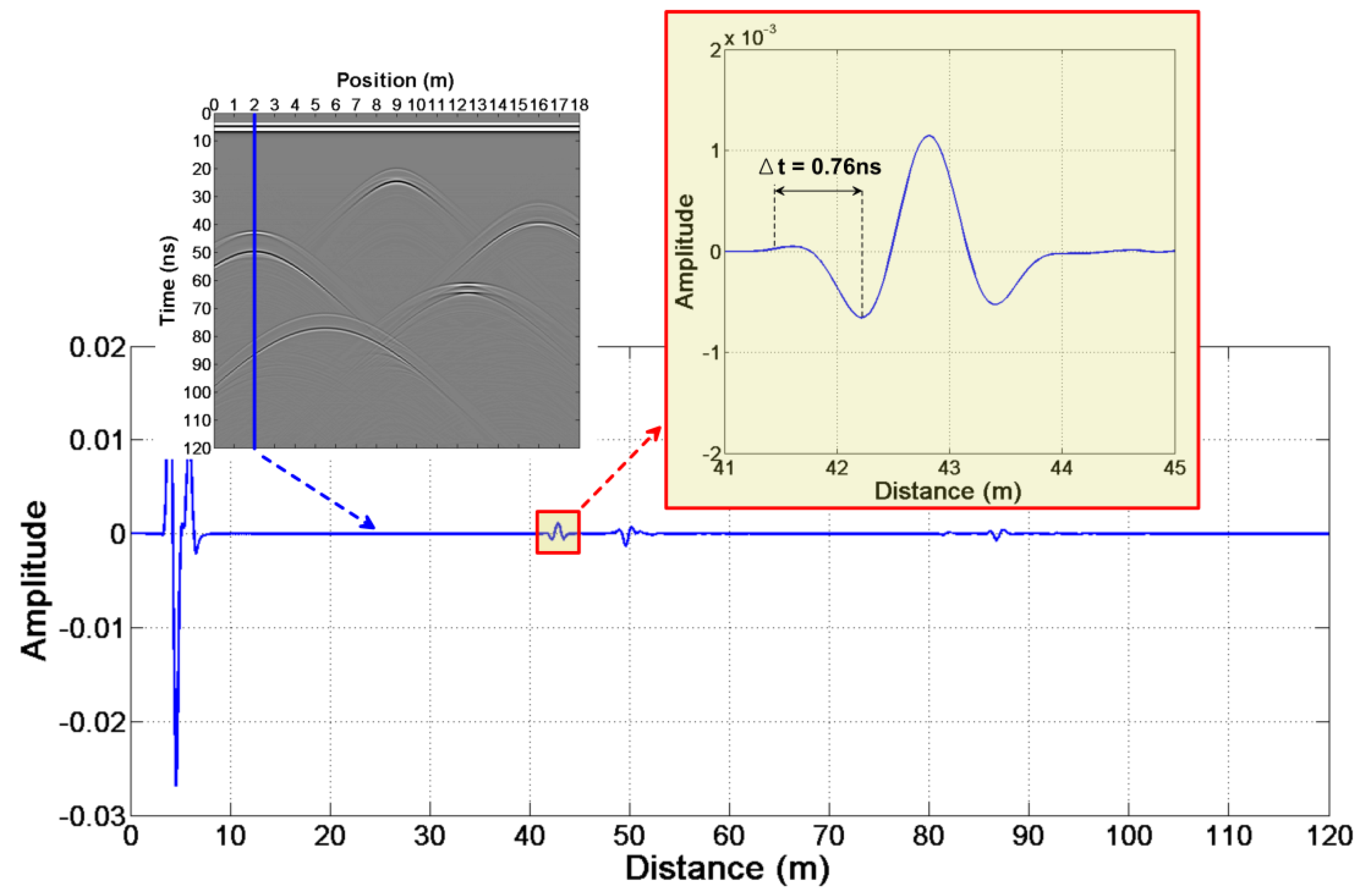
According to the above steps of this method, we can read the arrival time at each position (Table 3). We know from Figure 8. The height of the anomalous bodies and the relative dielectric constant (Table 3) can be estimated by the Equations (13)–(16).
We consider several approaches to obtain the final estimated dielectric constant:
- (1)
- The final result is calculated by the mean of the recovered permittivity values:where is the final estimated dielectric constant, is the number of the recovered permittivity values and is the ith recovered permittivity value.
- (2)
- A weight based on the amplitude of the measured echoes is set:where is the final estimated dielectric constant, is the number of the recovered permittivity values and is the ith recovered permittivity value. is ith amplitude.
- (3)
- A weight based on the reciprocal of the estimated height of each anomalous body is set:where is the final estimated dielectric constant, is the number of the recovered permittivity values and is the ith recovered permittivity value. is ith height.
After a comprehensive consideration, we set a weight based on the reciprocal of the estimated height of each anomalous body as the final result. Since if the standard deviation of the recovered permittivity values is quite large, calculating the mean of the recovered permittivity values is too simple and is not a reliable methodology. However, if the radar data has a low signal-to-noise ratio and a high energy attenuation, it is too difficult to obtain the real amplitude of the reflection waves. If the reference target is particularly deep, the estimation could become sensibly inaccurate, so setting a weight based on the reciprocal of the estimated height of each anomalous body as the final result could be an easy and reliable method.
The estimated dielectric constant is:
which is consistent with the model.
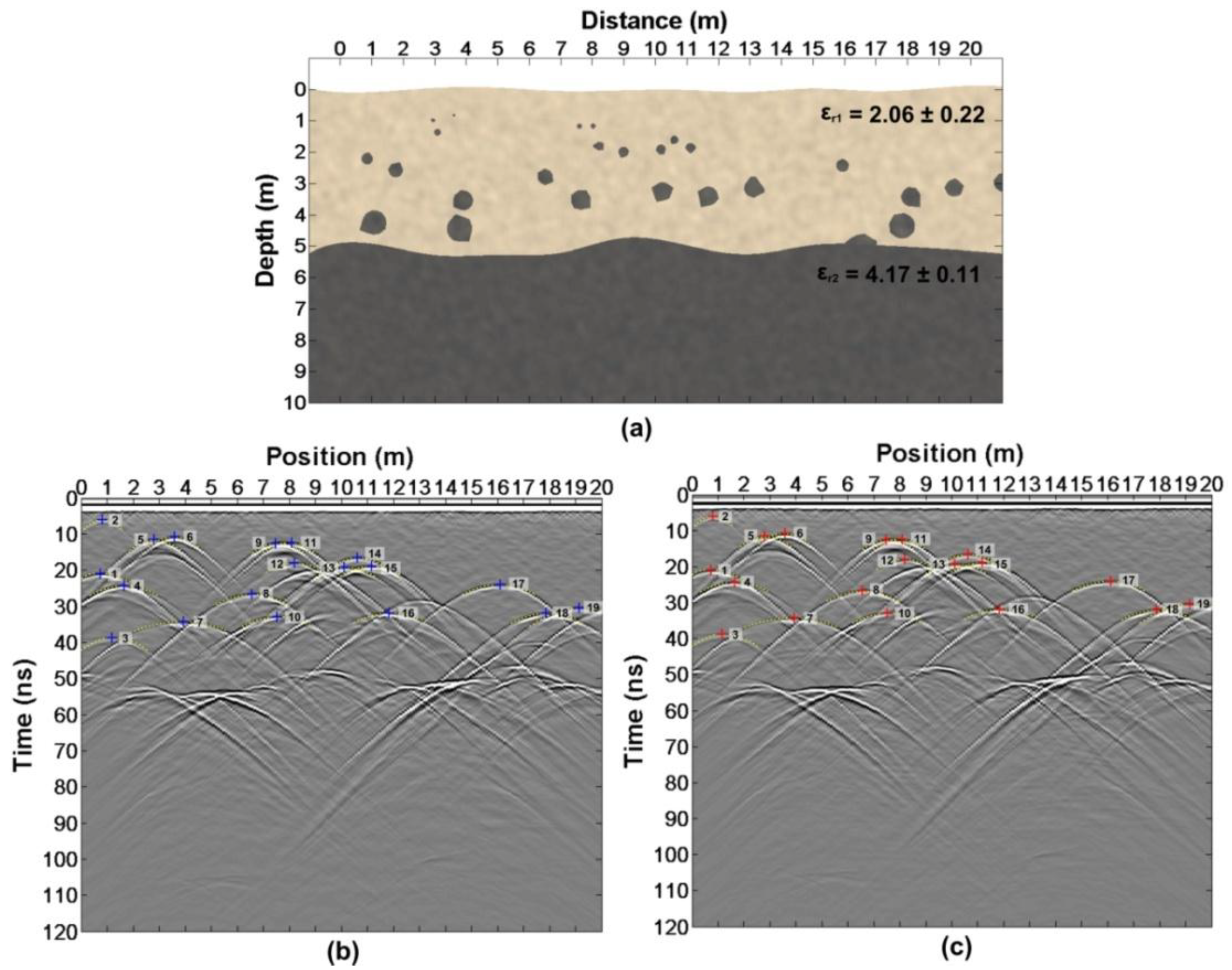
In order to verify whether this method is suitable for LPR data, we build a complex model (Figure 9a). This model considers many factors: random medium, undulating interface and anomalous body. The modeling method is referenced in References [42,43,44]. According to the actual acquisition parameters of LPR [13], the simulated parameters are shown in Table 2. Two sets of forward results with different offsets are obtained in Figure 9b,c. According to the above method, reading from the two sets of radar data, and are shown in Table 4. is from Figure 10. The height and the relative dielectric constant (Table 4) are estimated according to the Equations (13)–(16).
It can also be found that for this kind of complex data the variance of the result is relatively large (the standard deviation is quite large) due to the non-uniformity of the medium, so, as mentioned above, we set a weight based on the reciprocal of the estimated height of each anomalous body as the final result. The estimated final dielectric constant is:
This is consistent with the forward complex model ().
5. Result
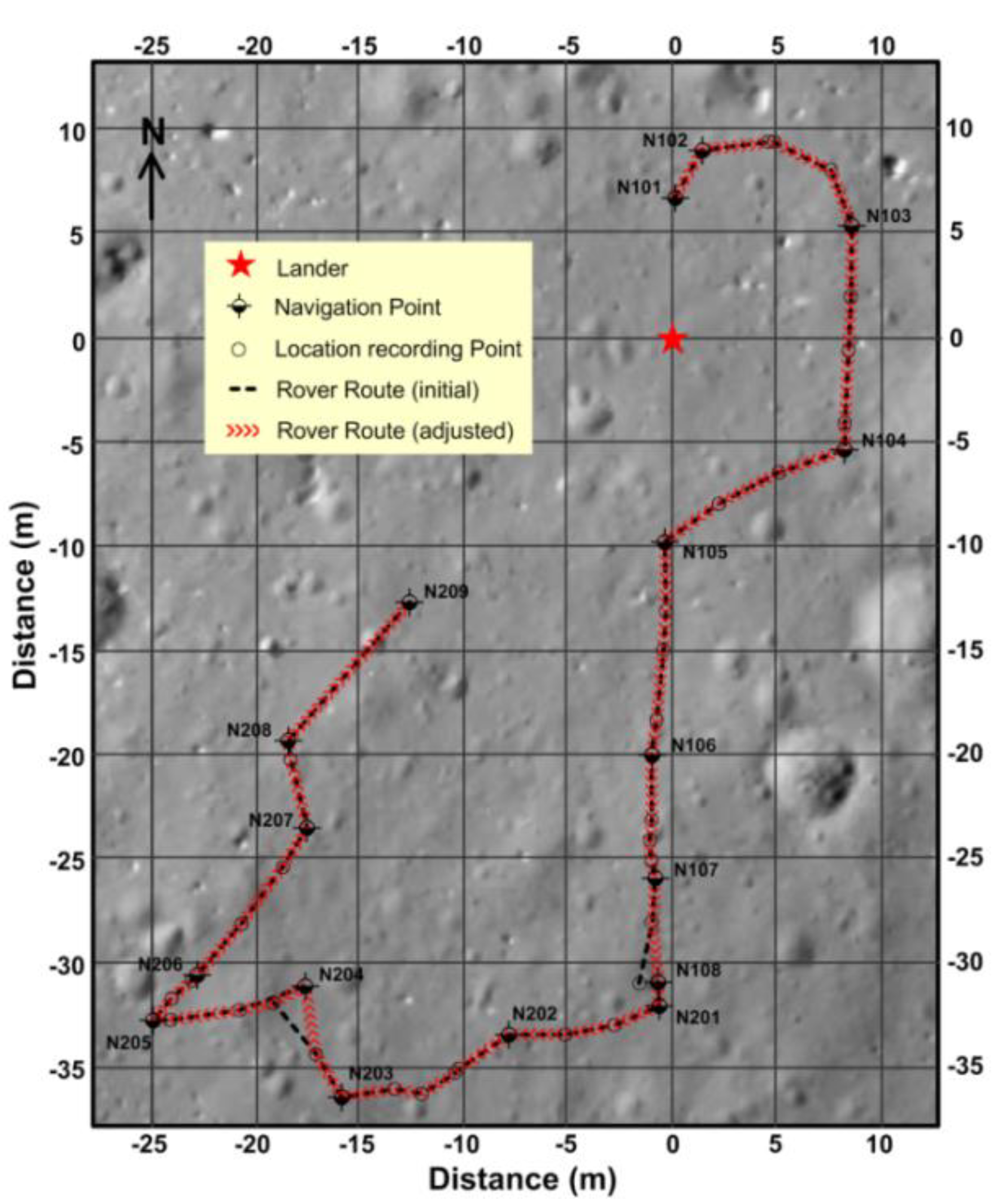
The Yutu rover released by CE-3 was the first soft landing on the Moon since the Soviet Union’s Luna 24 mission in 1976. To be specific, the Yutu rover explored the surface and subsurface of the landing site in the northern part of Mare Imbrium using its four main instruments: The Panoramic Camera, Lunar Penetrating Radar (LPR), Visible–Near Infrared Spectrometer (VNIS) and Active Particle-Induced X-ray Spectrometer (APXS). Its track extends to 114.8 m (Figure 11) near a young crater. In this part, the data processing results of the LPR are reported.
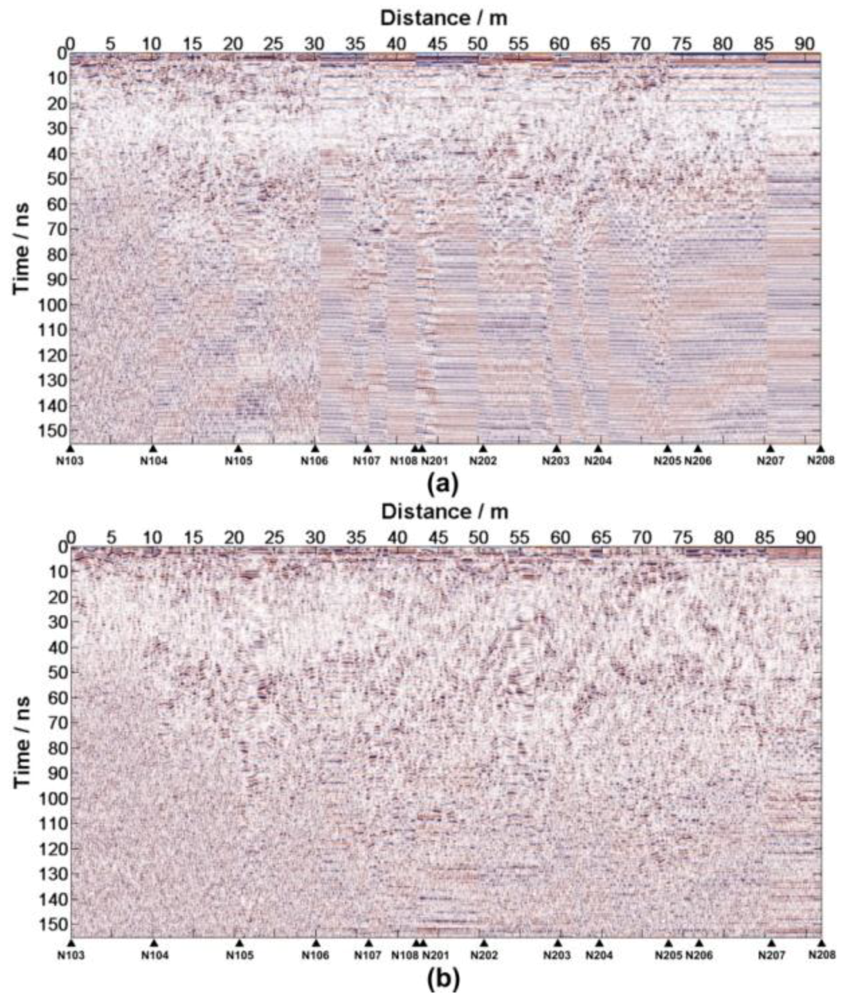
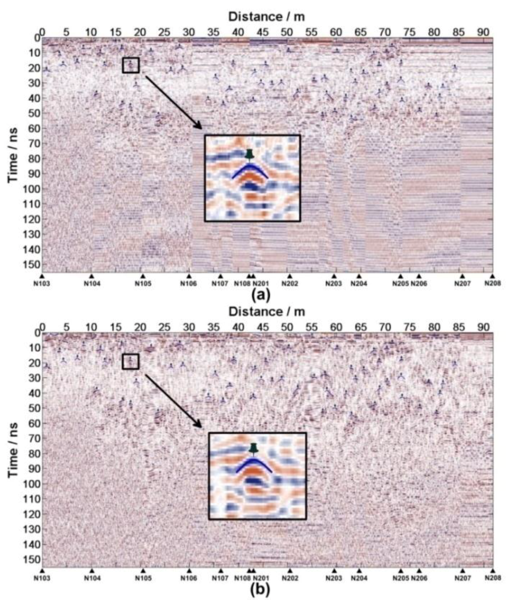
Aiming at the near-surface stratigraphic structure of the regolith, the CH-2 data is selected. TheCH-2 has two receiver antennas (CH-2A and CH-2B).The LPR data processing pipeline is designed according to the acquisition parameters, the actual situation and the data quality (Table A1 in Appendix A). Two radar images with high resolution (Figure 12) are accessible after data editing and processing. The IDs for the data from Lunar Penetrating Radar are listed in Table A2 in the Supporting Materials.
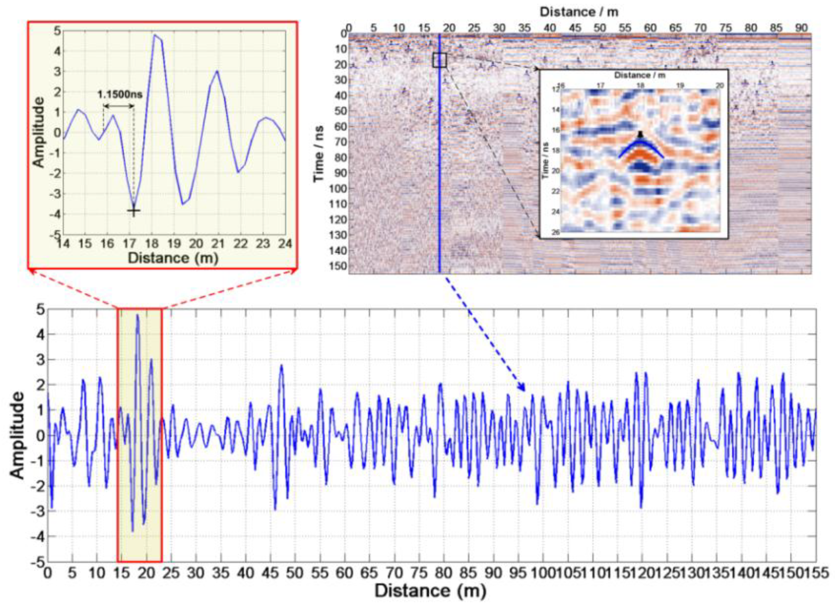
At first, the reflected waves caused by the same basalt block should be found in CH-2A and CH-2B data (Figure 13). Reading the and of each position follows according to Figure 14, . Equations (13)–(16) estimate the height and the relative dielectric constant of each anomaly body, which are shown in Table A3.
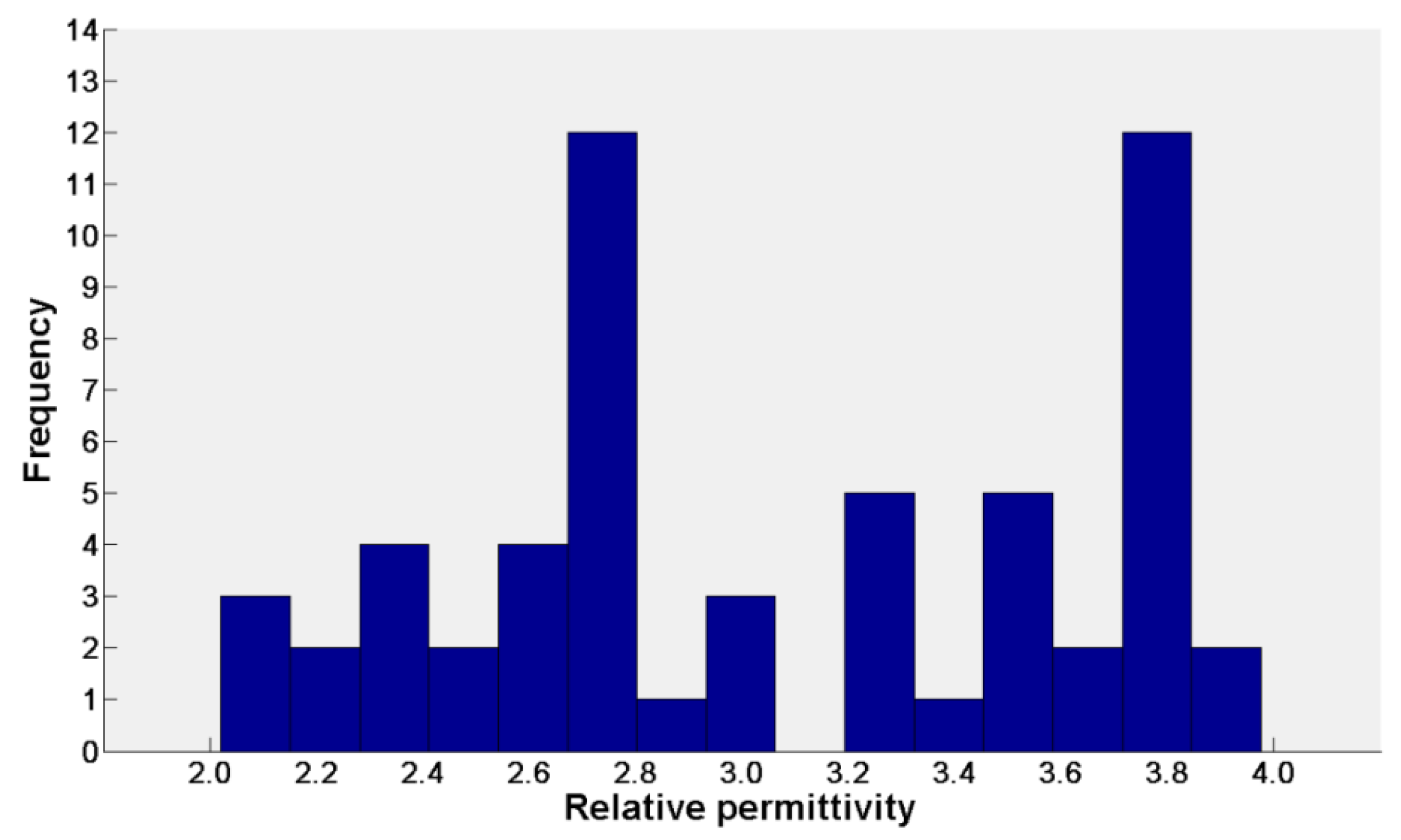
In order to support the conclusion in this paper, deep statistical analysis of the results should be conducted. A histogram of the recovered permittivity is shown in Figure 15.
If we only focus on the analysis of the recovered permittivity data ( in Table A3), the mean value of the estimated dielectric constant is , the standard deviation is . However, as with the previous analysis, we believe that if the weight based on the reciprocal of the estimated height of each anomalous body is applied, the estimated dielectric constant is much more accurate:
and the standard deviation:
We believe that the recovered permittivity obeys the normal distribution, the estimated final dielectric constant is (confidence level at 95%).
According to the above result, a reasonable dielectric constant result has been given but it is found from Figure 15 that the recovered dielectric constant distribution is not a standard normal distribution and the standard deviation is also relatively large. We consider it is due to the heterogeneity of the regolith medium. The recovered dielectric constant is not only related to the location but also related to the depth. An analysis between permittivity and the depth (or location) of the target should be performed to improve data post-processing.
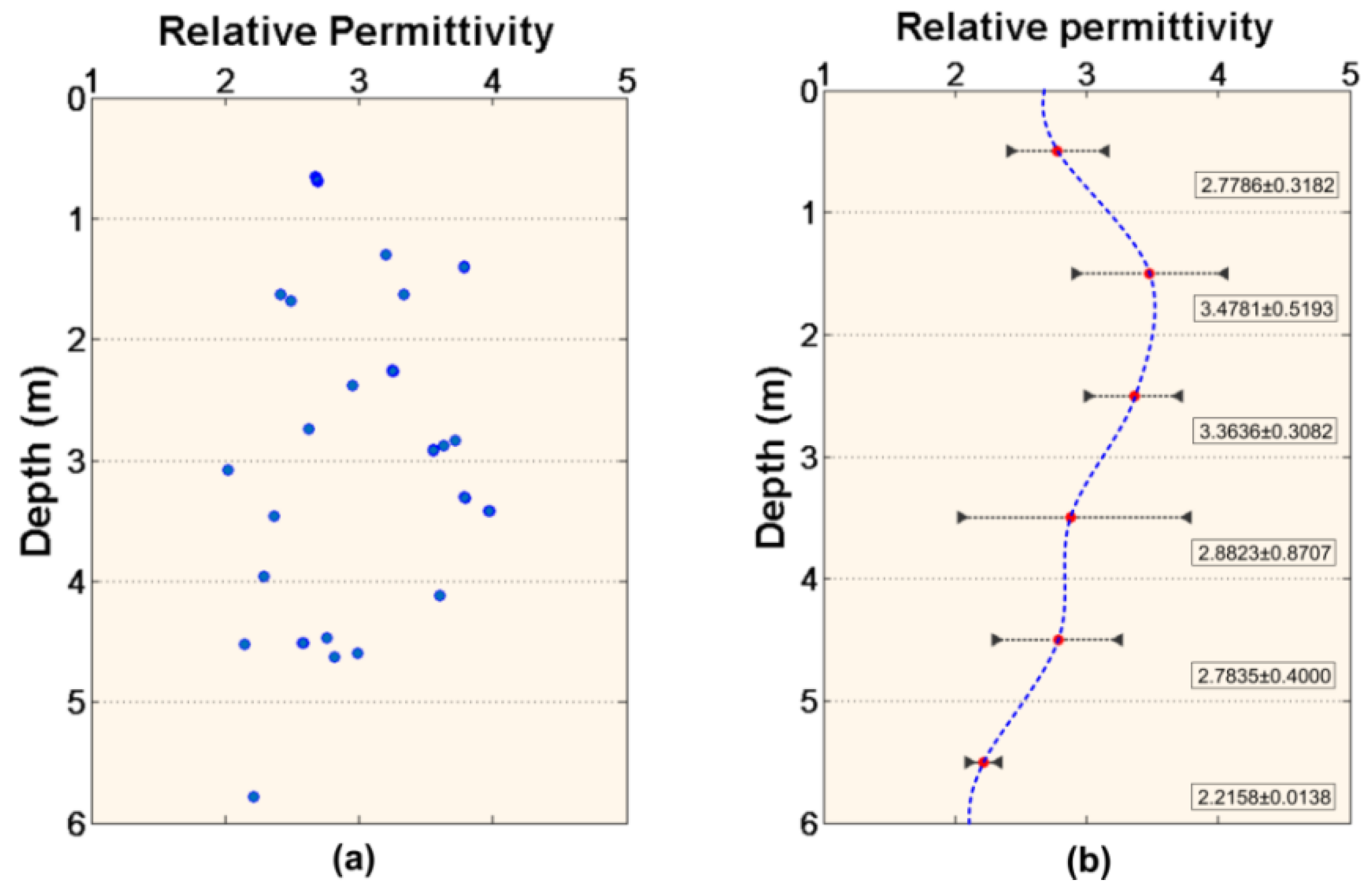
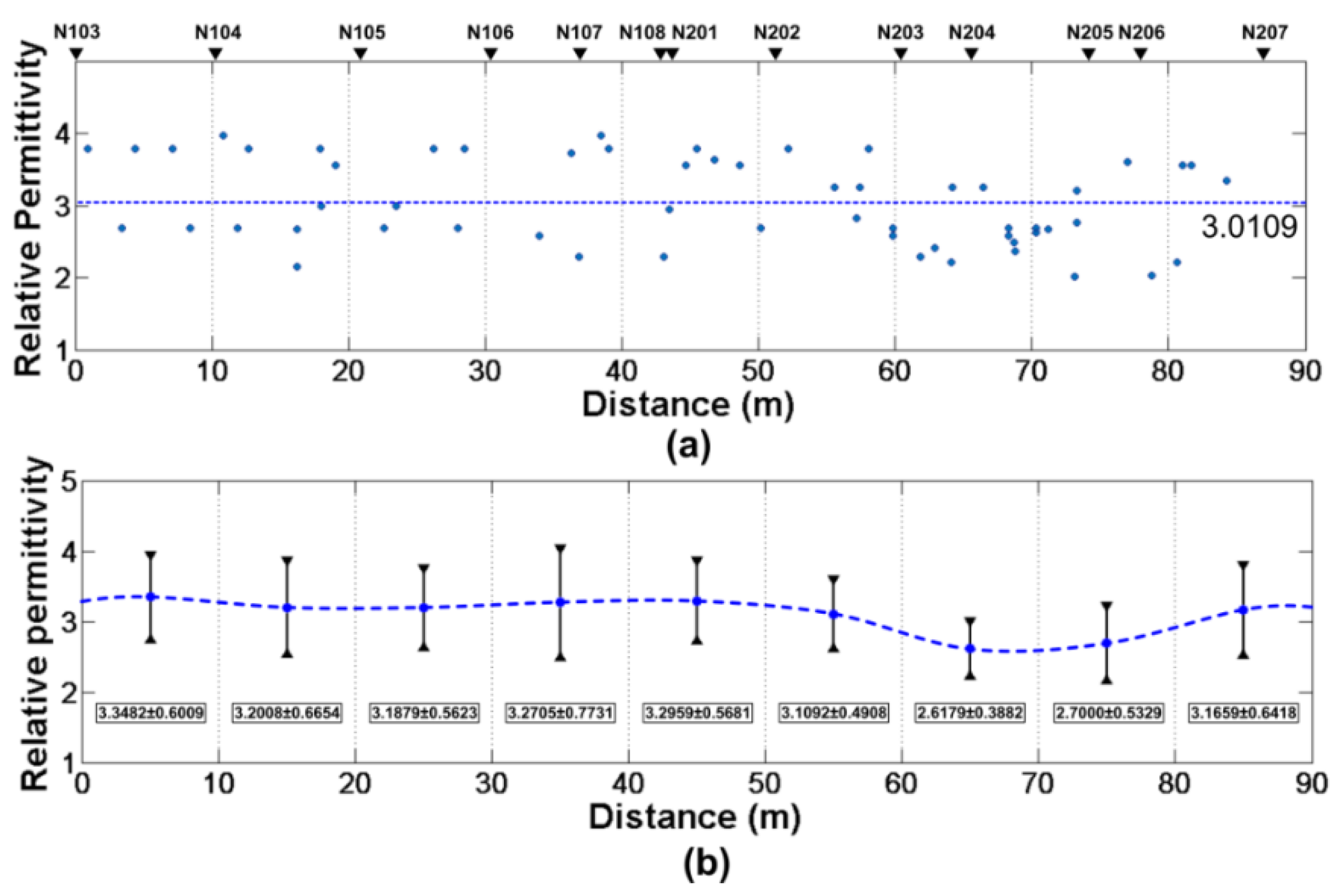
Figure 16a is scatterplot of permittivity and depth and at each meter, we calculate the mean values and the standard deviations (Figure 16b). The figure shows us a relationship between permittivity and depth. There is a maximum value at ~2m, which is due to the stratigraphic structure at the CE-3 landing site. At the same way, the analysis between permittivity and the location of LPR has been performed in Figure 17. The permittivity does not change drastically with location.
The lab test results from lunar regolith samples on Apollo and Luna era show that the dielectric constant of lunar regolith is related to the density of lunar regolith [1]. The density is yielded by the dielectric constant as follows:
The loss tangent (tan δ) can be easily yielded by the density as follows:
and:
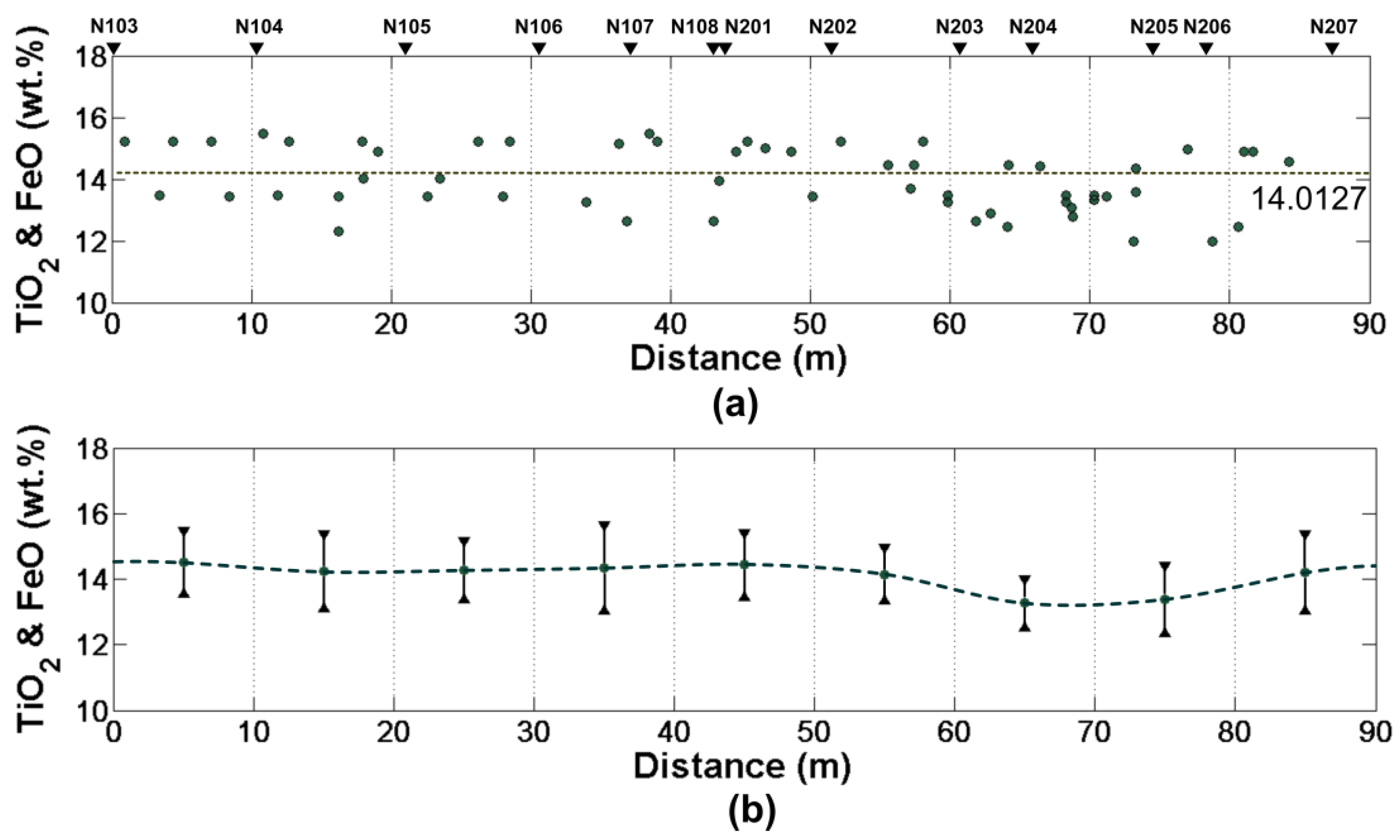
On the basis of the obtained relative dielectric constant, On the basis of the obtained relative dielectric constant, the content of TiO2 and FeO on CE-3 landing site were estimated (the results are shown in Figure 18).
6. Discussion
The method for permittivity estimation in this paper has the advantages compared with the method mentioned in the introduction:
- (1)
- It is easier to understand and operate. This method uses two sets of data with different offsets to estimate the permittivity. The main work is reading the arrival times of the same anomalous body. It is easier to operate than the methods in the introduction, since the various methods need to extract complex information, such as amplitude, spectrum, phase and so on.
- (2)
- The data quality requirements are lower, even if the radar data contains various types of noise, so as to affect the data waveform, amplitude and frequency, it will not affect the applicability of this method.
- (3)
- No prior information and other data are needed. This method does not require any a priori information, such as incident wave information and does not require other data, such as TDR (Time-Domain Reflectometry) data and so on.
- (4)
- It is more suitable for the LPR data collected by CE-3 mission. The original intention of this method is only for the parameter estimation of LPR data. The before methods depend on the low signal-to-noise ratio of the data and need to have all kinds of accurate information, while LPR data is collected on the moon, various types of noise affect the signal-to-noise ratio of the data and deep processing, including gain, filtering, background removal and so forth, has to be done which affected the nature of the data. The method in this paper only needs the information of the arrival time to perform parameter inversion.
However, it is undeniable that this method also has disadvantages compared to other methods. Two sets of data with different offsets are required. It is necessary to extract an accurate wavelet. Only the dielectric constant can be estimated and the conductivity is ignored. This method is only applied in the case of containing various types of scatterers.
Since this method is mainly aimed at the inversion of the lunar soil parameters, it is still a good predictor for the parameters of the lunar regolith.
There are also many factors which will affect the accuracy of the result when using this method for the parameter estimation:
- (1)
- Sampling rate. Horizontal and vertical sampling rate will determine the resolution of the radar profile, which will affect the accuracy.
- (2)
- Offset. The distances of transmitters and receivers will also affect the result. In general, the larger the offsets are, the more accurate the result will be.
- (3)
- The height of the radar.
- (4)
- Wavelet extraction. Selecting a good standard wavelet waveform will affect our reading, which will further affect the result.
- (5)
- Noise. The signal-to-noise ratio will also affect the accuracy of the data and affect the result of parameter estimation.
- (6)
- The heterogeneity of the medium. If the medium is strong non-uniformity, the accuracy of the result will be affected.
- (7)
- Personal error. When reading various types of data, personal error cannot be ignored.
An important direction of radar development is single-input multiple-output (SIMO) and multiple-input multiple-output (MIMO), therefore the data with different offsets can be obtained. It is also an important boost for this method which can estimate the position of the abnormal body and the dielectric constant of the medium. In order to avoid the damage to the regolith collector, the Chang’E-5 (CE-5) mission of China will install a MIMO radar on the lander which will help to detect the nature of the regolith and the position of the underlying abnormal rocks on the landing site. The above method will also be able to apply to the CE-5 radar data for the analysis of the stratigraphic structure on the landing site.
7. Conclusions
According to the geometric propagation law of electromagnetic waves, the propagation paths of two different electromagnetic waves are used to deduce the position of the anomalous body and the electrical parameters of the medium. The method is proved to feasible in theory. When focus on two sets of radar data whose offset are different, the dielectric constant of the medium is inferred by the two different reflection time of a same anomalous body. The process of the parameter estimation method is feasible. A simple model and a complex model of lunar regolith is simulated for the verification of the method. The estimated parameters are consistent with the models.
The LPR data collected by CE-3 mission whose CH-2 data are with different offsets give us the chance to estimate the dielectric constant of regolith on the landing site. The results of the Apollo program show that the dielectric constant is intrinsically linked to the density and the iron-titanium content of regolith. Combined with the estimated dielectric constant from LPR data, the density and the TiO2 and FeO content are obtained.
Compared with the parameters estimated method of by Apollo’s samples, the application of Lunar Penetrating Radar for parameter estimation has a larger range and lower cost. Compared with the remote sensing estimation, the LPR can be more accurate. The parameters of regolith estimated by LPR data help us predict the reserves of resources at the CE-3 landing site and even the entire Mare Imbrium.
Author Contributions
Conceptualization, Z.Z.; Data curation, L.H.; Formal analysis, Z.H. and J.Z.; Funding acquisition, Z.Z.; Methodology, L.Z. and K.W.; Software, J.L.; Writing—original draft, L.Z.; Writing—review & editing, Z.Z.
Funding
This work is supported by the Natural Science Foundation of China (41574097 and 41504083) and the National Key Research Development Program (2016YC06001104).
Conflicts of Interest
The authors declare no conflict of interest.
Appendix A.

Table A1.
Explanation of data processing.
| Processing | Explanation | |
|---|---|---|
| i | Data reading | Data is divided into 9 sections. According to their storage format (*.psd, the standard storage format in aviation and spaceflight field), the data and location information are read one by one. |
| ii | Data stitching | Data is divided into 9 sections, which should be spliced into a group. |
| iii | Traces amending | Not only the differ of section but also the error of collection start time can make the Image longitudinal displacement. Based on the phase of a strong reflection event, we adjust the traces. |
| iv | Traces selecting | The rover patrolled with non-uniform motion, since the rover might stop at some points on the way to collect other scientific data such as APXS data, VNIS data and so on. However, LPR never stop acquisition, which resulted in repeated acquisition of multiple traces at same location. Stack and average the repeated traces. The first and second sections with low SNR (Signal to Noise Ratio) should be deleted. |
| v | Time lag adjustment | The arrival time of the radar echo was delayed by 28.203 ns corresponding to the start time for recording data. |
| vi | Useless data deleting | The first 150 ns data with great research value need to be aimed in, since the rest of data has low SNR. |
| vii | Band-pass filter | Eliminate noise by band-pass filter. |
| viii | Background removal | In order to highlight the abnormal information, subtract the average trace. |
| ix | Automatic gain control | AGC (Automatic Gain Control) has been to observe the bottom information. |
| x | Re-positioning | Add location information to the image. |
Table A2.
IDs of the LPR data (Data are hosted at http://moon.bao.ac.cn).
Table A2.
IDs of the LPR data (Data are hosted at http://moon.bao.ac.cn).
| IDs |
|---|
| CE3_BMYK_LPR-2A_SCI_N_20091231160000_20131215171000_0001_A.2B |
| CE3_BMYK_LPR-2A_SCI_N_20131215171001_20131220141300_0002_A.2B |
| CE3_BMYK_LPR-2A_SCI_N_20131220141301_20131220181800_0003_A.2B |
| CE3_BMYK_LPR-2A_SCI_N_20131220181801_20131221124500_0004_A.2B |
| CE3_BMYK_LPR-2A_SCI_N_20131221124501_20131223174500_0005_A.2B |
| CE3_BMYK_LPR-2A_SCI_N_20131223174501_20131226000000_0006_A.2B |
| CE3_BMYK_LPR-2A_SCI_N_20131226000001_20140112193800_0007_A.2B |
| CE3_BMYK_LPR-2A_SCI_N_20140112193801_20140114213300_0008_A.2B |
| CE3_BMYK_LPR-2A_SCI_N_20140114213301_20140124000000_0009_A.2B |
| CE3_BMYK_LPR-2B_SCI_N_20091231160000_20131215171000_0001_A.2B |
| CE3_BMYK_LPR-2B_SCI_N_20131215171001_20131220141300_0002_A.2B |
| CE3_BMYK_LPR-2B_SCI_N_20131220141301_20131220181800_0003_A.2B |
| CE3_BMYK_LPR-2B_SCI_N_20131220181801_20131221124500_0004_A.2B |
| CE3_BMYK_LPR-2B_SCI_N_20131221124501_20131223174500_0005_A.2B |
| CE3_BMYK_LPR-2B_SCI_N_20131223174501_20131226000000_0006_A.2B |
| CE3_BMYK_LPR-2B_SCI_N_20131226000001_20140112193800_0007_A.2B |
| CE3_BMYK_LPR-2B_SCI_N_20140112193801_20140114213300_0008_A.2B |
| CE3_BMYK_LPR-2B_SCI_N_20140114213301_20140124000000_0009_A.2B |
Table A3.
Estimated parameters of LPR data.
| Number | Position | ||||
|---|---|---|---|---|---|
| 1 | 0.92 | 21.5625 | 22.1875 | 1.4063 | 3.7888 |
| 2 | 3.42 | 11.5625 | 12.8125 | 0.6976 | 2.6942 |
| 3 | 4.36 | 17.5000 | 18.7500 | 1.4002 | 3.7867 |
| 4 | 7.16 | 15.9375 | 17.1875 | 1.3978 | 3.7858 |
| 5 | 8.42 | 7.1875 | 8.4375 | 0.6743 | 2.6857 |
| 6 | 10.82 | 37.5000 | 38.7500 | 3.4219 | 3.9751 |
| 7 | 11.86 | 9.6875 | 10.9375 | 0.6848 | 2.6906 |
| 8 | 12.68 | 17.8125 | 18.7500 | 1.3986 | 3.7861 |
| 9 | 16.20 | 4.6875 | 5.6250 | 0.6539 | 2.6761 |
| 10 | 16.22 | 44.0625 | 45.6250 | 4.5178 | 2.1483 |
| 11 | 17.96 | 17.1875 | 18.4375 | 1.4009 | 3.7869 |
| 12 | 18.00 | 45.9375 | 47.1875 | 4.5962 | 2.9888 |
| 13 | 19.04 | 31.5625 | 32.8125 | 2.9142 | 3.5546 |
| 14 | 22.58 | 9.0625 | 10.0000 | 0.6785 | 2.6876 |
| 15 | 23.48 | 52.1875 | 53.1250 | 4.5977 | 2.9904 |
| 16 | 26.20 | 21.5625 | 22.8125 | 1.4062 | 3.7888 |
| 17 | 28.00 | 6.5625 | 7.8125 | 0.6709 | 2.6842 |
| 18 | 28.48 | 20.6250 | 21.8750 | 1.4048 | 3.7883 |
| 19 | 33.96 | 40.9375 | 42.1875 | 4.5069 | 2.5813 |
| 20 | 36.26 | 25.0000 | 25.9375 | 2.8346 | 3.7183 |
| 21 | 36.88 | 41.5625 | 42.8125 | 3.9599 | 2.2931 |
| 22 | 38.46 | 34.3750 | 35.6250 | 3.4198 | 3.9734 |
| 23 | 39.00 | 16.8750 | 18.1250 | 1.399 | 3.7863 |
| 24 | 43.10 | 41.5625 | 42.1875 | 3.9594 | 2.2924 |
| 25 | 43.50 | 23.1250 | 24.0625 | 2.3842 | 2.9531 |
| 26 | 44.70 | 29.6875 | 30.9375 | 2.9129 | 3.5537 |
| 27 | 45.50 | 17.8125 | 18.7500 | 1.3983 | 3.786 |
| 28 | 46.80 | 27.8125 | 29.0625 | 2.8759 | 3.6363 |
| 29 | 48.62 | 29.6875 | 30.9375 | 2.9129 | 3.5537 |
| 30 | 50.14 | 8.7500 | 9.6875 | 0.6768 | 2.6868 |
| 31 | 52.20 | 35.6250 | 36.5625 | 3.307 | 3.7909 |
| 32 | 55.52 | 25.0000 | 26.2500 | 2.2627 | 3.2549 |
| 33 | 57.20 | 51.2500 | 52.1875 | 4.6225 | 2.8207 |
| 34 | 57.40 | 24.0625 | 25.3125 | 2.2615 | 3.254 |
| 35 | 58.06 | 37.1875 | 38.1250 | 3.3085 | 3.7921 |
| 36 | 59.80 | 48.7500 | 50.0000 | 4.5091 | 2.5841 |
| 37 | 59.84 | 9.6875 | 10.9375 | 0.6842 | 2.6903 |
| 38 | 61.86 | 37.1875 | 38.1250 | 3.9582 | 2.2909 |
| 39 | 62.90 | 20.9375 | 21.8125 | 1.6263 | 2.4147 |
| 40 | 64.06 | 54.3750 | 55.6250 | 5.7778 | 2.2159 |
| 41 | 64.16 | 29.6875 | 30.6250 | 2.2678 | 3.2589 |
| 42 | 66.44 | 23.4375 | 24.3750 | 2.2574 | 3.2507 |
| 43 | 68.26 | 9.3750 | 10.6250 | 0.6829 | 2.6897 |
| 44 | 68.30 | 46.2500 | 46.8750 | 4.5068 | 2.5811 |
| 45 | 68.70 | 18.4375 | 19.3750 | 1.683 | 2.4902 |
| 46 | 68.80 | 36.2500 | 37.1875 | 3.4646 | 2.3693 |
| 47 | 70.30 | 31.2500 | 32.1875 | 2.7392 | 2.628 |
| 48 | 70.32 | 9.3750 | 10.6250 | 0.6829 | 2.6897 |
| 49 | 71.20 | 5.9375 | 6.8750 | 0.6604 | 2.6792 |
| 50 | 73.08 | 28.1250 | 29.0625 | 3.0756 | 2.021 |
| 51 | 73.26 | 16.8750 | 17.8125 | 1.2966 | 3.2006 |
| 52 | 73.30 | 41.5625 | 42.5000 | 4.4647 | 2.7566 |
| 53 | 76.96 | 48.4375 | 49.6875 | 4.1149 | 3.6006 |
| 54 | 78.80 | 31.8750 | 32.8125 | 3.0782 | 2.0245 |
| 55 | 80.60 | 51.8750 | 53.4375 | 5.7777 | 2.2157 |
| 56 | 81.00 | 35.6250 | 36.5625 | 2.9159 | 3.5557 |
| 57 | 81.66 | 32.8125 | 34.0625 | 2.915 | 3.5552 |
| 58 | 84.26 | 19.6875 | 20.6250 | 1.6266 | 3.3369 |
References
- French, B.M.; Heiken, G.; Vaniman, D.; Schmitt, J. The lunar regolith. In Lunar Source-Book: A User’s Guide to the Moon; Heiken, G., Ed.; Cambridge University Press: New York, NY, USA, 1991; Volume 9, pp. 475–594. [Google Scholar]
- Basu, A.; Riegsecker, S. Modal mineralogic distribution in the regolith at Apollo landing sites. J. Geophys. Res. Planets 2000, 105, 4361–4368. [Google Scholar] [CrossRef] [Green Version]
- Carrier, W.I.; Mitchell, J.K.; Mahmood, A. The nature of lunar soil. J. Soil Mech. Found. Div. 1973, 75, 813–832. [Google Scholar]
- Gromov, V. Physical and Mechanical Properties of Lunar and Planetary Soils. Earth Moon Planets 1998, 80, 51–72. [Google Scholar] [CrossRef]
- Sen, P.N.; Scala, C.; Cohen, M.H. A self-similar model for sedimentary rocks with application to the dielectric constant of fused glass beads. Geophysics 1981, 46, 781–795. [Google Scholar] [CrossRef]
- Olhoeft, G.R.; Strangway, D.W. Dielectric properties of the first 100 meters of the Moon. Earth Planet. Sci. Lett. 1975, 24, 394–404. [Google Scholar] [CrossRef]
- Krotikov, V.D.; Troitskii, V.S. Radio emission and nature of the Moon. Sov. Phys. Uspekhi 1964, 6, 841–871. [Google Scholar] [CrossRef]
- Tyler, G.L. Oblique-scattering radar reflectivity of the lunar surface: Preliminary results from Explorer 35. J. Geophys. Res. 1968, 73, 7609–7630. [Google Scholar] [CrossRef]
- Alan, A. On the wavelength dependence of radar echoes from the Moon. J. Geophys. Res. 1970, 75, 1467–1482. [Google Scholar]
- Pollack, J.B.; Whitehill, L. A multiple-scattering model of the diffuse component of lunar radar echoes. J. Geophys. Res. 1972, 77, 4289–4303. [Google Scholar] [CrossRef]
- Pommerol, A.; Kofman, W.; Audouard, J.; Grima, C.; Beck, P.; Mouginot, J.; Herique, A.; Kumamoto, A.; Kobayashi, T.; Ono, T. Detectability of subsurface interfaces in lunar maria by the LRS/SELENE sounding radar: Influence of mineralogical composition. Geophys. Res. Lett. 2010, 37, 93–101. [Google Scholar] [CrossRef]
- Xiao, L.; Zhu, P.; Fang, G.; Xiao, Z.; Zou, Y.; Zhao, J.; Zhao, N.; Yuan, Y.; Qiao, L.; Zhang, X.; et al. A young multilayered terrane of the northern Mare Imbrium revealed by Chang’E-3 mission. Science 2015, 347, 1226–1229. [Google Scholar] [CrossRef] [PubMed]
- Fang, G.Y.; Zhou, B.; Ji, Y.C.; Zhang, Q.Y.; Shen, S.X.; Li, Y.X.; Guan, H.F.; Tang, C.J.; Gao, Y.Z.; Lu, W.; et al. Lunar Penetrating Radar onboard the Chang’e-3 mission. Res. Astron. Astrophys. 2014, 14, 1607–1622. [Google Scholar] [CrossRef]
- Su, Y.; Fang, G.Y.; Feng, J.Q.; Xing, S.G.; Ji, Y.C.; Zhou, B.; Gao, Y.Z.; Li, H.; Dai, S.; Xiao, Y.; et al. Data processing and initial results of Chang’e-3. lunar penetrating radar. Res. Astron. Astrophys. 2014, 14, 1623–1632. [Google Scholar] [CrossRef]
- Zhang, J.; Yang, W.; Hu, S.; Lin, Y.; Fang, G.; Li, C.; Peng, W.; Zhu, S.; He, Z.; Zhou, B.; et al. Volcanic history of the Imbrium basin: A close-up view from the lunar rover Yutu. Proc. Natl. Acad. Sci. USA 2015, 112, 5342–5347. [Google Scholar] [CrossRef] [PubMed] [Green Version]
- Fa, W.; Zhu, M.H.; Liu, T.; Plescia, J.B. Regolith stratigraphy at the Chang’E-3 landing site as seen by lunar penetrating radar. Geophys. Res. Lett. 2015, 16, 10–79. [Google Scholar] [CrossRef]
- Lai, J.; Xu, Y.; Zhang, X.; Tang, Z. Structural analysis of lunar subsurface with Chang’E-3 lunar penetrating radar. Planet. Space Sci. 2016, 120, 96–102. [Google Scholar] [CrossRef]
- Annan, A.P. GPR—History, Trends and Future Developments. Subsurf. Sens. Technol. Appl. 2002, 3, 253–270. [Google Scholar] [CrossRef]
- Fisher, E.; McMechan, G.A.; Annan, A.P. Acquisition and processing of wide-aperture ground-penetrating radar data. Geophysics 1992, 57, 495–504. [Google Scholar] [CrossRef]
- Marpaung, D.H.; Lu, Y. A Comparative Study of Migration Algorithms for UWB GPR Images in SISO-SAR and MIMO-Array Configurations. In Proceedings of the 15th IEEE International Radar Symposium (IRS), Gdansk, Poland, 16–18 June 2014. [Google Scholar]
- Liu, H.; Sato, M. In situ measurement of pavement thickness and dielectric permittivity by GPR using an antenna array. Ndt E Int. 2014, 64, 65–71. [Google Scholar] [CrossRef]
- Al-Nuaimy, W.; Huang, Y.; Nakhkash, M.; Fang, M.T.; Nguyen, V.T.; Eriksen, A. Automatic detection of buried utilities and solid objects with GPR using neural networks and pattern recognition. J. Appl. Geophys. 2000, 43, 157–165. [Google Scholar] [CrossRef]
- Soldovieri, F.; Prisco, G.; Persico, R. Determination of soil permittivity from GPR data and a microwave tomography approach: A preliminary study. In Proceedings of the 2007 4th International Workshop on, Advanced Ground Penetrating Radar, Aula Magna Partenope, Italy, 27–29 June 2007; pp. 96–100. [Google Scholar]
- Lambot, S.; André, F. Full-Wave Modeling of Near-Field Radar Data for Planar Layered Media Reconstruction. IEEE Trans. Geosci. Remote Sens. 2014, 52, 2295–2303. [Google Scholar] [CrossRef] [Green Version]
- Warren, C.; Giannopoulos, A. Creating finite-difference time-domain models of commercial ground-penetrating radar antennas using Taguchi’s optimization method. Geophysics 2011, 76, G37–G47. [Google Scholar] [CrossRef]
- Lauro, S.E.; Mattei, E.; Barone, P.M.; Pettinelli, E.; Vannaroni, G.; Valerio, G.; Comite, D.; Galli, A. Estimation of subsurface dielectric target depth for GPR planetary exploration: Laboratory measurements and modeling. J. Appl. Geophys. 2013, 93, 93–100. [Google Scholar] [CrossRef]
- Robinson, D.A.; Jones, S.B.; Wraith, J.M.; Or, D.; Friedman, S.P. A Review of Advances in Dielectric and Electrical Conductivity Measurement in Soils Using Time Domain Reflectometry. Vadose Zone J. 2003, 2, 444–475. [Google Scholar] [CrossRef]
- Skierucha, W.; Wilczek, A.; Szypłowska, A.; Sławiński, C.; Lamorski, K. A TDR-Based Soil Moisture Monitoring System with Simultaneous Measurement of Soil Temperature and Electrical Conductivity. Sensors 2012, 12, 13545–13566. [Google Scholar] [CrossRef] [PubMed] [Green Version]
- Lambot, S.; Slob, E.C.; van den Bosch, I.; Stockbroeckx, B.; Vanclooster, M. Modeling of ground-penetrating radar for accurate characterization of subsurface electric properties. IEEE Trans. Geosci. Remote Sens. 2004, 42, 2555–2568. [Google Scholar] [CrossRef]
- Álvarez López, Y.; García Fernández, M.; ArboleyaArboleya, A.; González-Valdés, B.; Rodríguez Vaqueiro, Y.; Las-Heras Andrés, F.; Pino García, A. SAR-based Technique for Soil Permittivity Estimation. Int. J. Remote Sens. 2017, 38, 5168–5185. [Google Scholar] [CrossRef]
- Hislop, G. Ground permittivity estimation using radar to ground coupling. In Proceedings of the 9th European Conference on Antennas and Propagation (EuCAP), Lisbon, Portugal, 13–17 April 2015. [Google Scholar]
- Hislop, G. Permittivity estimation using coupling of commercial ground penetrating radars. IEEE Trans. Geosci. Remote Sens. 2015, 53, 4157–4164. [Google Scholar] [CrossRef]
- Le Bastard, C.; Wang, Y.; Baltazart, V.; Derobert, X. Time delay and permittivity estimation by ground-penetrating radar with support vector regression. IEEE Geosci. Remote Sens. Lett. 2014, 11, 873–877. [Google Scholar] [CrossRef]
- Kao, C.P.; Li, J.; Wang, Y.; Xing, H.; Liu, C.R. Measurement of layer thickness and permittivity using a new multilayer model from GPR data. IEEE Trans. Geosci. Remote Sens. 2007, 45, 2463–2470. [Google Scholar] [CrossRef]
- Di Matteo, A.; Pettinelli, E.; Slob, E. Early-time GPR signal attributes to estimate soil dielectric permittivity: A theoretical study. IEEE Trans. Geosci. Remote Sens. 2013, 51, 1643–1654. [Google Scholar] [CrossRef]
- Bradford, J.H.; Harper, J.T.; Brown, J. Complex dielectric permittivity measurements from ground-penetrating radar data to estimate snow liquid water content in the pendular regime. Water Resour. Res. 2009, 45. [Google Scholar] [CrossRef] [Green Version]
- Comite, D.; Galli, A.; Lauro, S.E.; Mattei, E.; Pettinelli, E. Analysis of GPR early-time signal features for the evaluation of soil permittivity through numerical and experimental surveys. IEEE J-STARS 2016, 9, 178–187. [Google Scholar] [CrossRef]
- Reppert, P.M.; Morgan, F.D.; Toksöz, M.N. Dielectric constant determination using ground-penetrating radar reflection coefficients. J. Appl. Geophys. 2000, 43, 189–197. [Google Scholar] [CrossRef]
- Dong, Z.; Fang, G.; Ji, Y.; Gao, Y.; Wu, C.; Zhang, X. Parameters and structure of lunar regolith in Chang’E-3 landing area from lunar penetrating radar (LPR) data. Icarus 2016, 282, 40–46. [Google Scholar] [CrossRef]
- Feng, J.; Su, Y.; Ding, C.; Xing, S.; Dai, S.; Zou, Y. Dielectric properties estimation of the lunar regolith at CE-3 landing site using lunar penetrating radar data. Icarus 2016, 284, 424–430. [Google Scholar] [CrossRef]
- Irving, J.; Knight, R. Numerical modeling of ground-penetrating radar in 2-D using MATLAB. Comput. Geosci. 2006, 32, 1247–1258. [Google Scholar] [CrossRef]
- Zhang, L.; Zeng, Z.; Li, J.; Lin, J.; Hu, Y.; Wang, X.; Sun, X. Simulation of the Lunar Regolith and Lunar-Penetrating Radar Data Processing. IEEE J-STARS 2018, 11, 1–9. [Google Scholar] [CrossRef]
- Zhang, L.; Zeng, Z.F.; Li, J.; Lin, J.Y. Study on regolith modeling and lunar penetrating radar simulation. In Proceedings of the 2016 16th International Conference on Ground Penetrating Radar (GPR), Hong Kong, China, 13–16 June 2016. [Google Scholar]
- Li, J.; Zeng, Z.; Liu, C.; Huai, N.; Wang, K. A Study on Lunar Regolith Quantitative Random Model and Lunar Penetrating Radar Parameter Inversion. IEEE Geosci. Remote Sens. Lett. 2017, 14, 1953–1957. [Google Scholar] [CrossRef]
Figure 1.
Schematic diagram of the first case (there is no space between the radar and the ground).

Figure 2.
Schematic diagram of the second case (there is space between the radar and the ground).

Figure 3.
The first case (transmitter and receiver are close to the ground): (a) The model; (b) The forward result with an offset of 1 m; (c) Forward result with an offset of 2 m; (d,e) The single traces, as shown in the figure.
Figure 3.
The first case (transmitter and receiver are close to the ground): (a) The model; (b) The forward result with an offset of 1 m; (c) Forward result with an offset of 2 m; (d,e) The single traces, as shown in the figure.

Figure 4.
The reflection wavelet waveform of the abnormal body in the first case.

Figure 5.
The second case (transmitter and receiver is of 0.5 m high from the ground): (a) The model; (b) The forward result with an offset of 1 m; (c) The forward result with an offset of 2 m and (d–e) The single traces as shown in the figure.
Figure 5.
The second case (transmitter and receiver is of 0.5 m high from the ground): (a) The model; (b) The forward result with an offset of 1 m; (c) The forward result with an offset of 2 m and (d–e) The single traces as shown in the figure.

Figure 6.
The reflection wavelet waveform of the abnormal body in the second case.

Figure 7.
(a)The simple model; (b)The forward result with an offset of 1m; and (c)Forward result with an offset of 2m.
Figure 7.
(a)The simple model; (b)The forward result with an offset of 1m; and (c)Forward result with an offset of 2m.

Figure 8.
The reflection wavelet waveform of the abnormal body in the simple test model.

Figure 9.
(a) The complex model; (b) the forward result with an offset of 1 m;and (c) the forward result with an offset of 2 m.
Figure 9.
(a) The complex model; (b) the forward result with an offset of 1 m;and (c) the forward result with an offset of 2 m.

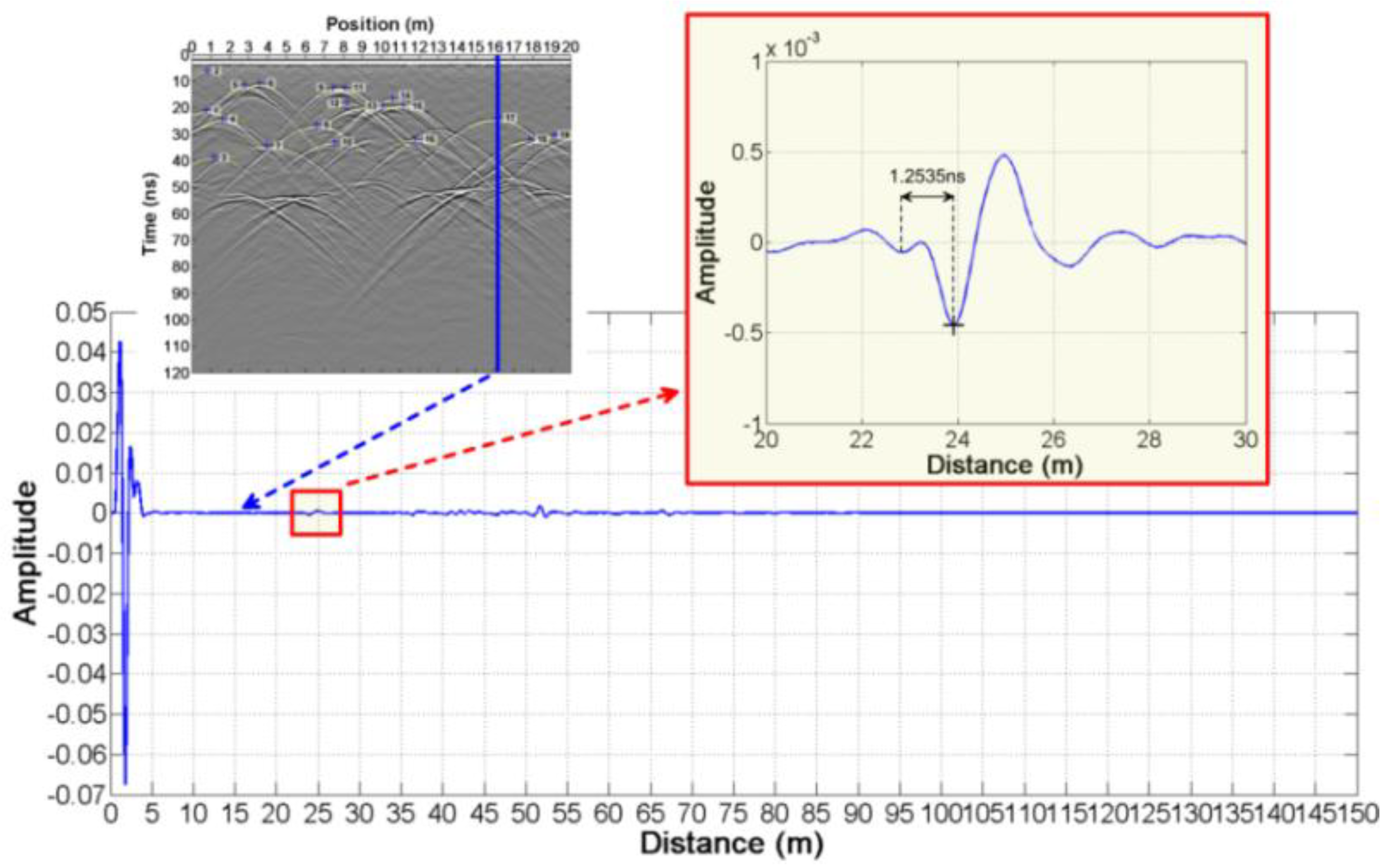
Figure 10.
The reflection wavelet waveform of the abnormal body in the complex test model.

Figure 11.
Yutu’s path on the Moon. The context image was taken by the descent camera on the CE-3 lander. The red star shows the landing site. The inset lines show the initial path (black dotted line) read directly from the Lunar Penetrating Radar (LPR) data and the adjusted path (red line).
Figure 11.
Yutu’s path on the Moon. The context image was taken by the descent camera on the CE-3 lander. The red star shows the landing site. The inset lines show the initial path (black dotted line) read directly from the Lunar Penetrating Radar (LPR) data and the adjusted path (red line).

Figure 12.
(a) The LPR CH-2A image and (b) The LPR CH-2B data image. N103-N209 denote the positions where the LPR was rebooted.
Figure 12.
(a) The LPR CH-2A image and (b) The LPR CH-2B data image. N103-N209 denote the positions where the LPR was rebooted.

Figure 13.
(a) Reflected waves caused by basalt blocksshown in CH-2A data and (b) Reflected waves caused by basalt blocksshown in CH-2B data.
Figure 13.
(a) Reflected waves caused by basalt blocksshown in CH-2A data and (b) Reflected waves caused by basalt blocksshown in CH-2B data.

Figure 14.
The reflection wavelet waveform of an abnormal body in LPR data.

Figure 15.
The histogram of the recovered permittivity.

Figure 16.
Analysis between permittivity and the depth. (a) Scatterplot of permittivity and depth. (b) The average estimated dielectric constant of regolith at each meter. The error bars show the standard deviation.
Figure 16.
Analysis between permittivity and the depth. (a) Scatterplot of permittivity and depth. (b) The average estimated dielectric constant of regolith at each meter. The error bars show the standard deviation.

Figure 17.
Analysis between permittivity and the location. (a) Scatterplot of permittivity and distance. (b) The average estimated dielectric constant of regolith at each 10 m. The error bars show the standard deviation.
Figure 17.
Analysis between permittivity and the location. (a) Scatterplot of permittivity and distance. (b) The average estimated dielectric constant of regolith at each 10 m. The error bars show the standard deviation.

Figure 18.
Analysis of the content of and and the location. (a) Scatterplot of the content of and and distance. (b) The average content of and every 10 m. The error bars show the standard deviation.
Figure 18.
Analysis of the content of and and the location. (a) Scatterplot of the content of and and distance. (b) The average content of and every 10 m. The error bars show the standard deviation.

Table 1.
Simulation Parameters.
| First Case | Second Case | |||
|---|---|---|---|---|
| Height | 0 m | 0.5 m | ||
| Offset | 1 m | 2 m | 1m | 2m |
| Center frequency | 500 MHz | 500 MHz | 500 MHz | 500 MHz |
| Waveform | Ricker | Ricker | Ricker | Ricker |
| Absorbing boundary | C-PML | C-PML | ||
| Discrete grid | 0.005 m × 0.005 m | 0.005 m × 0.005 m | ||
| Time step | 0.040434 ns | 0.040434 ns | ||
| Time window | 80 ns | 80 ns | ||
| Random access memory | 8.00 GB | 8.00 GB | ||
| Central Processing Unit | Intel(R) Core(TM) i5-4590 CPU @3.30GHz | |||
| Time | 4.5371 h | 4.6237 h | 4.5825 h | 4.6333 h |
Table 2.
Simulation parametersof the experiment models.
| Simple Model | Complex Model | |||
|---|---|---|---|---|
| Height | 0.5 m | 0.3 m | ||
| Offset | 1 m | 2 m | 0.16m | 0.32m |
| Center frequency | 500 MHz | 500 MHz | 500 MHz | 500 MHz |
| Waveform | Ricker | Ricker | Ricker | Ricker |
| Absorbing boundary | C-PML | C-PML | ||
| Discrete grid | 0.005 m × 0.005 m | 0.005 m × 0.005 m | ||
| Time step | 0.040434 ns | 0.040434 ns | ||
| Time window | 120 ns | 120 ns | ||
| Random access memory | 8.00 GB | 8.00 GB | ||
| Central Processing Unit | Intel(R) Core(TM) i5-4590 CPU @3.30GHz | |||
| Time | 14.2794 h | 14.3112 h | 20.5625 h | 20.6101 h |
Table 3.
Estimated parameters of the simple experiment model.
| Number | ||||
|---|---|---|---|---|
| 1 | 42.21 | 43.22 | 3.2917 | 2.9581 |
| 2 | 71.69 | 72.33 | 5.8370 | 2.9957 |
| 3 | 19.73 | 21.51 | 1.3041 | 2.9608 |
| 4 | 60.85 | 61.58 | 4.9433 | 2.9373 |
| 5 | 31.98 | 33.27 | 2.3579 | 3.0407 |
Table 4.
Estimated parameters of the complex test model.
| Number | ||||
|---|---|---|---|---|
| 1 | 21.0257 | 21.0662 | 1.8446 | 2.0855 |
| 2 | 6.0247 | 6.1055 | 1.1901 | 2.1815 |
| 3 | 38.5337 | 38.5741 | 2.2442 | 2.6161 |
| 4 | 24.2604 | 24.3009 | 2.0058 | 2.4644 |
| 5 | 11.6046 | 11.6854 | 1.318 | 2.5777 |
| 6 | 10.8768 | 10.9172 | 1.5026 | 1.4297 |
| 7 | 34.2072 | 34.1668 | 3.0825 | 1.7297 |
| 8 | 26.4439 | 26.6056 | 2.8795 | 2.1557 |
| 9 | 12.4537 | 12.4941 | 1.057 | 1.8755 |
| 10 | 32.7516 | 32.8325 | 3.9485 | 2.0367 |
| 11 | 12.4133 | 12.4941 | 1.3554 | 2.6194 |
| 12 | 17.9527 | 18.0336 | 2.0002 | 1.8514 |
| 13 | 19.2466 | 19.3275 | 2.2046 | 1.8754 |
| 14 | 16.5375 | 16.6184 | 1.535 | 2.718 |
| 15 | 18.9231 | 18.9636 | 1.7318 | 1.8389 |
| 16 | 31.9025 | 31.9834 | 3.9499 | 2.1793 |
| 17 | 23.8965 | 24.0987 | 3.298 | 1.4519 |
| 18 | 31.8621 | 31.9429 | 3.7867 | 1.637 |
| 19 | 30.366 | 30.4064 | 3.6163 | 1.6606 |
© 2018 by the authors. Licensee MDPI, Basel, Switzerland. This article is an open access article distributed under the terms and conditions of the Creative Commons Attribution (CC BY) license (http://creativecommons.org/licenses/by/4.0/).
Share and Cite
MDPI and ACS Style
Zhang, L.; Zeng, Z.; Li, J.; Huang, L.; Huo, Z.; Wang, K.; Zhang, J. Parameter Estimation of Lunar Regolith from Lunar Penetrating Radar Data. Sensors 2018, 18, 2907. https://doi.org/10.3390/s18092907
AMA Style
Zhang L, Zeng Z, Li J, Huang L, Huo Z, Wang K, Zhang J. Parameter Estimation of Lunar Regolith from Lunar Penetrating Radar Data. Sensors. 2018; 18(9):2907. https://doi.org/10.3390/s18092907
Chicago/Turabian StyleZhang, Ling, Zhaofa Zeng, Jing Li, Ling Huang, Zhijun Huo, Kun Wang, and Jianmin Zhang. 2018. "Parameter Estimation of Lunar Regolith from Lunar Penetrating Radar Data" Sensors 18, no. 9: 2907. https://doi.org/10.3390/s18092907
Note that from the first issue of 2016, this journal uses article numbers instead of page numbers. See further details here.