Once the candidate trees were obtained, our next objective was to determine the optimal strategy for collecting noise pollution data through smartphones. To achieve this purpose, in this section we will analyze the computation time associated with each tree element, as well as its level of accuracy. Secondly, we will analyze the energy consumption required. Finally, we will present our proposal for a balanced tree in terms of computation time and energy savings.
4.2.1. Computation Time
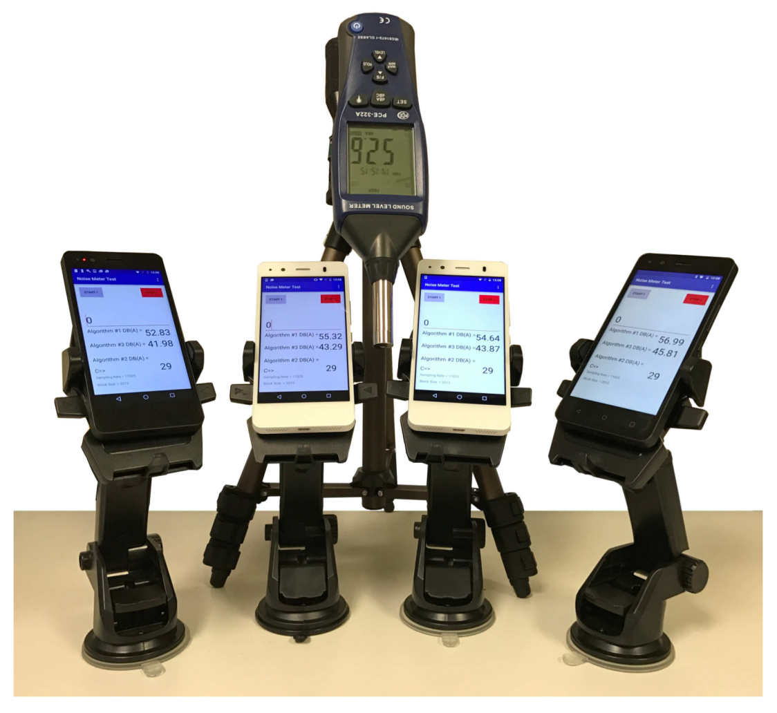
To analyze the computation time associated to each particular task, a specific application was developed to allow evaluating each attribute individually, and following a repeatable and reliable procedure. In general, 100 independent readings were obtained for each attribute to be measured, and we took their average value. A Samsung S7 Edge model running the Android 7.0.2 operating system was used for testing. Below we detail some relevant characteristics of the most critical attributes:
For the TaskDate, and TaskArea attributes, the developed application reads the data from an internal database (i.e., SQLite), and then these values were instantiated in a class for later use. We assume that the server application had previously sent these tasks to the smartphone, and so they are available for processing. In particular, the TaskArea attribute was implemented as a class that compares a polygon of n sides with the current position given by the GPS sensor. This class returns true if the smartphone is located inside such polygon.
Regarding the
Speaker, Music, and
ActiveCall, attributes, the developed application works by making calls to the corresponding API offered by the operating system. The implementation of the
PhoneStatus attribute was carried out through a service that reads the proximity, light, and accelerometer sensors. In particular, this service ends when the results are obtained. Notice that we rely on the results of a previous study [
18,
30] to determine, based on the sensor feedback, whether the smartphone is being held, it is stored in a backpack, or it is in a pocket. So, those previous results allow us to estimate the complexity of such predictions.
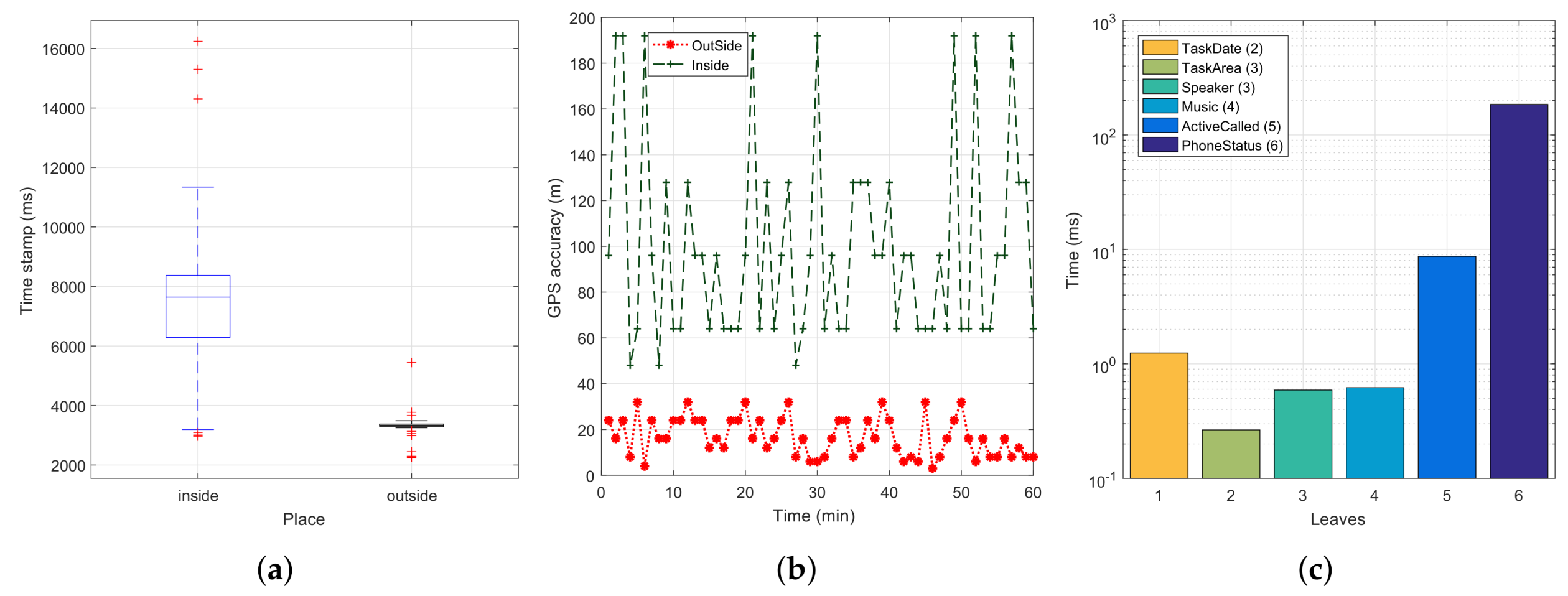
The location attribute is considered a critical factor because of its high consumption and processing time. To evaluate this attribute, we implemented a service where we read the latitude and longitude of the GPS sensor embedded in the smartphone. Also, we recorded the prediction accuracy to have a greater control of the positions obtained. A time-stamp was recorded when the GPS obtained the first coordinate. In particular, the design of our solutions aims at outdoor locations alone, meaning that we will also use the GPS to discriminate between both cases (indoor vs. outdoor). To assess the ability of the GPS sensor to differentiate between both environments, we first analyzed the accuracy results achieved inside a building (near to a window to get worst-case conditions), as well as outdoors, in an open environment. For each case, 30 records were taken at two different times: mid-morning, and mid-afternoon. Our goal is to check whether the obtained readings through our application show differentiating features for these environments.
Figure 6a shows that, in outdoor environments, 99% of the location measurements were obtained in less than 4000 ms, with just sporadic values found in the four to six seconds duration range. Besides, to ensure that the smartphone is indeed in an outdoor environment,
Figure 6b shows that a GPS accuracy (error) of 40 m or less is typically only obtainable outdoors, while indoors the accuracy (error) is typically much higher, thus allowing to discriminate between both contexts quite easily. Nevertheless, in terms of estimated error, the location API will converge to very low errors in a few seconds only when outdoors, situation where the GPS signal is available to obtain a reliable location fix. Instead, when indoors, the error cannot be reduced due to lack of GPS signal, meaning that it remains high throughout time, as only wireless networks’ data are available to provide a coarse location estimation. Hence, based on these results, we can validate the attribute location in the scope of our tree, and we will set its duration to 4000 ms, as it provides the necessary trade-off between consumption and accuracy. Finally,
Figure 6c shows the computation times associated to each key element of the tree (excluding the
Location parameter). In this Figure, it is noticeable that the
PhoneStatus attribute is the one consuming more resources in our tree, i.e., 185 ms, followed by the
ActiveCall attribute, that needs about 9 ms.
Regarding the PhoneStatus attribute, our goal was to determine, with a certain level of accuracy, whether the phone is on the user’s hand (phone either in the normal vertical position, or with left or right turn), or in a desk, but with the front facing upwards. As stated earlier, we have considered these options as the ideal moment to capture environmental noise. The idea of the different states is that there are particular user preferences when used in those positions. The capture of our training dataset was produced as shown in
Table 4, and our main goal was to determine the actual phone position: held on the hand, or at a desk facing upwards. We have developed an application to capture the different proposed states in a supervised way. The application reads the sensors: calibrated gyroscope, proximity sensor, linear acceleration, and light sensor. The capture frequency was three samples per second during one minute. After completing our learning set, the data were extracted, and we used Matlab as the tool for the handling and validation of the data.
In particular, we proceeded with the following methodology: (i) we used the K-means algorithm to classify the output from the linear acceleration sensor and the light sensor into three groups. For the linear acceleration, a single value was taken for its three axes; (ii) Once the previous classifications were obtained, a single matrix was made along with the gyroscope values in “x”, “y”, “z”, and the proximity sensor; (iii) Finally, our resulting set was processed using three different classification algorithms, and using the k-fold cross-validation on ten observations. Regarding their accuracy, MatLab shows that the Decision Tree achieves a 99.70% accuracy, while for the linear support vector machines algorithm, the accuracy achieved is slightly reduced (86.20%). The same performance occurs when using the algorithm of discrimination with a 67.90% accuracy.
Table 5 shows the confusion matrix when using the Decision Tree. We can recognize that the different states that we want to validate using our tree are clearly differentiated.
4.2.2. Energy Consumption
After determining the computation times associated with each decision attribute, we then proceeded to analyze the energy consumption of the different decisions trees. Our methodology relies on Event-based models [
27]. Specifically, a background service was implemented on the smartphone that is periodically reading the different attributes of the proposed tree; for all cases, we set the sampling period to 4 s. Before each test, we check that the smartphone’s battery is at 100%, and that Internet access is disabled. To obtain representative results, the evaluation lasted for 1 h. The smartphone used for testing is the same as above, having a battery capacity of 3600 mAh. In general, three different types of readings were made for comparison, all of them having the smartphone in the suspended mode. The situations under comparison were: (i) without the application installed; (ii) with the developed application running and testing the different attributes (but without activating the location attribute); and (iii) with the application running, but only the attribute that activates the GPS (location) is enabled. The idea of separating the location attribute from the rest is to have a better insight about the values associated with the different elements. Notice that the high amount of time and resources associated with the location attribute would blur the values related to the other attributes (typically lasting less than 200 ms), thus making such measurements less reliable and representative.
Experimental results show that the one-hour consumption estimation without the application running is of 36 mAh. Then, when turning on our developed application and running it in the background, energy consumption increases to 108 mAh. Finally, if the GPS value is obtained through the location attribute, energy consumption further raises to 180 mAh. Based on the measurements made, it was possible to assess the energy consumed (
Ah) by each attribute in our tree. The equation used for this purpose is the following:
In this equation,
represents the energy consumed during 1 s,
represents the time overhead associated with each tree attribute, and
and
represent the reference value for the energy consumed with and without the application, respectively.
N is the total number of occurrences recorded in an hour.
Table 6 summarizes the energy consumption estimation associated with each attribute on the tree. In particular, we can observe that the attributes corresponding to the GPS and PhoneStatus present the highest energy consumption values.
4.2.3. Proposed Tree and Performance Improvement
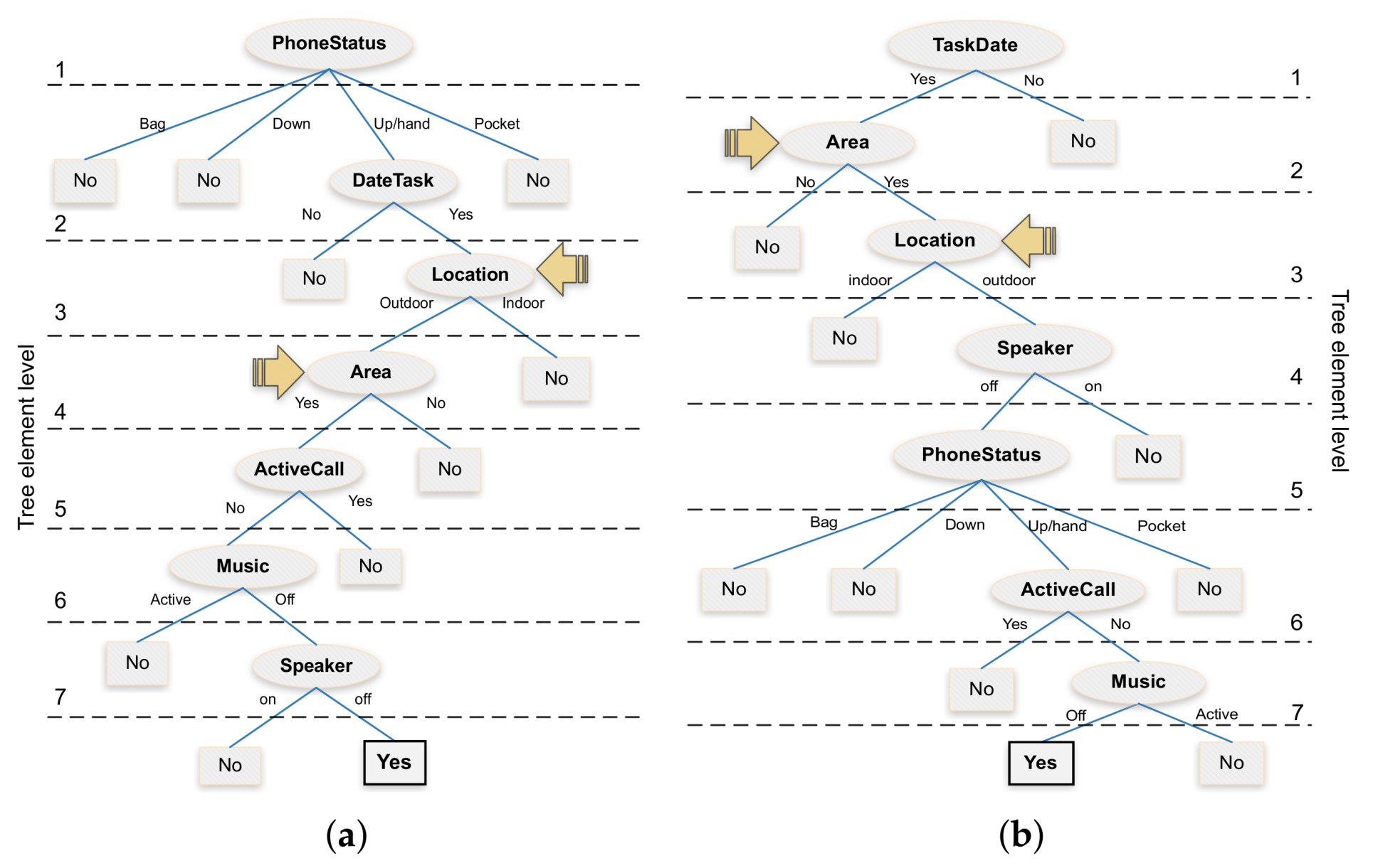
Once we obtained the computation time overhead and the energy consumption associated with each attribute, our next goal was to propose an alternative decision tree that is more resource efficient. For this purpose, we designed a tree in such a way that its elements are organized and balanced according to the desired objective of reducing time and energy overhead. In particular, for the
TaskDate,
Speaker,
Music,
ActiveCall,
PhoneStatus, and
Location attributes, we followed a sequential order by considering the computation time calculated earlier.
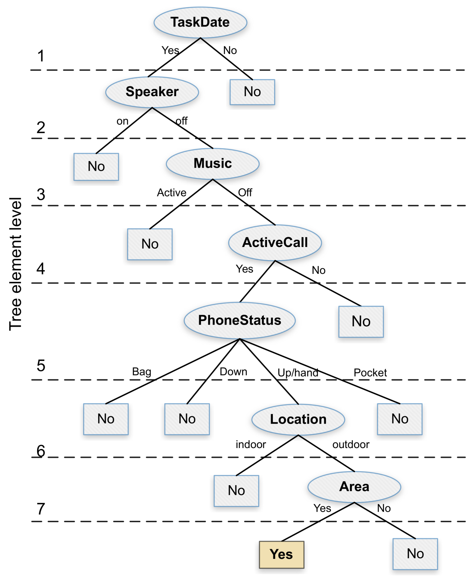
Figure 7 shows the proposed decision tree which, similarly to the J48 algorithm, can achieve a decision accuracy of 100%. Notice that, in this alternative tree, the location attribute is located near the tree bottom, thereby optimizing the overall system resources whenever a previous attribute allows discarding the noise sampling procedure by not meeting the required conditions. Besides, we can observe that the area attribute remains just below the location attribute due to its direct dependency, being this an attribute with a lower computation time, but nevertheless highly relevant in terms of the final decision.
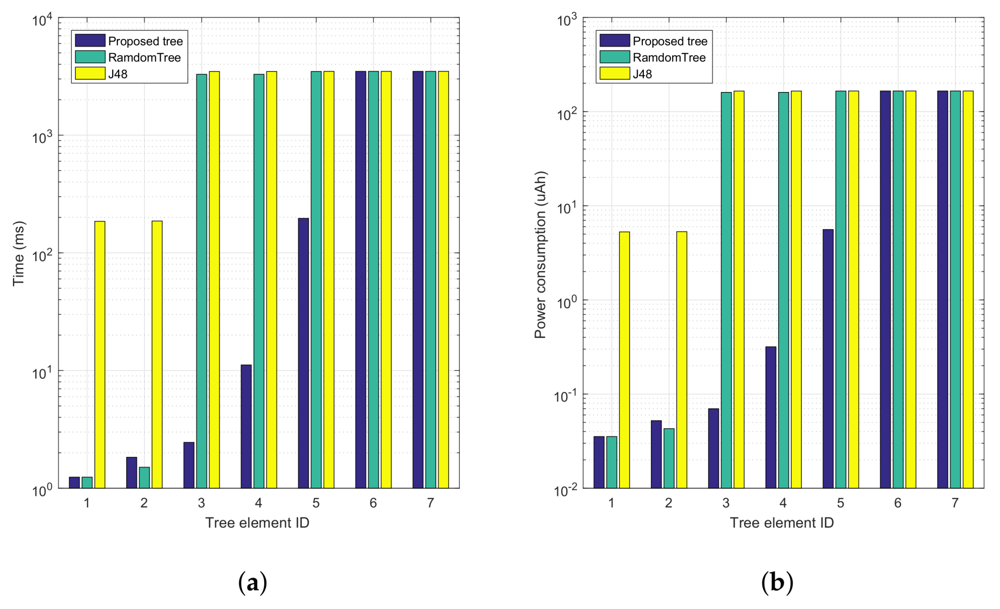
To gain further insight into the performance gains achieved,
Figure 8 shows a comparison of the accumulative computation time and energy consumption for both our proposed tree and the automatically generated trees. Increasing tree element Ids correspond to progressing along the tree, from top to bottom. In particular,
Figure 8a shows that our proposal presents a much lower time overhead compared to the two candidate trees, being that high periods of activity only take place whenever it becomes indispensable (near the bottom of the tree); specifically, the first tree elements introduce a lower time overhead compared to the others. In
Figure 8b we find a behaviour that is similar to the previous one, although it now represents the overall energy consumption associated with the proposed and automatically generated trees.
Finally,
Table 7 summarizes the performance benefits introduced by our alternative decision tree. In particular, it shows both the accumulated and average values for the time overhead and energy consumption associated with the three decision trees being compared. We find that our tree is 57.81% and 58.70% lower than the RandomTree algorithm regarding computation time and average energy consumption, respectively. For the J48 tree, improvements are further boosted by 60%, while maintaining the same decision accuracy.
Overall, we consider that the process followed in this paper to achieve a tree that is both precise and resource efficient is critical to enable the development of a crowdsensing application aiming at a widespread adoption and usage, a problem to be discussed in the next research steps.

 ,
, 


