Multiple Fusion Based on the CCD and MEMS Accelerometer for the Low-Cost Multi-Loop Optoelectronic System Control


Abstract
:1. Introduction
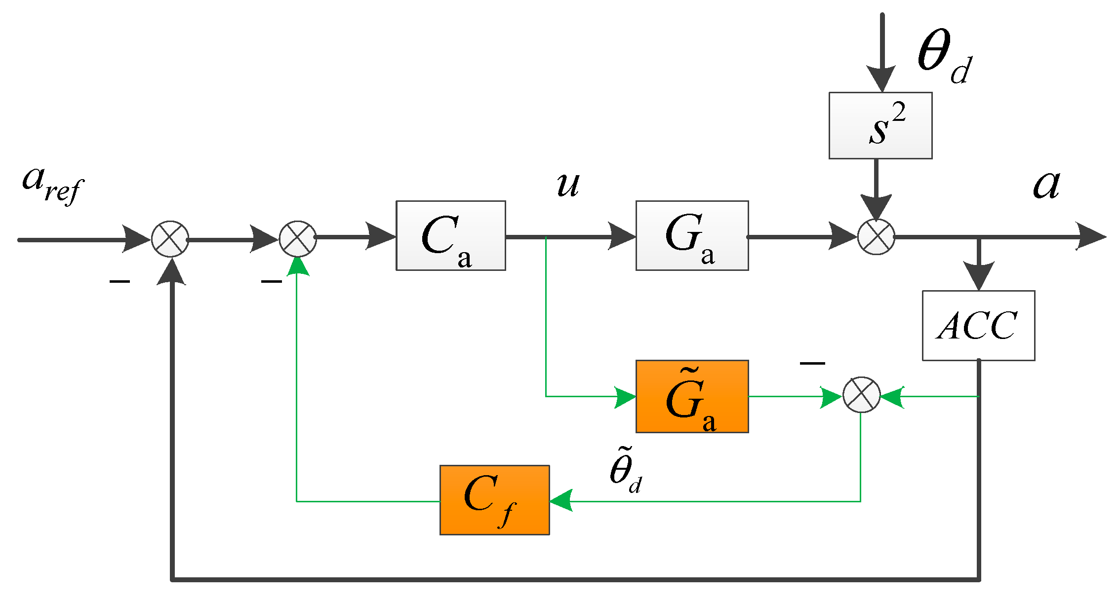
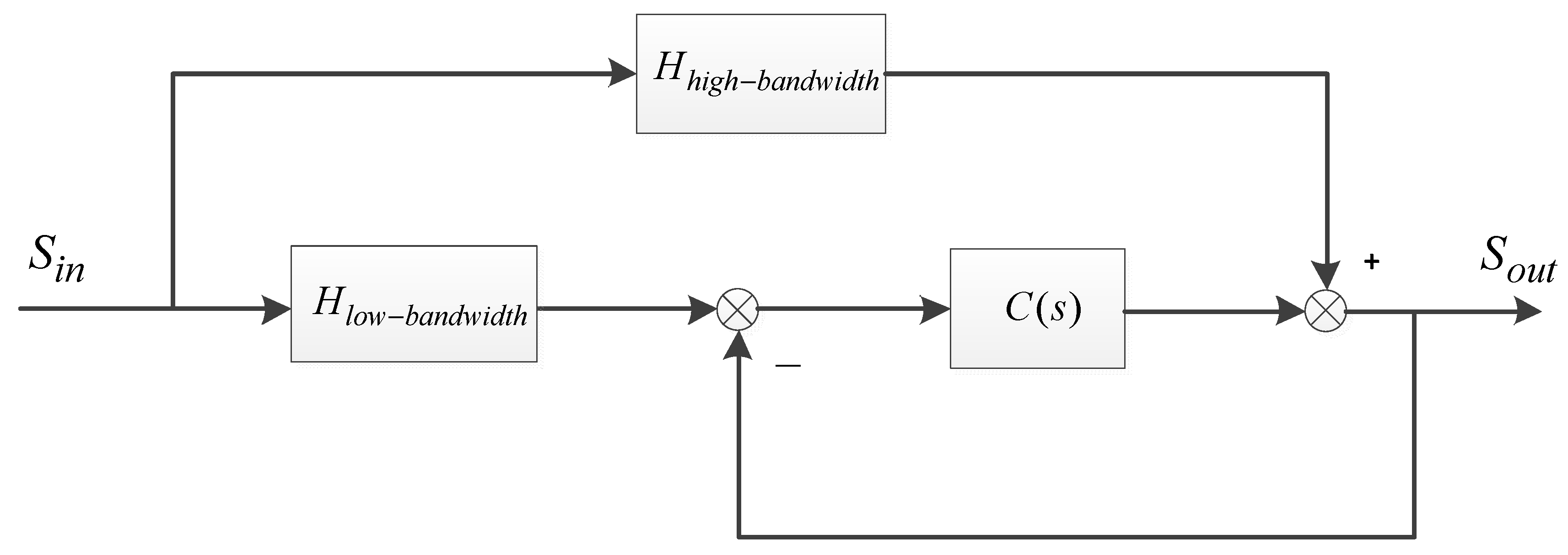
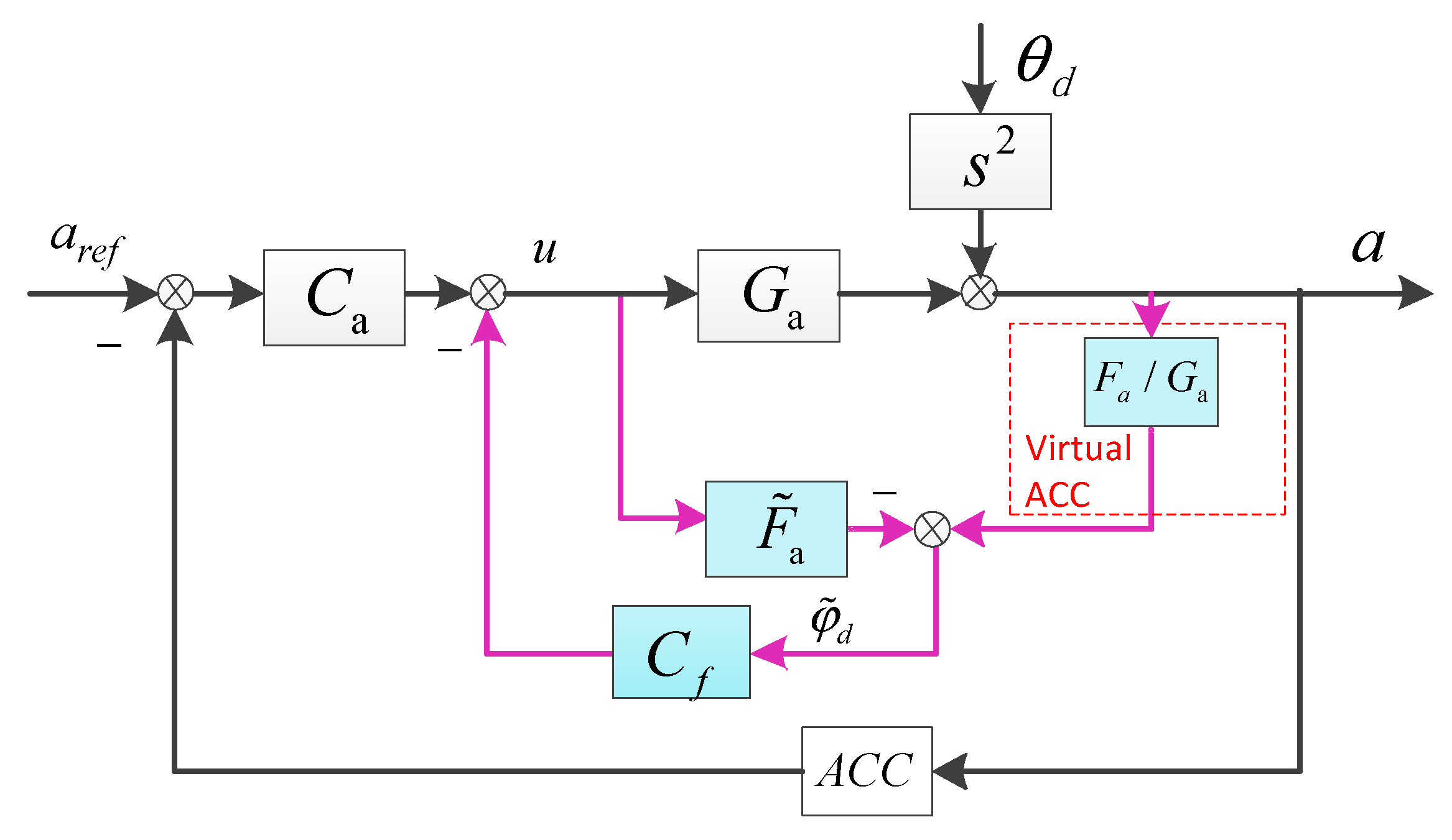
2. EDOB and FDOB
2.1. The EDOB Built in the Acceleration Control Loop
2.2. The FDOB Control
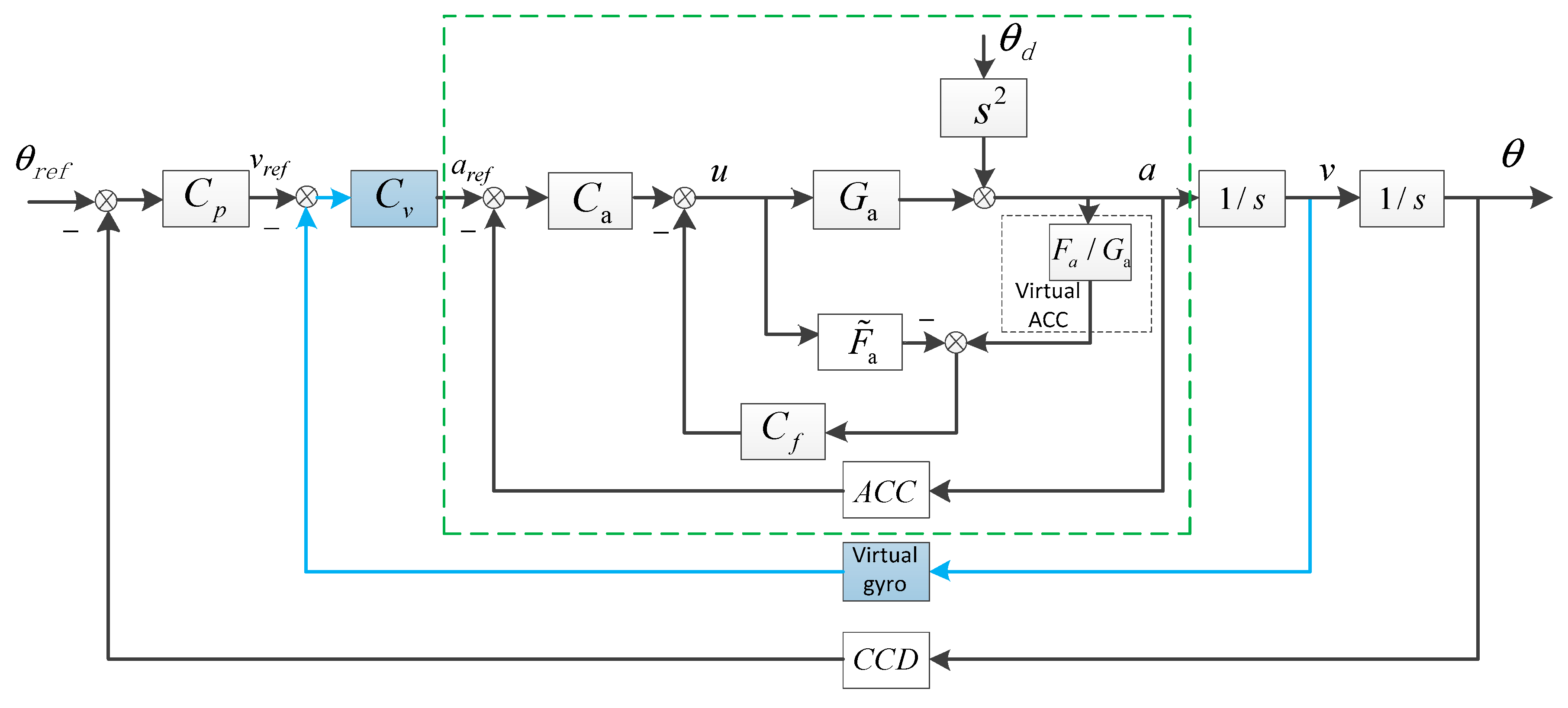
3. The Fusion Virtual Velocity Loop
4. The Complementary Filter Method and Performance Analysis
4.1. The Fusion Acceleration Based on the Modified Complementary Filter Method
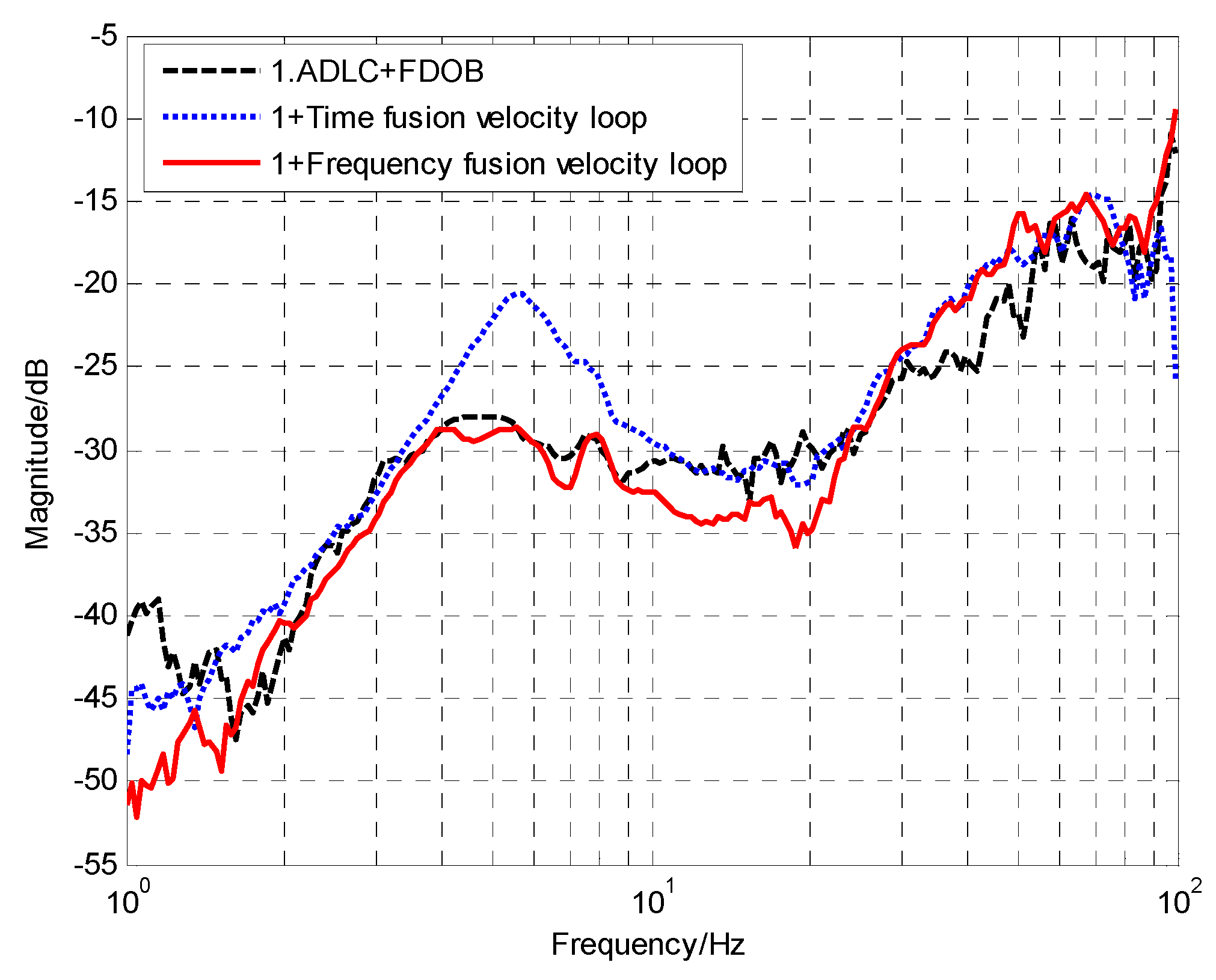
4.2. The Fusion Velocity
5. Experimental Verification
5.1. The FDOB Experiment Based on Acceleration and Position Dual-Loop Control
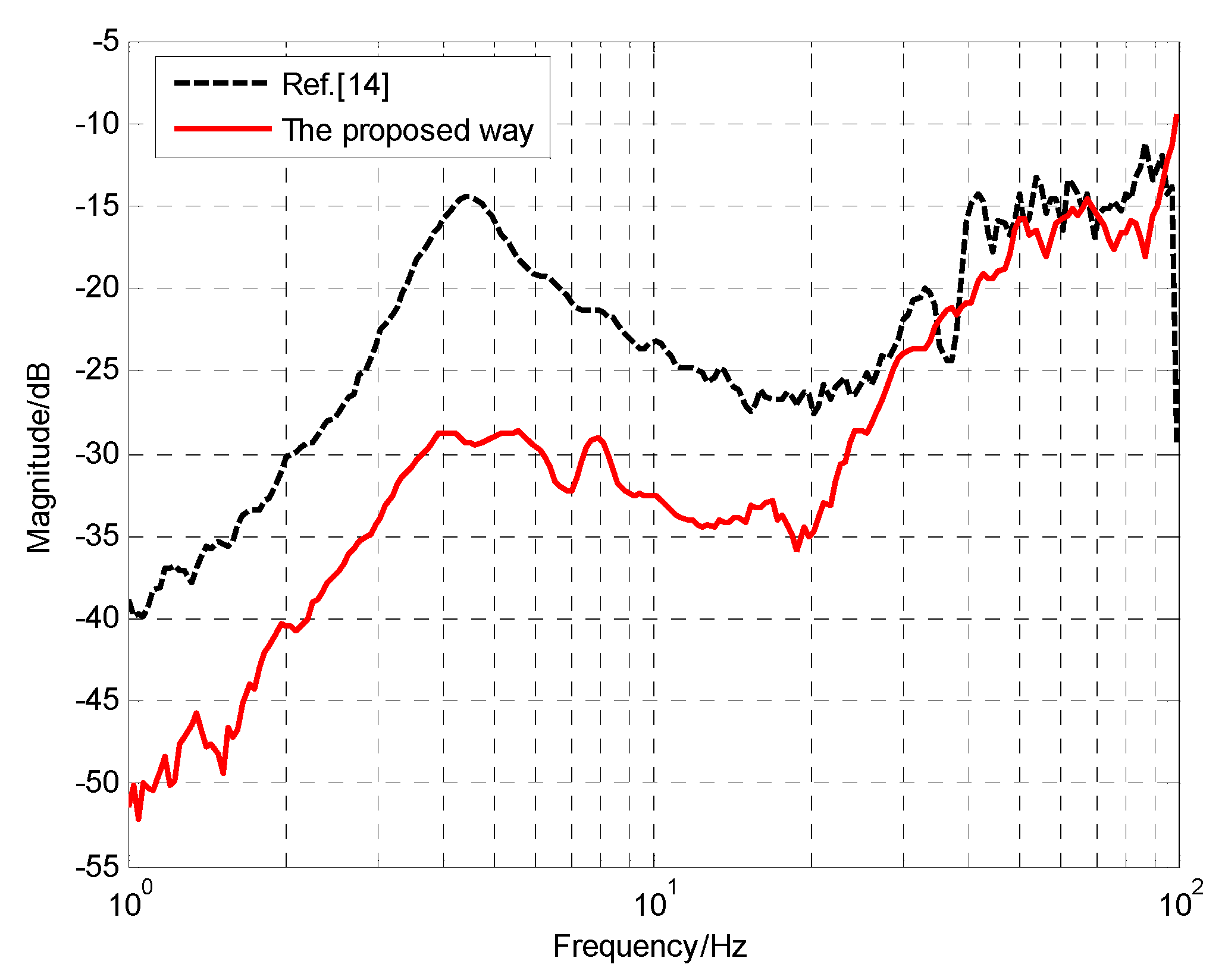
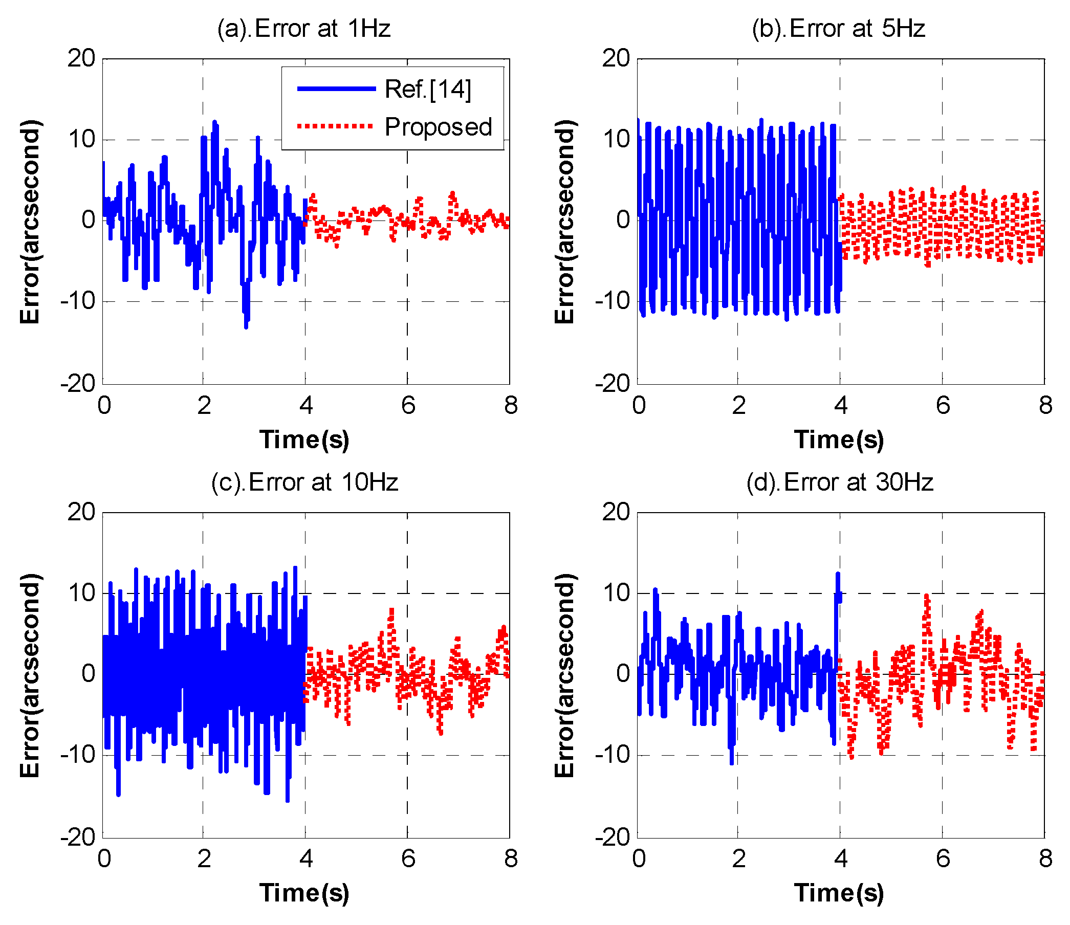
5.2. The Virtual Velocity Loop with the FDOB
6. Conclusions
Author Contributions
Funding
Acknowledgments
Conflicts of Interest
References
- Cochran, R.W.; Vassar, R.H. Fast-Steering Mirrors in Optical Control Systems. In Advances in Optical Structure Systems; The International Society for Optical Engineering: Bellingham, WA, USA, 1990; Volume 1303. [Google Scholar]
- Schneeberger, T.J.; Barker, K.W. High-altitude balloon experiment: A testbed for acquisition, tracking and pointing technologies, Optical Engineering and Photonics in Aerospace Sensing. In Acquisition, Tracking and Pointing VII; The International Society for Optical Engineering: Bellingham, WA, USA, 1993. [Google Scholar]
- Saksonov, A.; Shlomi, A.; Kopeika, N.S. Vibration noise control in laser satellite communication, Aerospace/Defense Sensing, Simulation and Controls. In Acquisition, Tracking and Pointing XV; The International Society for Optical Engineering: Bellingham, WA, USA, 2001. [Google Scholar]
- Liu, W.; Yao, K.; Huang, D.; Lin, X.; Wang, L.; Lv, Y. Performance evaluation of coherent free space optical communications with a double-stage fast-steering-mirror adaptive optics system depending on the Greenwood frequency. Opt. Express 2016, 24, 13288–13302. [Google Scholar] [CrossRef] [PubMed]
- Ekstrand, B. Tracking filters and models for seeker applications. IEEE Trans. Aerosp. Electron. Syst. 2001, 37, 965–977. [Google Scholar] [CrossRef]
- Tang, T.; Huang, Y.; Liu, S. Acceleration feedback of a CCD-based tracking loop for fast steering mirror. Opt. Eng. 2009, 48, 510–520. [Google Scholar]
- Dickson, W.C.; Yee, T.K.; Coward, J.F.; Mcclaren, A.; Pechner, D.A. Compact fiber optic gyroscopes for platform stabilization. In Nanophotonics and Macrophotonics for Space Environments VII; The International Society for Optical Engineering: Bellingham, WA, USA, 2013; pp. 7453–7458. [Google Scholar]
- Yoon, Y.G.; Lee, S.M.; Kim, J.H. Implementation of a Low-cost Fiber Optic Gyroscope for a Line-of-Sight Stabilization System. J. Inst. Control 2015, 21, 168–172. [Google Scholar] [CrossRef]
- Studenny, J.; Belanger, P.R. Robot manipulator control by acceleration feedback. In Proceedings of the 23rd IEEE Conference on Decision and Control, Las Vegas, NV, USA, 12–14 December 1984; pp. 1070–1072. [Google Scholar]
- Jager, B.D. Acceleration assisted tracking control. IEEE Control Syst. 1994, 14, 20–27. [Google Scholar] [CrossRef]
- Jing, T.; Yang, W.; Peng, Z.; Tao, T.; Li, Z. Application of MEMS Accelerometers and Gyroscopes in Fast Steering Mirror Control Systems. Sensors 2016, 16, 440. [Google Scholar]
- Wang, Q.; Cai, H.-X.; Huang, Y.-M.; Ge, L.; Tang, T.; Su, Y.-R.; Liu, X.; Li, J.-Y.; He, D.; Du, S.-P. Acceleration feedback control (AFC) enhanced by disturbance observation and compensation (DOC) for high precision tracking in telescope systems. Res. Astron. Astrophys. 2016, 16, 51–60. [Google Scholar] [CrossRef]
- Deng, C.; Yao, M.; Ren, G. MEMS Inertial Sensors-Based Multi-Loop Control Enhanced by Disturbance Observation and Compensation for Fast Steering Mirror System. Sensors 2016, 16, 1920. [Google Scholar] [CrossRef] [PubMed]
- Luo, Y.; Huang, Y.; Deng, C.; Yao, M.; Ren, W.; Wu, Q. Combining a Disturbance Observer with Triple-Loop Control Based on MEMS Accelerometers for Line-of-Sight Stabilization. Sensors 2017, 17, 2648. [Google Scholar] [CrossRef] [PubMed]
- Algrain, M.C.; Woehrer, M.K. Determination of attitude jitter in small satellites. In Acquisition Tracking & Pointing X; The International Society for Optical Engineering: Bellingham, WA, USA, 1995; pp. 215–228. [Google Scholar]
- Madgwick, S.O.H.; Harrison, A.J.L.; Vaidyanathan, R. Estimation of IMU and MARG orientation using a gradient descent algorithm. In Proceedings of the IEEE International Conference on Rehabilitation Robotics, Zurich, Switzerland, 29 June–1 July 2011; p. 5975346. [Google Scholar]
- Leong, P.H.; Arulampalam, S.; Lamahewa, T.A.; Abhayapala, T.D. A Gaussian-Sum Based Cubature Kalman Filter for Bearings-Only Tracking. IEEE Trans. Aerosp. Electron. Syst. 2013, 49, 1161–1176. [Google Scholar] [CrossRef]
- Jeon, S.; Tomizuka, M. Benefits of acceleration measurement in velocity estimation and motion control. Control Eng. Pract. 2007, 15, 325–332. [Google Scholar] [CrossRef]
- Ito, K.; Antonello, R.; Oboe, R. Performance improvement of motion control systems with low resolution position sensors using MEMS accelerometers. In Proceedings of the 39th Annual Conference of the IEEE Industrial Electronics Society (IECON 2013), Vienna, Austria, 10–13 November 2013; pp. 1–6. [Google Scholar]
- Shim, H.; Jo, N.H. An almost necessary and sufficient condition for robust stability of closed-loop systems with disturbance observer. Automatica 2009, 45, 296–299. [Google Scholar] [CrossRef]
- Yang, Z.J.; Fukushima, Y.; Qin, P. Decentralized Adaptive Robust Control of Robot Manipulators Using Disturbance Observers. IEEE Trans. Control Syst. Technol. 2012, 20, 1357–1365. [Google Scholar] [CrossRef]
- Deng, C.; Tang, T.; Mao, Y.; Ren, G. Enhanced Disturbance Observer based on Acceleration Measurement for Fast Steering Mirror Systems. IEEE Photonics J. 2017, 9. [Google Scholar] [CrossRef]


© 2018 by the authors. Licensee MDPI, Basel, Switzerland. This article is an open access article distributed under the terms and conditions of the Creative Commons Attribution (CC BY) license (http://creativecommons.org/licenses/by/4.0/).
Share and Cite
Luo, Y.; Mao, Y.; Ren, W.; Huang, Y.; Deng, C.; Zhou, X. Multiple Fusion Based on the CCD and MEMS Accelerometer for the Low-Cost Multi-Loop Optoelectronic System Control. Sensors 2018, 18, 2153. https://doi.org/10.3390/s18072153
Luo Y, Mao Y, Ren W, Huang Y, Deng C, Zhou X. Multiple Fusion Based on the CCD and MEMS Accelerometer for the Low-Cost Multi-Loop Optoelectronic System Control. Sensors. 2018; 18(7):2153. https://doi.org/10.3390/s18072153
Chicago/Turabian StyleLuo, Yong, Yao Mao, Wei Ren, Yongmei Huang, Chao Deng, and Xi Zhou. 2018. "Multiple Fusion Based on the CCD and MEMS Accelerometer for the Low-Cost Multi-Loop Optoelectronic System Control" Sensors 18, no. 7: 2153. https://doi.org/10.3390/s18072153
APA StyleLuo, Y., Mao, Y., Ren, W., Huang, Y., Deng, C., & Zhou, X. (2018). Multiple Fusion Based on the CCD and MEMS Accelerometer for the Low-Cost Multi-Loop Optoelectronic System Control. Sensors, 18(7), 2153. https://doi.org/10.3390/s18072153