Deep Learning to Predict Falls in Older Adults Based on Daily-Life Trunk Accelerometry

 ,
,  , and
, and
Abstract
1. Introduction
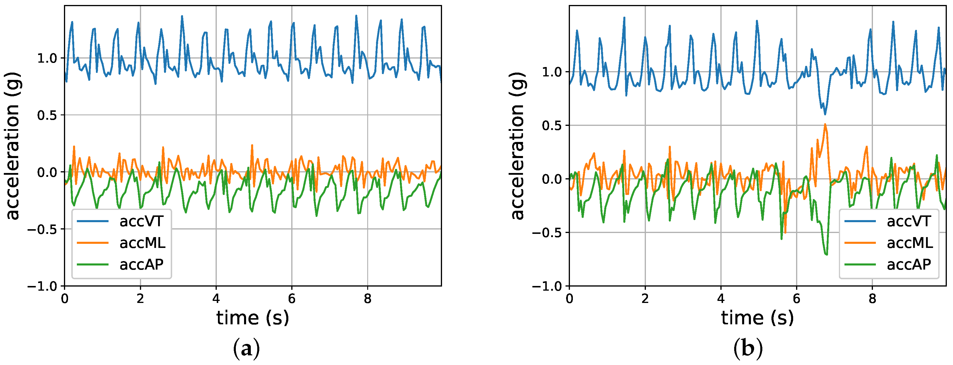
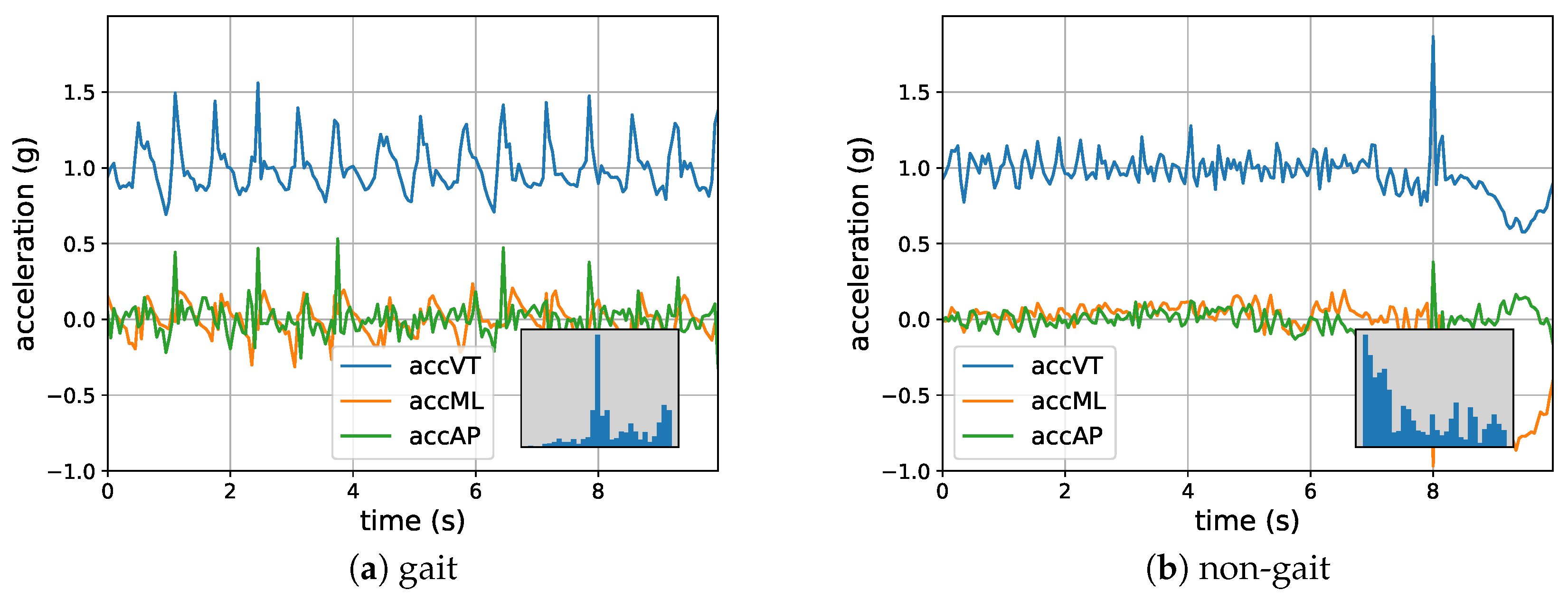
2. Sensor Data
3. Approach
4. Deep Learning Neural Network Models
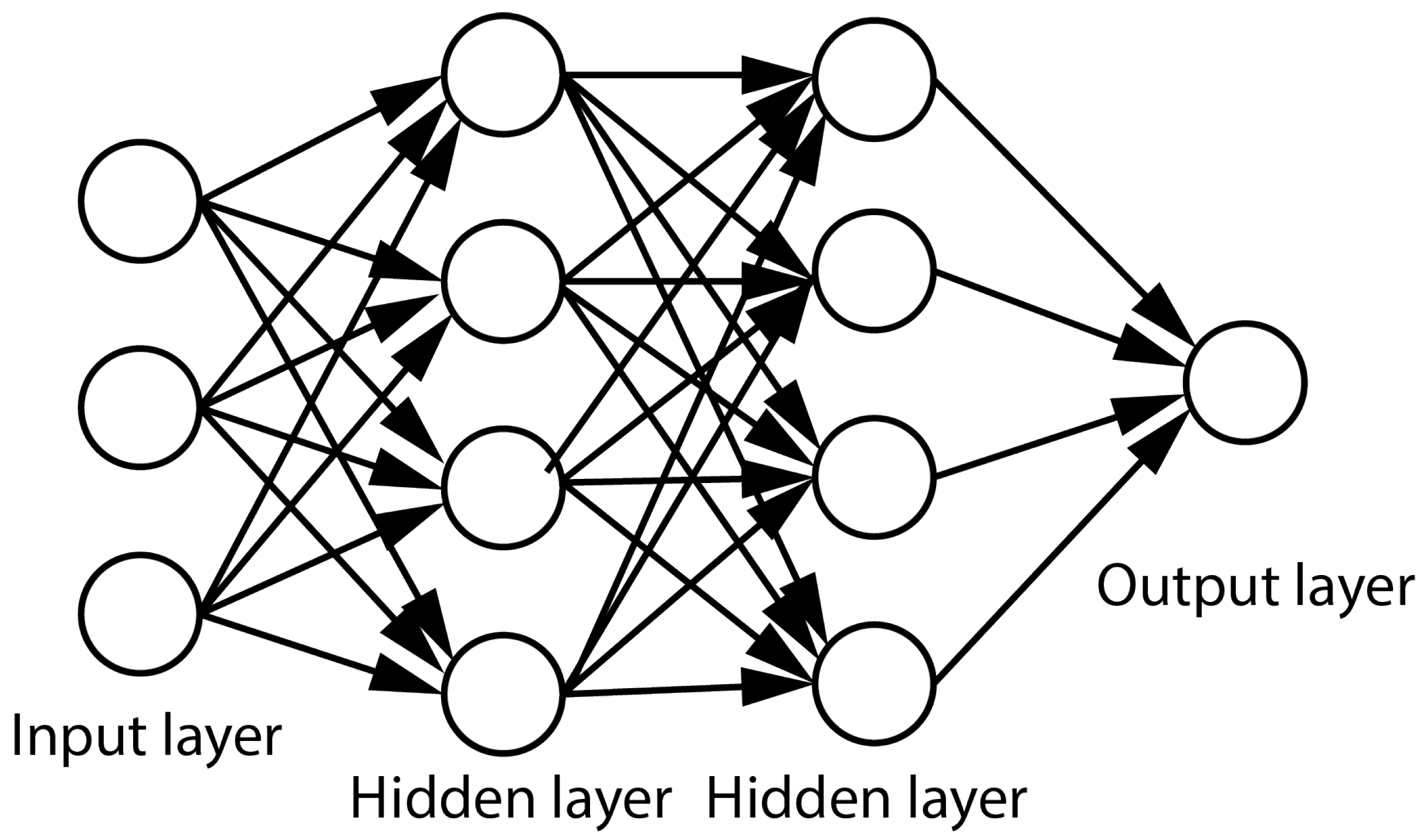
4.1. Feed-Forward Neural Networks
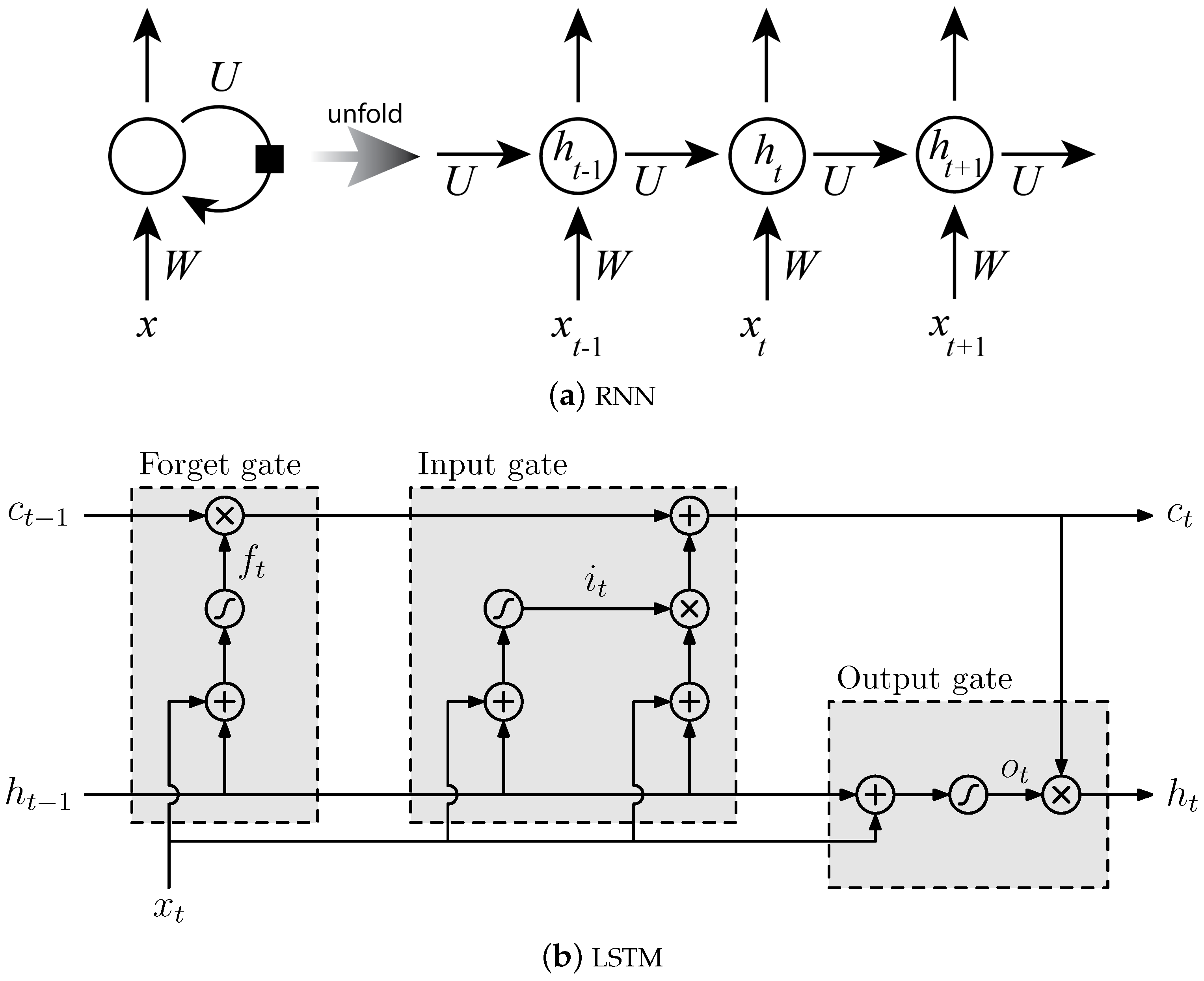
4.2. Long Short-Term Memory (LSTM) Network
4.3. Multi-Task Learning
5. Experiments and Results
5.1. Experiment 1
5.2. Experiment 2
5.3. Experiment 3
5.4. Experiment 4
5.5. Experiment 5
6. Discussion and Conclusions
Author Contributions
Acknowledgments
Conflicts of Interest
References
- Ambrose, A.F.; Paul, G.; Hausdorff, J.M. Risk factors for falls among older adults: A review of the literature. Maturitas 2013, 75, 51–61. [Google Scholar] [CrossRef] [PubMed]
- Rubenstein, L.Z. Falls in older people: Epidemiology, risk factors and strategies for prevention. Age Ageing 2006, 35, ii37–ii41. [Google Scholar] [CrossRef] [PubMed]
- Deandrea, S.; Lucenteforte, E.; Bravi, F.; Foschi, R.; La Vecchia, C.; Negri, E. Review Article: Risk Factors for Falls in Community-dwelling Older People: A Systematic Review and Meta-analysis. Epidemiology 2010, 21, 658–668. [Google Scholar] [CrossRef] [PubMed]
- Podsiadlo, D.; Richardson, S. The Timed Up & Go: A Test of Basic Functional Mobility for Frail Elderly Persons. J. Am. Geriatr. Soc. 1991, 39, 142–148. [Google Scholar] [PubMed]
- Tinetti, M.E. Performance-Oriented Assessment of Mobility Problems in Elderly Patients. J. Am. Geriatr. Soc. 1986, 34, 119–126. [Google Scholar] [CrossRef] [PubMed]
- Berg, K.O.; Wood-Dauphinee, S.L.; Williams, J.I.; Maki, B. Measuring balance in the elderly: Validation of an instrument. Physiother. Can. 1989, 41, 304–311. [Google Scholar] [CrossRef]
- Barry, E.; Galvin, R.; Keogh, C.; Horgan, F.; Fahey, T. Is the Timed Up and Go test a useful predictor of risk of falls in community dwelling older adults: A systematic review and meta-analysis. BMC Geriatr. 2014, 14, 14. [Google Scholar] [CrossRef] [PubMed]
- Ordonez, F.; Englebienne, G.; de Toledo, P.; van Kasteren, T.; Sanchis, A.; Kröse, B. Bayesian Inference in Hidden Markov Models for In-Home Activity Recognition. IEEE Pervasive Comput. 2014, 13, 67–75. [Google Scholar] [CrossRef]
- Nait Aicha, A.; Englebienne, G.; Kröse, B. Continuous measuring of the indoor walking speed of older adults living alone. J. Ambient Intell. Hum. Comput. 2017, 1–11. [Google Scholar] [CrossRef]
- Howcroft, J.; Kofman, J.; Lemaire, E.D. Review of fall risk assessment in geriatric populations using inertial sensors. J. Neuroeng. Rehabil. 2013, 10, 91. [Google Scholar] [CrossRef] [PubMed]
- Van Schooten, K.S.; Pijnappels, M.; Rispens, S.M.; Elders, P.J.; Lips, P.; van Dieën, J.H. Ambulatory fall-risk assessment: Amount and quality of daily-life gait predict falls in older adults. J. Gerontol. Ser. A Biomed. Sci. Med. Sci. 2015, 70, 608–615. [Google Scholar] [CrossRef] [PubMed]
- Rispens, S.M.; van Schooten, K.S.; Pijnappels, M.; Daffertshofer, A.; Beek, P.J.; van Dieën, J.H. Identification of fall risk predictors in daily life measurements: Gait characteristics’ reliability and association with self-reported fall history. Neurorehabil. Neural Repair 2015, 29, 54–61. [Google Scholar] [CrossRef] [PubMed]
- Weiss, A.; Brozgol, M.; Dorfman, M.; Herman, T.; Shema, S.; Giladi, N.; Hausdorff, J.M. Does the evaluation of gait quality during daily life provide insight into fall risk? A novel approach using 3-day accelerometer recordings. Neurorehabil. Neural Repair 2013, 27, 742–752. [Google Scholar] [CrossRef] [PubMed]
- Mancini, M.; Schlueter, H.; El-Gohary, M.; Mattek, N.; Duncan, C.; Kaye, J.; Horak, F.B. Continuous monitoring of turning mobility and its association to falls and cognitive function: A pilot study. J. Gerontol. Ser. A Biol. Sci. Med. Sci. 2016, 71, 1102–1108. [Google Scholar] [CrossRef] [PubMed]
- Najafi, B.; Aminian, K.; Loew, F.; Blanc, Y.; Robert, P.A. Measurement of stand-sit and sit-stand transitions using a miniature gyroscope and its application in fall risk evaluation in the elderly. IEEE Trans. Biomed. Eng. 2002, 49, 843–851. [Google Scholar] [CrossRef] [PubMed]
- Ordónez, F.J.; Roggen, D. Deep convolutional and lstm recurrent neural networks for multimodal wearable activity recognition. Sensors 2016, 16, 115. [Google Scholar] [CrossRef] [PubMed]
- Hu, B.; Dixon, P.; Jacobs, J.; Dennerlein, J.; Schiffman, J. Machine learning algorithms based on signals from a single wearable inertial sensor can detect surface-and age-related differences in walking. J. Biomech. 2018, 71, 37–42. [Google Scholar] [CrossRef] [PubMed]
- Folstein, M.F.; Folstein, S.E.; McHugh, P.R. Mini-mental state: A practical method for grading the cognitive state of patients for the clinician. J. Psychiatr. Res. 1975, 12, 189–198. [Google Scholar] [CrossRef]
- Rispens, S.M.; van Schooten, K.S.; Pijnappels, M.; Daffertshofer, A.; Beek, P.J.; van Dieën, J.H. Do extreme values of daily-life gait characteristics provide more information about fall risk than median values? JMIR Res. Protoc. 2015, 4, e4. [Google Scholar] [CrossRef] [PubMed]
- Dijkstra, B.; Kamsma, Y.; Zijlstra, W. Detection of gait and postures using a miniaturised triaxial accelerometer-based system: Accuracy in community-dwelling older adults. Age Ageing 2010, 39, 259–262. [Google Scholar] [CrossRef] [PubMed]
- Van Schooten, K.S.; Pijnappels, M.; Rispens, S.M.; Elders, P.J.M.; Lips, P.; Daffertshofer, A.; Beek, P.J.; van Dieën, J.H. Daily-life gait quality as predictor of falls in older people: A 1-year prospective cohort study. PLoS ONE 2016, 11, e0158623. [Google Scholar] [CrossRef] [PubMed]
- LeCun, Y.; Bengio, Y.; Hinton, G. Deep learning. Nature 2015, 521, 436–444. [Google Scholar] [CrossRef] [PubMed]
- Abdel-Hamid, O.; Mohamed, A.R.; Jiang, H.; Penn, G. Applying convolutional neural networks concepts to hybrid NN-HMM model for speech recognition. In Proceedings of the 2012 IEEE International Conference on Acoustics, Speech and Signal Processing (ICASSP), Kyoto, Japan, 25–30 March 2012; pp. 4277–4280. [Google Scholar]
- Krizhevsky, A.; Sutskever, I.; Hinton, G.E. Imagenet classification with deep convolutional neural networks. In Proceedings of the 25th International Conference on Neural Information Processing Systems, Lake Tahoe, NV, USA, 3–6 December 2012; pp. 1097–1105. [Google Scholar]
- Toshev, A.; Szegedy, C. Deeppose: Human pose estimation via deep neural networks. In Proceedings of the IEEE Conference on Computer Vision and Pattern Recognition, Columbus, OH, USA, 24–27 June 2014; pp. 1653–1660. [Google Scholar]
- Sutskever, I.; Vinyals, O.; Le, Q.V. Sequence to sequence learning with neural networks. In Proceedings of the Advances in Neural Information Processing Systems, Montreal, QC, Canada, 8–13 December 2014; pp. 3104–3112. [Google Scholar]
- Graves, A. Generating sequences with recurrent neural networks. arXiv, 2013; arXiv:1308.0850. [Google Scholar]
- Bal, H.; Epema, D.; de Laat, C.; van Nieuwpoort, R.; Romein, J.; Seinstra, F.; Snoek, C.; Wijshoff, H. A Medium-Scale Distributed System for Computer Science Research: Infrastructure for the Long Term. Computer 2016, 49, 54–63. [Google Scholar] [CrossRef]
- Bengio, Y.; Simard, P.; Frasconi, P. Learning long-term dependencies with gradient descent is difficult. IEEE Trans. Neural Netw. 1994, 5, 157–166. [Google Scholar] [CrossRef] [PubMed]
- Hochreiter, S.; Schmidhuber, J. Long Short-Term Memory. Neural Comput. 1997, 9, 1735–1780. [Google Scholar] [CrossRef] [PubMed]
- Caruana, R. Multitask Learning: A Knowledge-Based Source of Inductive Bias. In Proceedings of the Tenth International Conference on Machine Learning, Amherst, MA, USA, 27–29 June 1993; pp. 41–48. [Google Scholar]
- Van Kasteren, T.L.; Englebienne, G.; Kröse, B.J. Hierarchical activity recognition using automatically clustered actions. In Proceedings of the International Joint Conference on Ambient Intelligence, Amsterdam, The Netherlands, 16–18 November 2011; pp. 82–91. [Google Scholar]


| Male (%) | Age (Years) | Weight (kg) | Height (cm) | |
|---|---|---|---|---|
| Mean | 74.1 | 75.3 | 49.2 | 170.6 |
| Standard deviation | - | 6.8 | 13.3 | 8.8 |
| 25% Quantile | - | 70.0 | 64.0 | 165.0 |
| 75% Quantile | - | 80.0 | 81.8 | 176.0 |
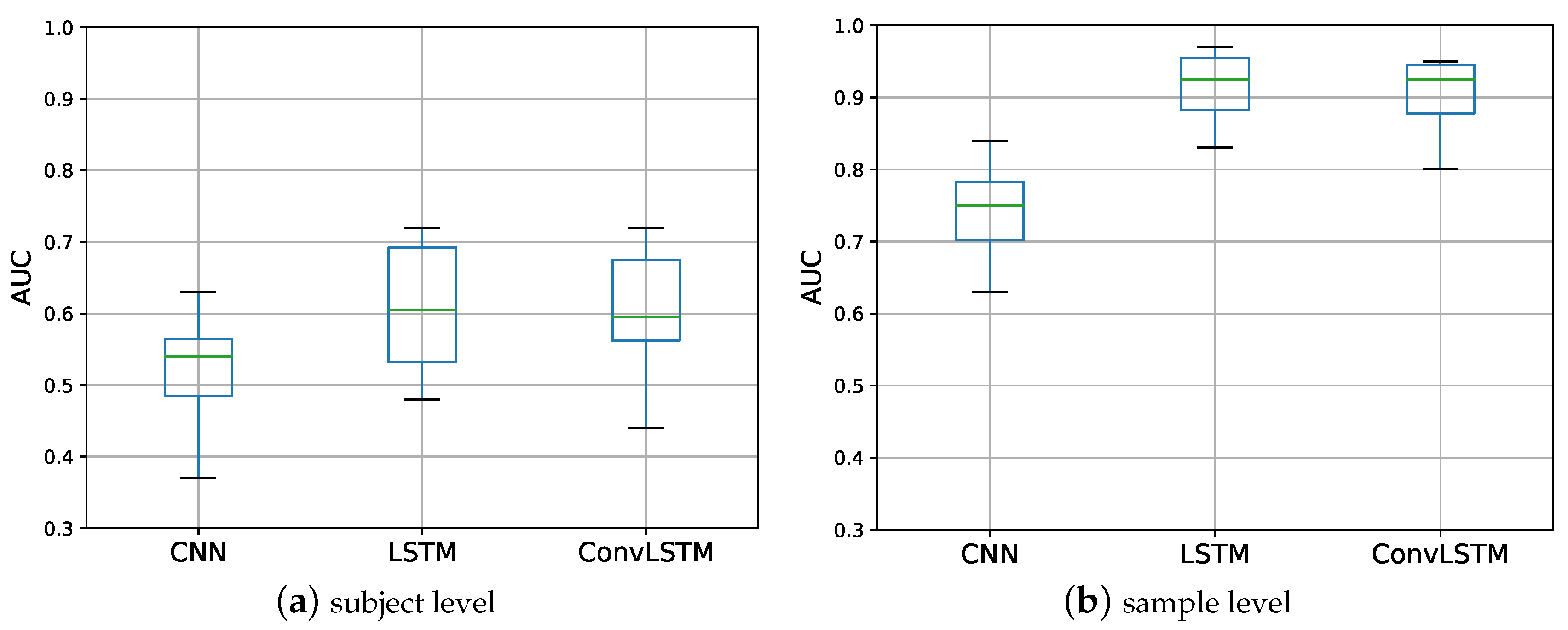
| Subject Level | Sample Level | |||
|---|---|---|---|---|
| AUC | Time (h) | AUC | Time (h) | |
| CNN | 0.52 (0.07) | 6 | 0.74 (0.07) | 7 |
| LSTM | 0.61 (0.10) | 160 | 0.91 (0.06) | 180 |
| ConvLSTM | 0.60 (0.09) | 35 | 0.90 (0.05) | 40 |
| Layer Index | 01 | 03 | 05 | 07 | 09 | 11 | 12 |
|---|---|---|---|---|---|---|---|
| type of filter | CNN | CNN | CNN | CNN | CNN | LSTM | Dense |
| number of filters | N | N | N | N | 2 |
| Dataset Size in Minutes | |||||
|---|---|---|---|---|---|
| 10 | 30 | 60 | 120 | Complete Dataset | |
| Average AUC | 0.61 | 0.63 | 0.65 | 0.65 | 0.65 |
| Training duration (h) | 35 | 90 | 150 | 250 | 350 |
| Number of folds | 10 | 10 | 10 | 2 | 1 |
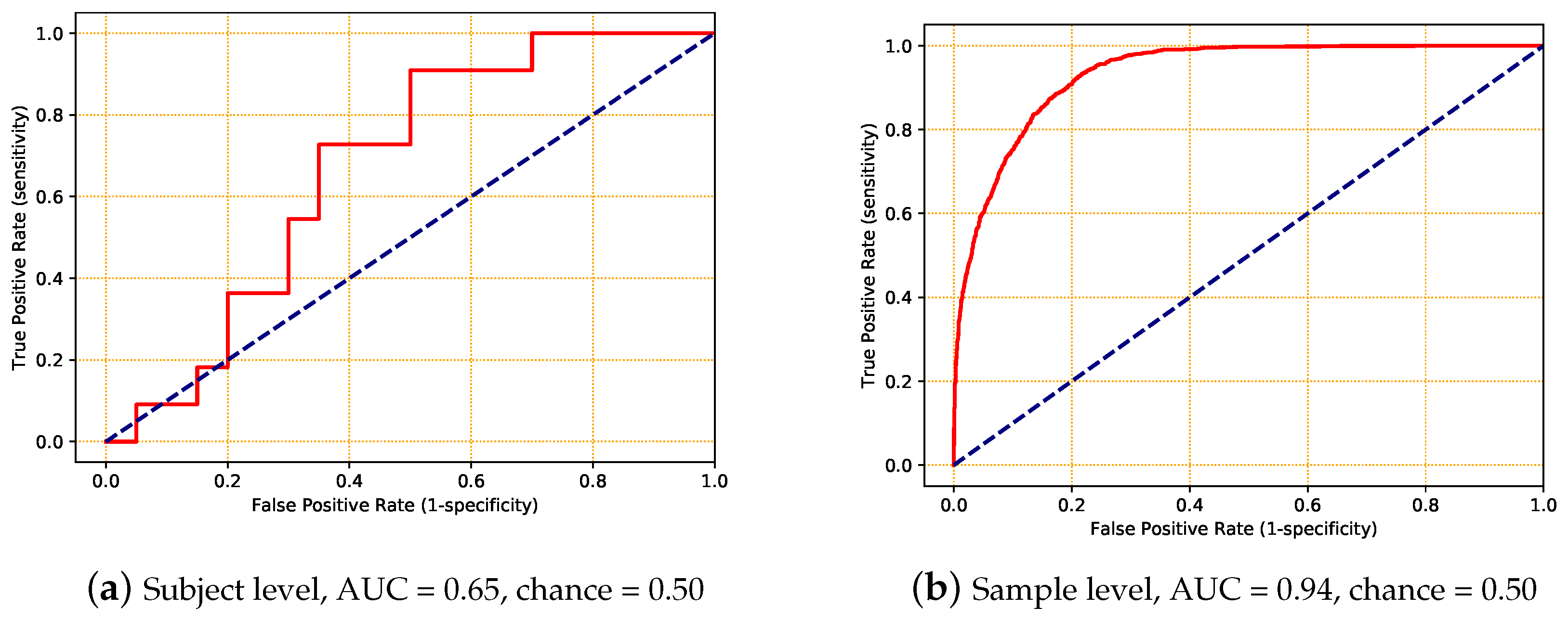
| AUC | ||
|---|---|---|
| Average | Standard Deviation | |
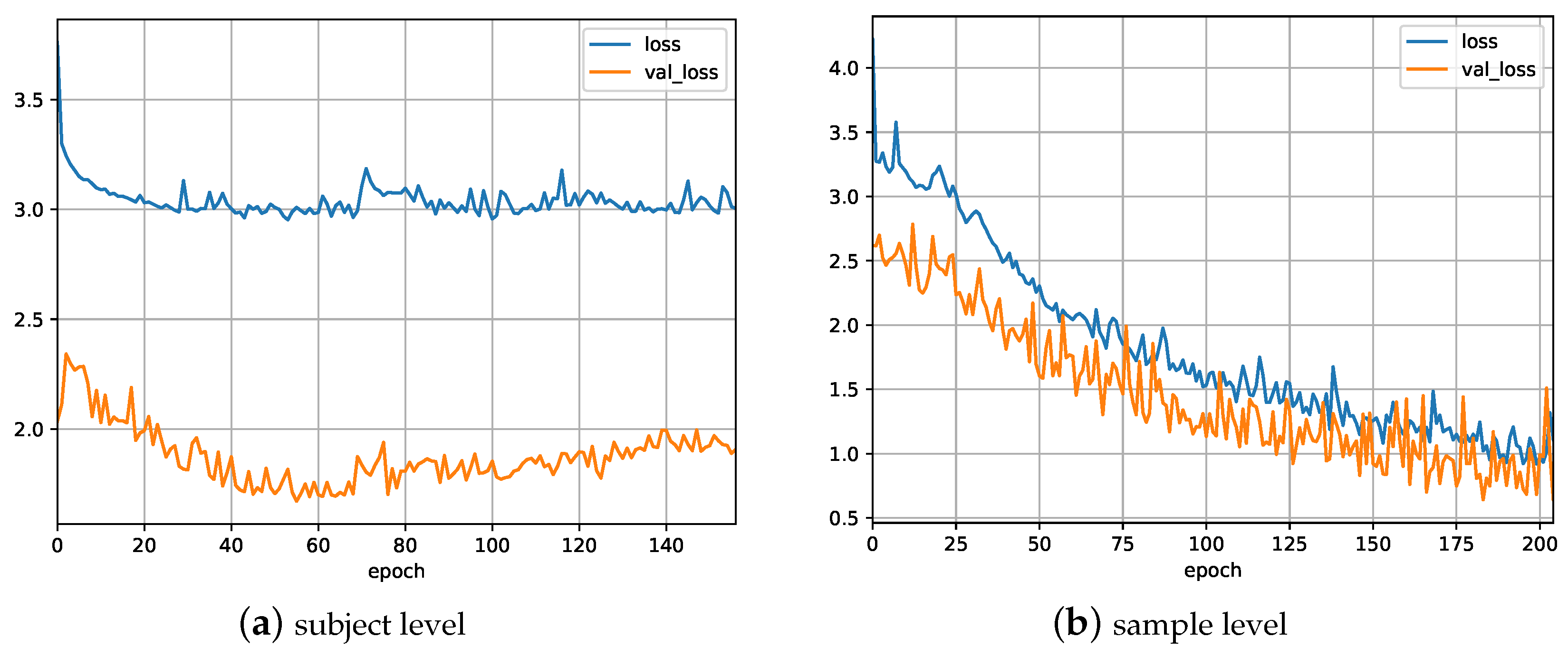
| subject level | 0.65 | 0.09 |
| sample level | 0.94 | 0.07 |
| Characteristic | AUC Main Task (std dev) | p-Value Diff to Base Model | ||
|---|---|---|---|---|
| Experiment 4 | Experiment 5 | Experiment 4 | Experiment 5 | |
| Gender | 0.70 (0.06) | 0.75 (0.05) | 0.070 | <0.001 |
| Age | 0.70 (0.05) | 0.74 (0.05) | 0.082 | <0.001 |
| Weight | 0.68 (0.05) | 0.72 (0.05) | 0.306 | 0.005 |
| Height | 0.63 (0.06) | 0.65 (0.06) | 0.987 | 0.897 |
© 2018 by the authors. Licensee MDPI, Basel, Switzerland. This article is an open access article distributed under the terms and conditions of the Creative Commons Attribution (CC BY) license (http://creativecommons.org/licenses/by/4.0/).
Share and Cite
Nait Aicha, A.; Englebienne, G.; Van Schooten, K.S.; Pijnappels, M.; Kröse, B. Deep Learning to Predict Falls in Older Adults Based on Daily-Life Trunk Accelerometry. Sensors 2018, 18, 1654. https://doi.org/10.3390/s18051654
Nait Aicha A, Englebienne G, Van Schooten KS, Pijnappels M, Kröse B. Deep Learning to Predict Falls in Older Adults Based on Daily-Life Trunk Accelerometry. Sensors. 2018; 18(5):1654. https://doi.org/10.3390/s18051654
Chicago/Turabian StyleNait Aicha, Ahmed, Gwenn Englebienne, Kimberley S. Van Schooten, Mirjam Pijnappels, and Ben Kröse. 2018. "Deep Learning to Predict Falls in Older Adults Based on Daily-Life Trunk Accelerometry" Sensors 18, no. 5: 1654. https://doi.org/10.3390/s18051654
APA StyleNait Aicha, A., Englebienne, G., Van Schooten, K. S., Pijnappels, M., & Kröse, B. (2018). Deep Learning to Predict Falls in Older Adults Based on Daily-Life Trunk Accelerometry. Sensors, 18(5), 1654. https://doi.org/10.3390/s18051654