We present and evaluate the results of the model and the testbed separately. The model results present measurements and evaluations of the sensor model itself, and its effectiveness in terms of reduced number of packet transmissions and reproducibility of the approximated sensor values based on the model parameters at the fog node. The testbed results present the features and measurements on how well the sensor network layer, fog computing layer and cloud computing layer collaborate and perform as one system. The implications of these results are discussed at the end of this section.
6.1. Sensor Data Experiments
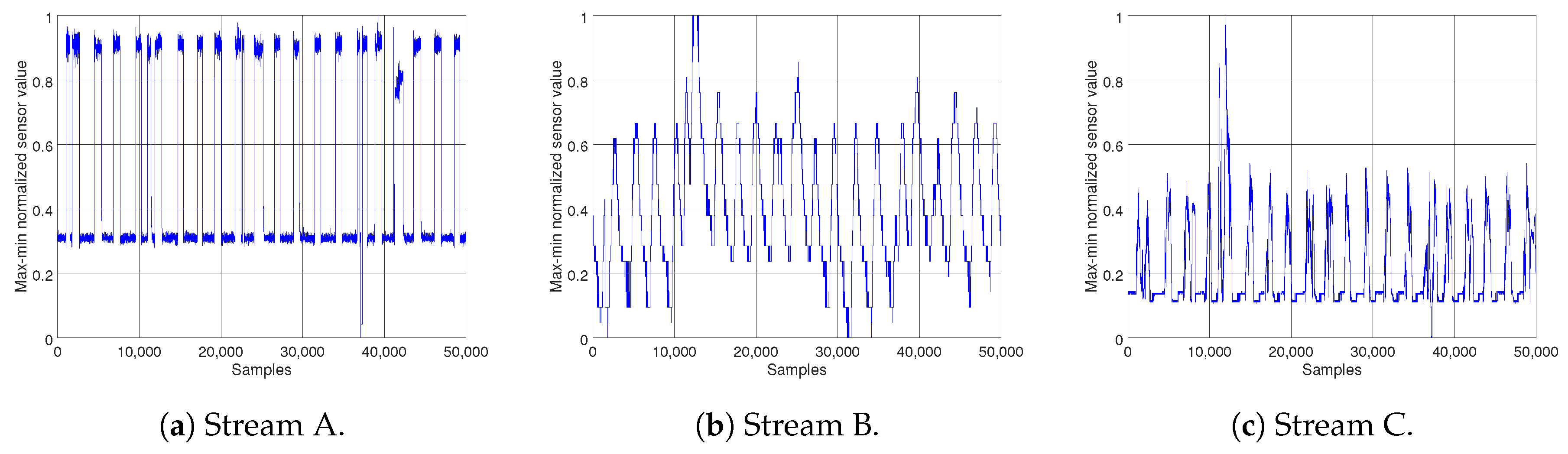
The average model performance and the reduced number of packet transmissions were measured and evaluated by implementing the proposed model in Matlab. Forty thousand continuous data points from each of the data streams were sampled.
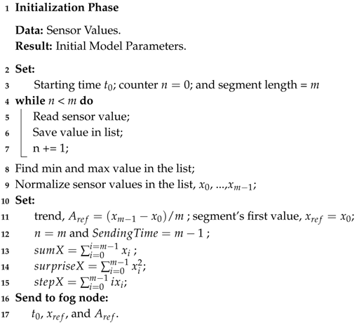
According to the model explained in
Section 3, two parameters of trend threshold
and maximum number of data points in each segment, as well as segment length
m, have the highest effect on the model performance. The reason is that they indicate the level of trade off between energy efficiency, with respect to transmission reduction, and sensitivity of the model in trend and change detection, which has a direct effect on the accuracy of the simulated data stream at the fog node. Several experiments with various values of
and
m for each of the data streams were conducted, to investigate these effects on simulation accuracy at the fog node in terms of mean square error, and to choose the most appropriate set of parameters for the model.
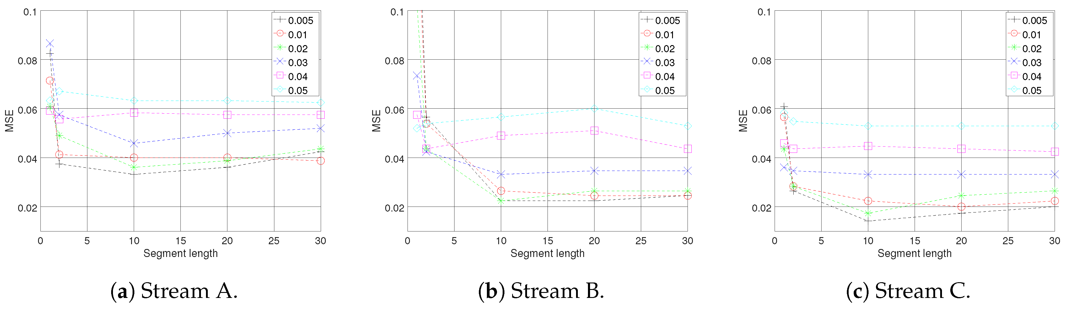
Figure 5 presents the results. As can be seen from the graphs, the mean error of the simulated data streams at the fog node has the sharpest decline for all sets of parameters, when the simulations were based on statistical information from two data points,
. From this point on the results of each of the data streams show different patterns; nonetheless, the best parameter set for all of the data streams, with respect to the MSE, was achieved by
, see
Figure 5a–c. At this point for almost all sets of parameters, the trend reversed and has raised steadily. The complete results are summarized in
Table 1.
It should be noted that, when choosing the maximum length of the segment, although a greater
m means fewer transmissions, hence achieving more energy efficiency, it also means more delay on detecting trend changes and state switches. It also indicates decreased accuracy, since the summary information would be an approximation of a larger number of data points. So although smaller values of
m might seem encouraging, for improving the energy efficiency, it is better for them to be excluded to prevent accuracy loss. Looking at
Figure 5, it can be seen that the MSE shows a fairly stable trend when segment length increases from 10 to 20, with
for stream A and
for streams B and C. For this reason, the parameter set
for streams B and C, and
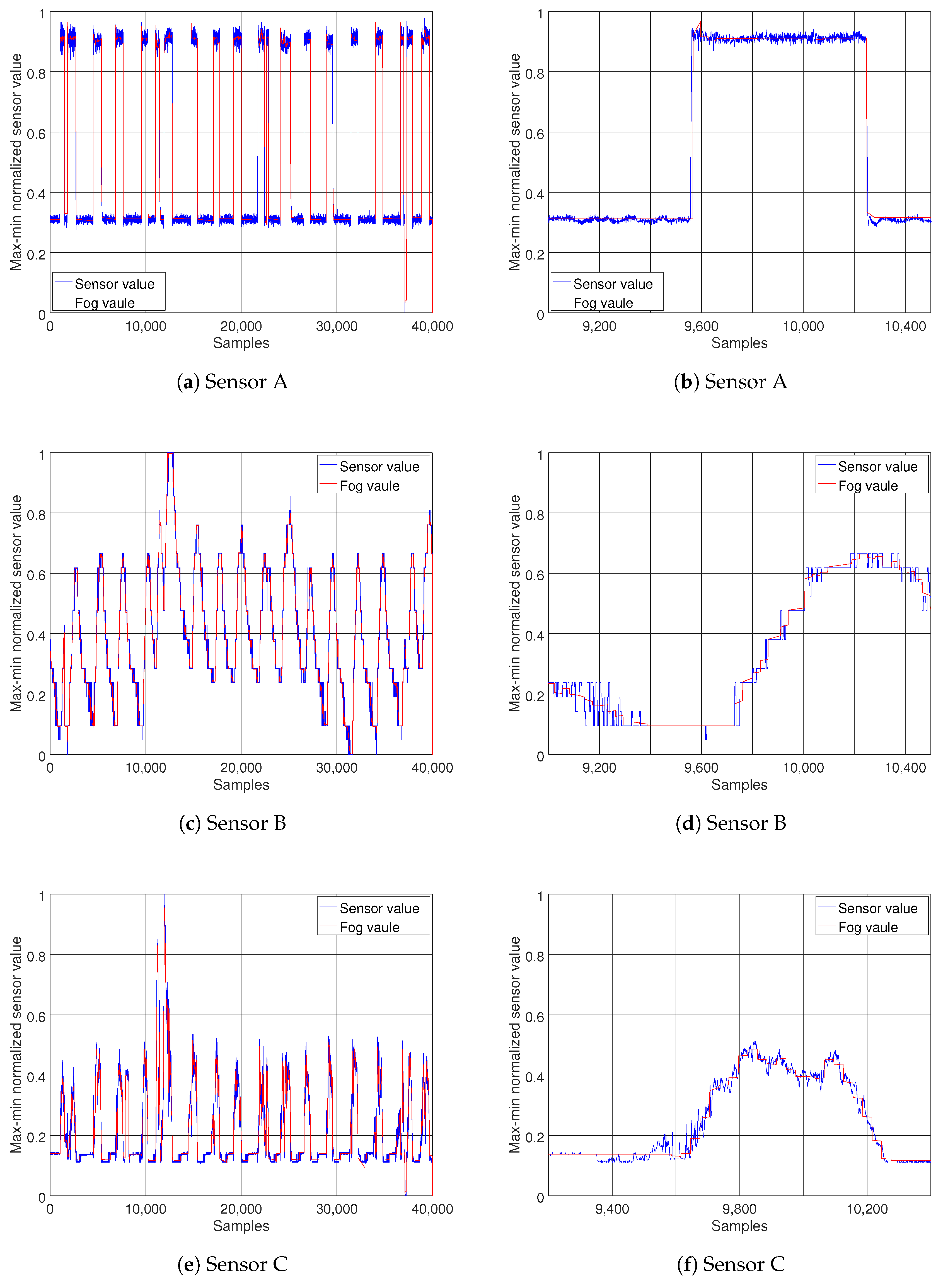
for A, were chosen to test the performance of the proposed model. After setting the model parameters, several experiments were carried out for all three data streams. The red lines on
Figure 6 show the simulated data streams at the fog node, and the blue lines illustrate the original data streams. On the left column of
Figure 6a,c,e, the results of the model for the duration of the experiment are presented. To illustrate the results in more detail,
Figure 6b,d,f show zoomed in versions of the same data streams. It is clearly observable that the model captures the behavior of the data streams with good accuracy and low delay.
For this experiment, 40,000 data points from each of the data streams were used. The number of packets sent to a fog node after deploying the model reduced to 812, 898 and 926 for A, B and C, respectively; that is a communication reduction ratio of 49 to 1, 45 to 1 and 43 to 1. In total, for all the data streams, only 2636 of the data points (from the original 120,000 data points) were transmitted. Hence, approximately 2.2% of the packets were sent from sensor devices to a fog node. To compare the performance of the proposed method, the MSE measure of the base model was obtained, with respect to the segment length, see
Table 2. As mentioned before, the best parameters set for the proposed method was
, with respect to MSE of the simulated data streams at fog node; in addition, the MSE measure was fairly stable with segment length
to
. Choosing the parameter set
, we can compare the simulation accuracy of the two models. The MSE measure of the data streams A, B, and C were 0.036, 0.022, and 0.017, respectively, when the proposed model was used to simulate the data streams at the fog node; these values for the base model were A = 0.43, B = 0.025, and C = 0.019. It is clear that the proposed method was able to simulate the data stream with a higher accuracy. In terms of transmission reduction, the proposed model simulated the data streams A, B and C with MSE of 0.038, 0.024 and 0.02, respectively, when transmitting one packet every 20 data points, with the most appropriate parameter set. For the base model to achieve the same level of accuracy, the maximum segment length cannot be more than 17 for stream A, 19 for stream B, and 23 for stream C. This means that approximately 15.5% of all the packets need to be sent, which makes the communication cost of the base model 7.5 times more than the proposed model.
Considering the presented results, it is reasonable to conclude that the proposed model can successfully reduce the number of packet transmissions, while keeping the error of the simulated data stream, using only statistical information, within an acceptable range.
6.2. Testbed Evaluation
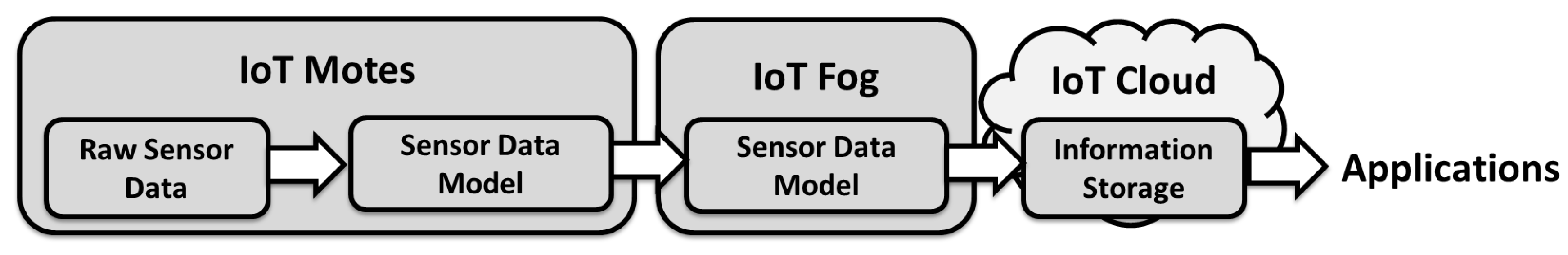
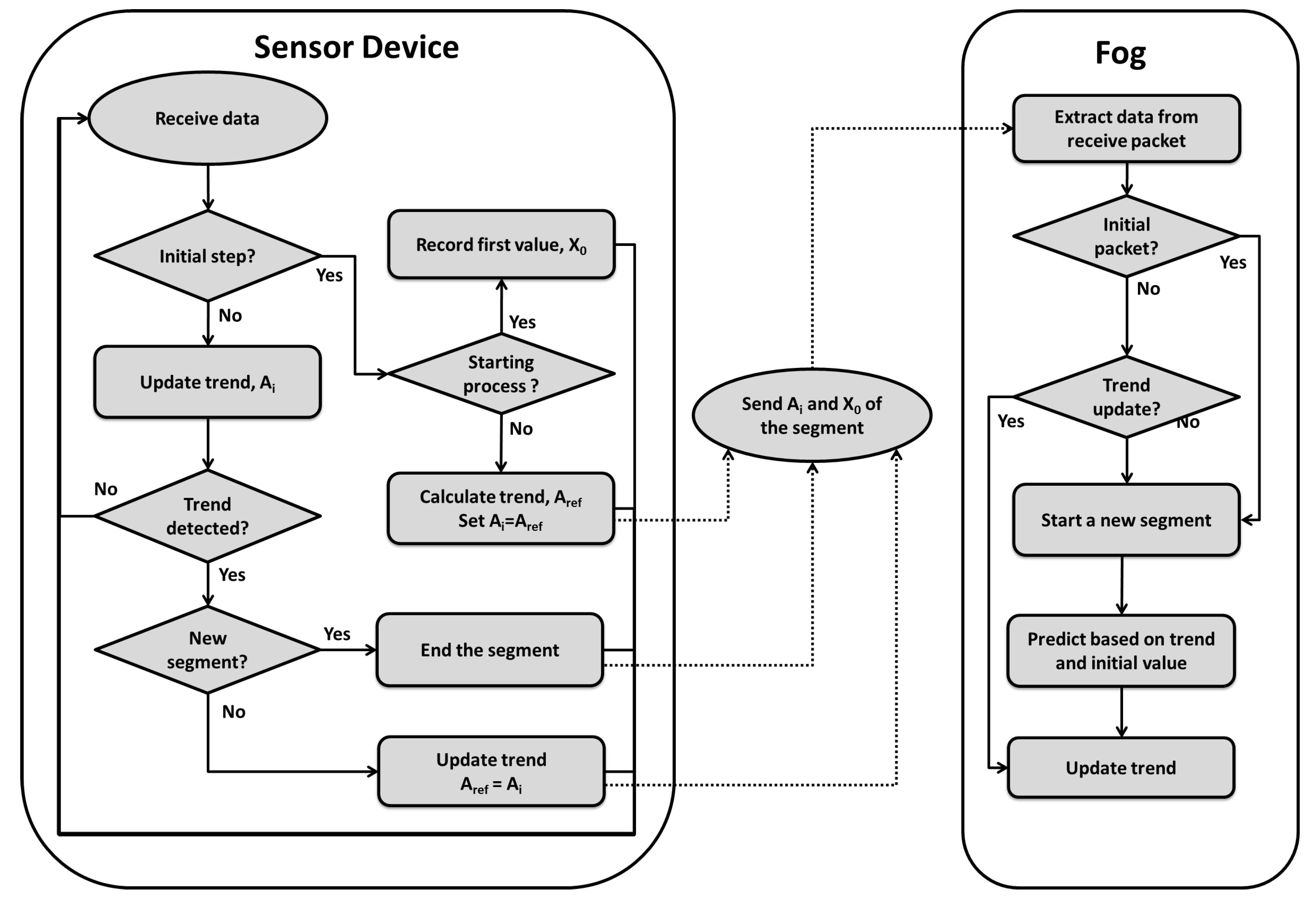
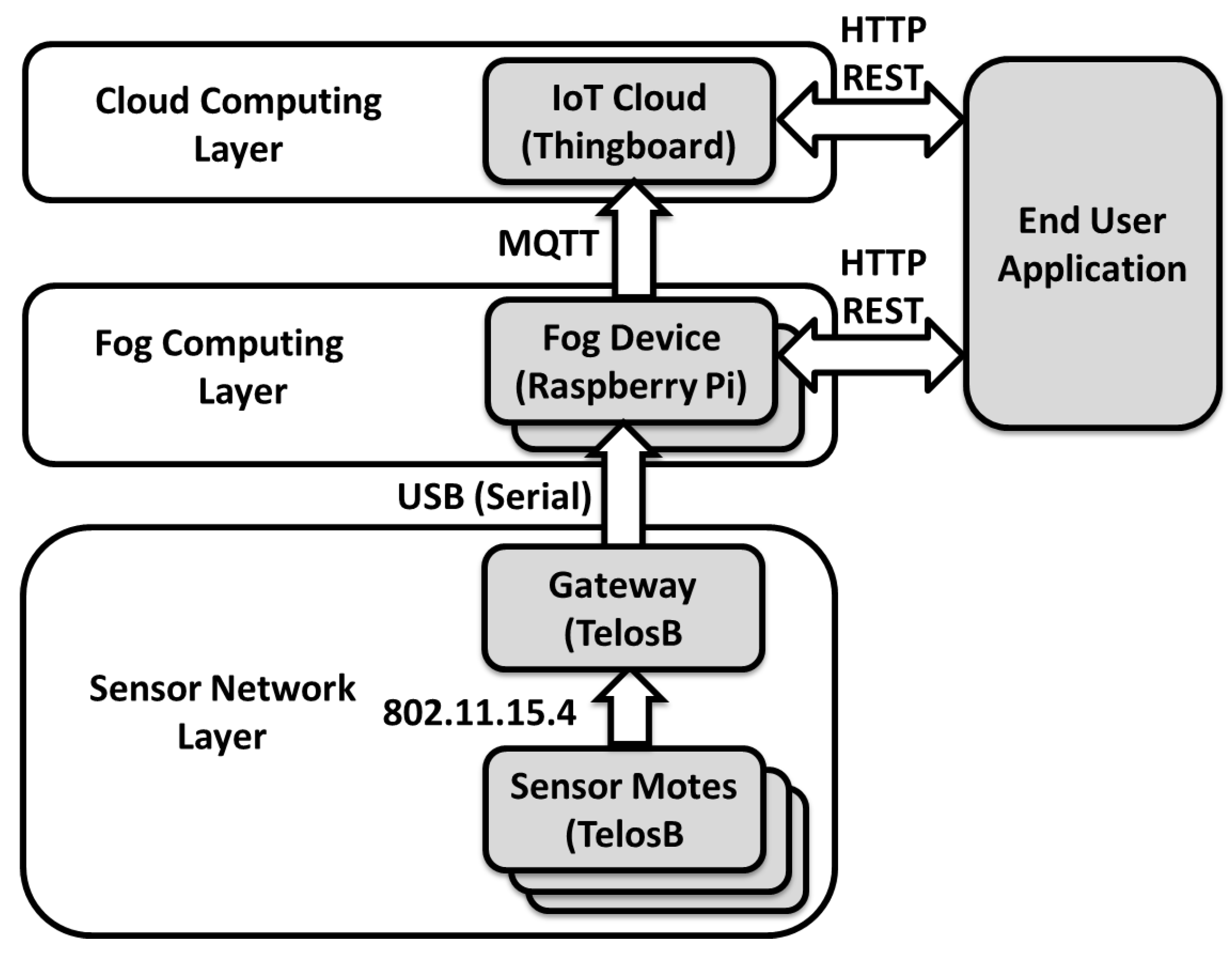
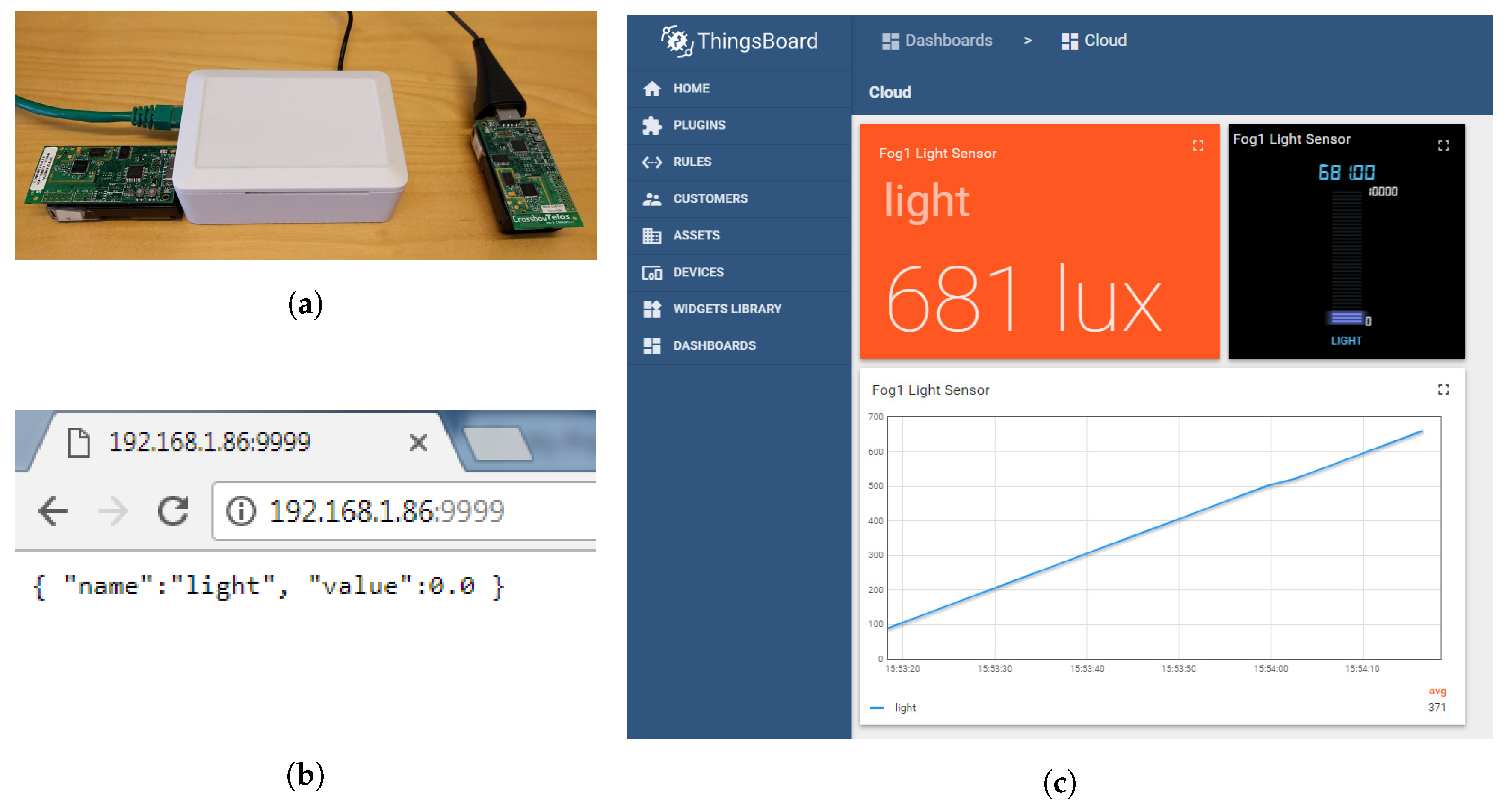
The proposed cloud, fog and sensor system works as expected. The sensor mote generates a sensor model from the raw sensor values, which is sent to the sensor gateway to reduce the required wireless communication. The fog system retrieves the model parameters from the sensor network layer, and regenerates the sensor values from the model parameters. The fog system both provides the sensor values directly to the end-user applications via a REST interface and sends the values to the cloud system via the MQTT protocol. On the cloud system, the values are persistently stored and the end user applications can access the sensor values in a more user-friendly manner.
Figure 7a shows the sensor motes and fog node with attached sensor gateway. A screenshot of the cloud dashboard with sensor values from the sensor motes via the model and fog device can be seen in
Figure 7c. The figure shows three different views of the same sensor value, as a card with exact value, as a digital gauge, and as an animated graph.
Figure 7b shows the output from the REST interface running on the fog devices. The output is a simple JSON object with the sensor name and its value.
As previously stated, the end-to-end delay was evaluated and measured in the testbed system. It was measured by adding together each of the steps in the proposed system. Firstly, from sensor node to end user application, secondly between the sensor mote to the fog node, thirdly between the fog node and the cloud node, and lastly between the cloud and end user application.
Each measurement was made 1000 times and the results of the evaluations can be seen in
Table 3, where
denotes the mean and
denotes the standard deviation of the measurements. Hence, we can see that the total delay is on average 180 ms with a standard deviation of 37 ms. It is, however, important to note that this is made in an optimal network situation where all devices are on the same network.
The query time of both the fog and cloud systems were also evaluated in the testbed. To measure query time we used the measurement laptop running a Java program that performs and measures the query response times of the respective REST interfaces on the fog and cloud. Results can be seen in
Table 4.
The experiments on the sensor layer, on both hardware implementation and Cooja simulation, show that the computational overhead has a negligible effect on delay with the chosen precision in the testbed, which is in the order of milliseconds, and the process still fits within the required sampling rate of 1 sample per second. The computational cost adds to processing time within the allocated time slot in magnitude of less than 2 ms. Finally, the scalability of the fog nodes was evaluated. Since we expect each fog device to handle multiple sensor motes and their models, we had to determine the maximum number of sensor values the fog device (Raspberry Pi) could handle from each sensor. According to measurement, the Raspberry Pi used on average 3.4 ms with a standard deviation of 1.8 ms for the serial communication to handle each sensor model update, which translates to about 290 sensor values per second. This means that each fog node can scale up to 290 sensor model updates per second. The realization of the proposed model in the form of the testbed system shows acceptable performance. Considering the presented results it is conceivable that the proposed model can meet the required latency of monitoring systems in industrial scenarios, as it can keep the performance above the required accuracy threshold.
6.3. Discussion
Considering the presented results, the distributed modeling at the WSN layer implemented on sensor devices, clearly reduces communication, hence saving spectrum. The simulation results of the fog layer clearly shows how approximations of the model parameter can regenerate the data stream at the fog node with acceptable accuracy. This is possible by providing the sensor nodes with transmission opportunities when detecting change points, instead of limiting them to a scheduled-based packet transmission. Furthermore, the prediction accuracy is enhanced by using more relevant statistical information about data streams. In addition to the presented results, an advantage of the proposed approach in comparison to other studies in this field, is that the model reduces some of the negative effects of wireless sensor communication on the performance of the learning algorithm, namely, synchronization of motes and high rate of dropped packets that adds additional delays to the learning process, and introduces the missing values problem to the learning algorithm.
It is worth mentioning that the presented model and testbed system are still under development. We consider the presented study a preliminary investigation of benefits of edge computing and its possible contribution to enhance network performance in IIoT. Moreover, we showed that it is possible to design cross-layer frameworks and to develop decentralized system models to implement collaborative systems by facilitating different communication standards. In the presented work, there are aspects that deserve more in-depth investigation. In the WSN layer, the complexity of the model can be reduced to make it more suitable for resource constraint devices. In addition, incorporating a more sophisticated medium access control protocol with prioritized packet handling mechanisms can be used to improve the reliability of the proposed model and expand its applicability over scenarios with various characteristics. Since the fog layer provides a localized view over the network, a fault detection mechanism can be deployed as a step toward decentralized fault detection and possible performance prediction. These are topics for future work.


