Multi-Target Angle Tracking Algorithm for Bistatic Multiple-Input Multiple-Output (MIMO) Radar Based on the Elements of the Covariance Matrix

National University of Defense Technology, Hefei 230037, China
*
Author to whom correspondence should be addressed.
Sensors 2018, 18(3), 805; https://doi.org/10.3390/s18030805
Submission received: 22 January 2018
/
Revised: 28 February 2018
/
Accepted: 1 March 2018
/
Published: 7 March 2018
(This article belongs to the Special Issue Sensor Signal and Information Processing)
Abstract
:In this paper, we consider the problem of tracking the direction of arrivals (DOA) and the direction of departure (DOD) of multiple targets for bistatic multiple-input multiple-output (MIMO) radar. A high-precision tracking algorithm for target angle is proposed. First, the linear relationship between the covariance matrix difference and the angle difference of the adjacent moment was obtained through three approximate relations. Then, the proposed algorithm obtained the relationship between the elements in the covariance matrix difference. On this basis, the performance of the algorithm was improved by averaging the covariance matrix element. Finally, the least square method was used to estimate the DOD and DOA. The algorithm realized the automatic correlation of the angle and provided better performance when compared with the adaptive asymmetric joint diagonalization (AAJD) algorithm. The simulation results demonstrated the effectiveness of the proposed algorithm. The algorithm provides the technical support for the practical application of MIMO radar.
1. Introduction
In recent years, the multiple-input multiple-output (MIMO) radar has been proposed as a new system radar [1]. Multiple array elements of the MIMO radar can transmit mutually orthogonal waveforms, which have a high degree of freedom [2,3,4]. Compared with the phased array radar, the MIMO radar has more accurate performance in target detection, identification, parameter estimation, and tracking. According to the array element configuration, the MIMO radar is divided into the statistical MIMO radar and coherent MIMO radar [5]. The array elements of the statistical MIMO radar are far away from each other, therefore, the statistical MIMO radar obtains spatial diversity gain, which can effectively improve the estimate performance of the scintillation target. The transmit and receive elements of the coherent MIMO radar are closely spaced, which can effectively improve the estimation accuracy of the target parameters, increase the number of the maximum identification targets, and so on. In the coherent MIMO radar, the bistatic MIMO radar is an important structure. The bistatic MIMO radar, which combines the advantages of MIMO radar and bistatic radar, effectively reduces the requirement of the three synchronizations (time, space, frequency). Therefore, the bistatic MIMO radar was used as the research object in this paper.
The existing parameter estimation algorithms in the bistatic MIMO radar are mostly aimed at stationary targets [6,7,8,9,10,11,12,13,14,15,16], which contain the estimation of signal parameters via rotational invariance technique (ESPRIT) algorithms [6,7,8,9], the Capon algorithm [10], the multiple signal classification (MUSIC) algorithms [11,12,13,14,15,16], and so on.
However, when the target is moving, the performance of the algorithm in [6,7,8,9,10,11,12,13,14,15,16] will decrease or even fail, which cannot be applied for tracking moving targets. The algorithms described above are all based on feature subspaces and require eigendecomposition. The computational complexity of the eigendecomposition process for the dimension square matrix is generally . The covariance matrix obtained in bistatic MIMO radar has a large dimension, which is the product of the number of transmitters and receivers. Therefore, the computational complexity required for eigendecomposition is large and the project realization is more difficult. In addition, these eigendecomposition and eigensubspace methods are a class of batch processing methods. Obviously, these algorithms cannot be applied to time-varying signals, but in the actual battlefield environment, the goal often moves. The target angle tracking is the key problem that restricts the practical application of bistatic MIMO radar. Therefore, this paper studies the angle tracking problem in bistatic MIMO radar.
There are some published studies on MIMO radar tracking. The monostatic MIMO radar tracking algorithm is given in [17], which has low complexity, but the cost is the reduction of tracking performance. In [18], Kalman was introduced into the projective approximation subspace tracking with deflation (PASTd) algorithm. The Kalman filter was used to realize data association, and the algorithm converges quickly. In [19], a low-complexity angle tracking algorithm in monostatic MIMO radar was proposed. The studies are all about target tracking for the monostatic MIMO radar.
Bistatic MIMO radar is different from monostatic MIMO radar and consists of a transmitting and receiving base. The corresponding direction of arrivals (DOA) and direction of departure (DOD) are not equal. Therefore, the joint steering vector is more complicated. The above algorithms in [17,18,19] cannot solve the problem of target tracking in bistatic MIMO radar.
In [20], the PASTd algorithm in the array-signal-processing was introduced to the bistatic MIMO radar, and the target tracking problem of the MIMO radar was successfully solved. However, it requires an additional data correlation operation and cannot track the targets of the same DOD or DOA. In order to solve the deficiency of [20], reference [21] proposed a low complexity tracking algorithm in bistatic MIMO radar. The algorithm deduces the formula of the covariance matrix difference of an adjacent moment, and then achieves the target angle tracking. However, the algorithm from [21] uses only partial covariance matrix information, and the tracking performance is low. A target tracking algorithm based on Adaptive Asymmetric Joint Diagonalization (AAJD) was proposed in [22]. The algorithm does not need an additional correlation operation and can track the targets whose DOD or DOA is the same. Nevertheless, the performance of the algorithm is reduced by reusing the estimation angle of the last time.
In this paper, we consulted the monostatic MIMO radar angle tracking idea in [19] to propose a DOD and DOA tracking algorithm suitable for bistatic MIMO radar. The covariance matrix, constructed by the monostatic MIMO radar signal, satisfied the Toeplitz form in [19]. However, the DOD and DOA were different and the covariance matrix did not satisfy the Toeplitz structure in the bistatic MIMO radar. Therefore, we proposed an improved DOA and DOD tracking method based on three approximations. Then, we found that the covariance matrix satisfied the approximate Toeplitz property, whose partial elements in a straight line paralleled to the principal diagonal were equal. On this basis, our algorithm used the approximate Toeplitz property to take the average operation, which was equivalent to improve the signal-to-noise ratio (SNR). The proposed algorithm could realize automatic matching and association of DOD and DOA. Error analysis was also derived in this paper. Finally, the simulation results were presented to verify the effectiveness of the proposed algorithm.
There were some differences between the algorithm in [19] and the proposed algorithm. (1) Reference [19] proposed a low-complexity angle tracking algorithm in monostatic MIMO radar. However, we solved the DOD and DOA tracking problems of the bistatic MIMO radar. (2) The monostatic MIMO radar only needed to estimate DOA, but the algorithm in this paper needed to solve the DOD and DOA estimation, therefore the problem is more complicated. In this paper, the algorithm extended the approximate idea in [19] and solved the target angle by three approximation operations. (3) The monostatic MIMO radar angle tracking algorithm requires that the covariance matrix satisfy the Toeplitz form. Since the DOD and DOA are different, the covariance matrix is more complicated and does not satisfy the Toeplitz form in bistatic MIMO radar. Therefore, the algorithm in [19] cannot be used to solve the problem directly in this paper. So we used the approximate Toeplitz properties to improve the tracking performance.
Thus, the algorithm cannot only be seen as an extension of the work in [19] but is also an improved algorithm. The simulation results showed that the proposed algorithm had a better tracking performance than the angle tracking algorithm in [19,20,21,22].
The rest of this paper is organized as follows. In Section 2, the signal model of bistatic MIMO radar is presented. Section 3 establishes our angle tracking algorithm based on the elements of the covariance matrix of the receive signal. Section 4 compares the performance of the algorithm in [19,20,21,22] and our algorithm. The simulation results verify the effectiveness of the proposed algorithm. Finally, Section 5 concludes the paper.
Notations: , , , and denote the transpose, Hermitian transpose, pseudoinverse and inverse operations, respectively. is an identity matrix; is the vectorization of a matrix; stands for diagonal matrix whose diagonal is a vector ; and are the Kronecker product and Hadamard product, respectively.
2. Signal Model
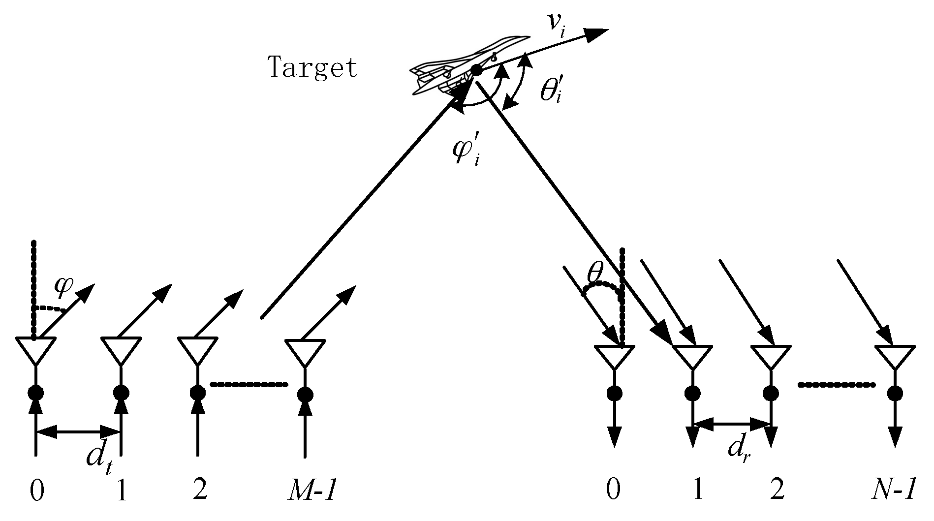
In this paper, a bistatic MIMO radar was used to observe the moving targets in the air. The distances between the targets and bases are far, so the target satisfies the point target model. The bistatic MIMO radar is composed of transmit antennas and receive antennas. The space between the transceiver antennas is the same and half of the wavelength. The configuration of the bistatic MIMO radar is shown in Figure 1.
It is assumed that there is a far-field moving point target in the air, and the DOD and DOA at time is , respectively. The velocity of the target is , and the angles between the moving direction and the DOD and DOA directions are and , respectively.
The transmit signal radiates to targets, and the signal that arrives at the receive elements after scattering is
where ; is the doppler shift. The receive steering vector is ; and the transmit steering vector is . is the scattering coefficient of the observation target and satisfies the Swerling II model, which is invariable within the pulse time. , is Gaussian additive white noise.
The signal is filtered through a set of matched filters, let each filter match only one transmit signal. Let the delay of matched filter of th target signal is , and .
The output of the signal in Equation (2) after matched filtering is
and has the same statistical properties, still satisfy the Swerling II model. The mean and variance of is and .
Further simplify Equation (3),
Consider the vectorization of in (4),
where denotes joint steering vector.
Consider
where , .
Assuming that DOD and DOA change slowly, and consider that the DOD and DOA of the target are the same in the time interval , and are uncorrelated for the different targets and all targets are in the same range bin. During the interval , remains constant and snapshots of sensor data are available for the signal processing.
3. Angle Tracking Algorithm Description
The angle tracking algorithm in [19] requires that the steering vector satisfies the Vandermonde form. The joint steering vector in Equation (4) does not satisfy the Vandermonde form, so the angle tracking algorithm in [19] cannot be applied directly to bistatic MIMO radar. We improved the algorithm in [19] and proposed an angle tracking algorithm suitable for bistatic MIMO radar.
3.1. Estimation of the Covariance Matrix Difference and the Angle Difference
At the time , the DOD and DOA of the targets are recorded as . Similarly, the DOD and DOA at time is recorded as .
We define
where is the angle difference between and , and .
We define as the covariance matrices of the signal at time . The covariance matrices are
then we can obtain
Supposing that the noise covariance matrix at time is approximately equal to that at time , then we have
It can be seen that the covariance matrix difference of adjacent moment is caused by the angle difference of adjacent moment, so there is a relationship between the two. Therefore, by deriving the relationship between the two, the angle difference of adjacent moment can be obtained.
3.2. Estimation of DOD and DOA
In Section 3.1, we obtained the covariance matrix difference and the angle difference . This section will deduce the linear relationship between the covariance matrix difference and the angle difference.
We first analyzed the properties of the elements of the covariance matrix. The literature [19] proved that in Equation (9) can be expressed as
where , .
where is the element of the matrix and , . in Equation (11) can be expanded as
From Equation(12), it can be see that is related to the angle difference and the angle of the previous moment. and are the parameters to be estimated. Considering that and is very small,
substituting Equations (13) and (14) into Equation(12), then in Equation (12) can be denoted as
Considering that is very small, . Then, can be rewritten as
By Equation(16), we can construct the following equation
where
To give the , we define , , , .
Using the least square method to estimate in Equation (17), we get
The final estimate of the angle is
3.3. Covariance Element Average Operation
The algorithm in [19] makes full use of the Toeplitz matrix property to improve performance. Since the joint steering vector of bistatic MIMO radar does not satisfy the Vandermonde form, the covariance matrix difference does not satisfy the Toeplitz property. Therefore, we first analyzed the structure of the steering vector.
It can be found that some elements in the steering vector satisfied the Vandermonde structure in Equation (23). This structure is called the approximate Vandermonde structure in this paper.
We further analyzed the structure of the covariance matrix, taking as an example.
Since the steering vector satisfied the approximate Vandermonde structure, the sub-matrices in a straight line parallel to the principal diagonal of are the same. has a similar structure.
From the above analysis, we can see that is an approximate Toeplitz matrix whose sub-matrices in a straight line parallel to the principal diagonal are the same. We used the average operation to estimate and to eliminate the noise. The following steps can be used to update the and .
where is the element of the matrix . Substituting Equation (25) into Equation (18), then can be rewritten as
The proposed algorithm fully uses the approximate Toeplitz matrix property and more receiving information to eliminate the noise, and improve angle tracking performance. Now, we discuss the performance comparison between our algorithm and the algorithms in the literature [19,20,21,22].
The AAJD and PASTd algorithm sestimate the target angle through optimizing the function. Because it is difficult to find the optimal solution of the optimization function, the performance of the algorithm is low. The algorithm in [19,21] and our algorithm obtain angle via the difference between the previous and current covariance matrix of the receiving signal. So the performance of the algorithm in [19,21] and our algorithm is better than the AAJD and PASTd algorithms.
The algorithm in [19] can be improved to solve the angle tracking problem of bistatic MIMO radar, but it only uses the elements of the covariance matrix ( is the number of transmit antennas, and is the number of receive antennas). The algorithm in [21] and our algorithm uses the and elements of the covariance matrix to track the target, respectively. Owning to , the proposed algorithm used more covariance matrix information than the algorithm in [19,21]. So, the performance of our algorithm was better than that of [19,21].
In summary, the performance of our algorithm was the best.
Until now, we show the major steps of the angle tracking algorithm in bistatic MIMO radar as follows.
Step 1. Calculate the covariance matrix and via Equations (5) and (7).
Step 2. Calculate the covariance matrix difference via Equation (10).
Step 3. The vector is obtained via Equation (26), and the vector is obtained via Equation (20).
Step 4. We estimate via Equation (21), and the angle at time is .
Step 5. Repeat steps 1 to 4 to estimate the angle of the next moment.
- Note 1.
- This paper assumes that the number of targets in the bistatic MIMO radar is known. If we do not know the number in advance, we can use the existing target-number estimation algorithm in [23] to estimate the number of targets.
- Note 2.
- The algorithm in this paper only obtains the angle difference of adjacent time, and therefore we need to get the initial DOD and DOA of the target. The initial DOD and DOA can be obtained using the MUSIC algorithm or another angle estimation algorithm.
- Note 3.
- The algorithm in this paper was valid effectively when the target velocity was low and the DOD and DOA changed slowly. When the target moves faster, the performance of the algorithm in this paper will be reduced or even invalidated. When the target was far from the transceiver base, the angle difference was generally small, so this algorithm is suitable for tracking the long-distance target.
- Note 4.
- The noise covariance matrices of adjacent time can be approximately assumed to be equal. No matter what kind of noise, the noise component in Equation (8) can be eliminated. The algorithm is still effective under the colored noise conditions.
3.4. Computational Complexity Analysis and Advantages of the Proposed Algorithm
For the proposed algorithm, the calculation of the covariance matrix needs , and the computation of requires . The main computational complexity of the proposed algorithm is .
The advantages of this algorithm are listed as follows:
- (1)
- The proposed algorithm does not need eigenvalue decomposition of the covariance matrix, so the complexity is lower.
- (2)
- The proposed algorithm not only introduces the tracking algorithm in [19], but also expands it.
- (3)
- The proposed algorithm makes full use of the elements in the covariance matrix to improve the tracking performance. The performance of this algorithm is better than the AAJD algorithm.
- (4)
- The algorithm in this paper can automatically match and associate the angles of adjacent moment and reduce the computational complexity.
4. Error Analysis
In this section, we deduce the variance of DOD and DOA tracking. We assume that the observed noise variances are nearly the same at the adjacent time. When estimating DOD and DOA, we used approximate calculations such as and when was smaller. This leads to a slight difference from the real value. Consider
where , , and are the high-order expansion terms.
According to Equations (13), (14), (27) and (28), we have
By Equations (15), (16), and (29), then
is the estimation error of , and can be shown as follows:
According to Equations (21) and (32), the variance of is denoted by
Then, we have
We define that is the estimation error of .
Then the variance of is
According to [24], we get the variance of
where denotes the th row of and is the pseudoinverse of . According to Equations (33)–(35) and (37), we get
where is shown in Equation (37).
From Equations (37) and (39), we can obtain an effective conclusion where the theoretical variance of the proposed algorithm is gradually decreased with the number of transmit/receive antennas increases. Multiple transmit/receive antennas improve the angle tracking performance.
5. Simulation Results
Assuming that both the transmit and receive arrays of the bistatic MIMO radar are linearly configured, the spacing of the array elements is half wavelength. The carrier frequency of the array element is , the pulse width is , and the pulse repetition rate is . The emission waveform uses the Hadamard Code Pulse (HCP) signal, and the number of the transmit and receive array elements is (except experiments 6,7). We defined the root-mean square error (RMSE) as , where and is the estimate of angle and ; are the times of the Monte Carlo trial. The targets are tracked over an interval of s, during each s interval, snapshots of sensor data are generated and used to estimate angles.
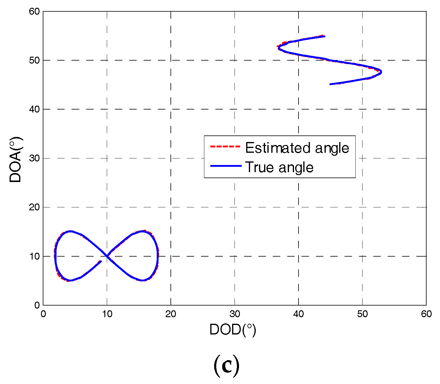
Figure 2 shows the result of the tracking angle of the targets of uniform speed for , , and . The simulation results showed that the estimated trajectory coincided with the real trajectory, which proved the effectiveness of the algorithm.
Figure 3 depicts the tracking result of the proposed algorithm for non-uniform moving targets and showed that our algorithm could successfully track the moving target at a non-uniform speed. The DOD and DOA could be automatically associated. The estimated angle trajectory coincided with the true trajectory, indicating the effectiveness and robustness of the proposed algorithm.
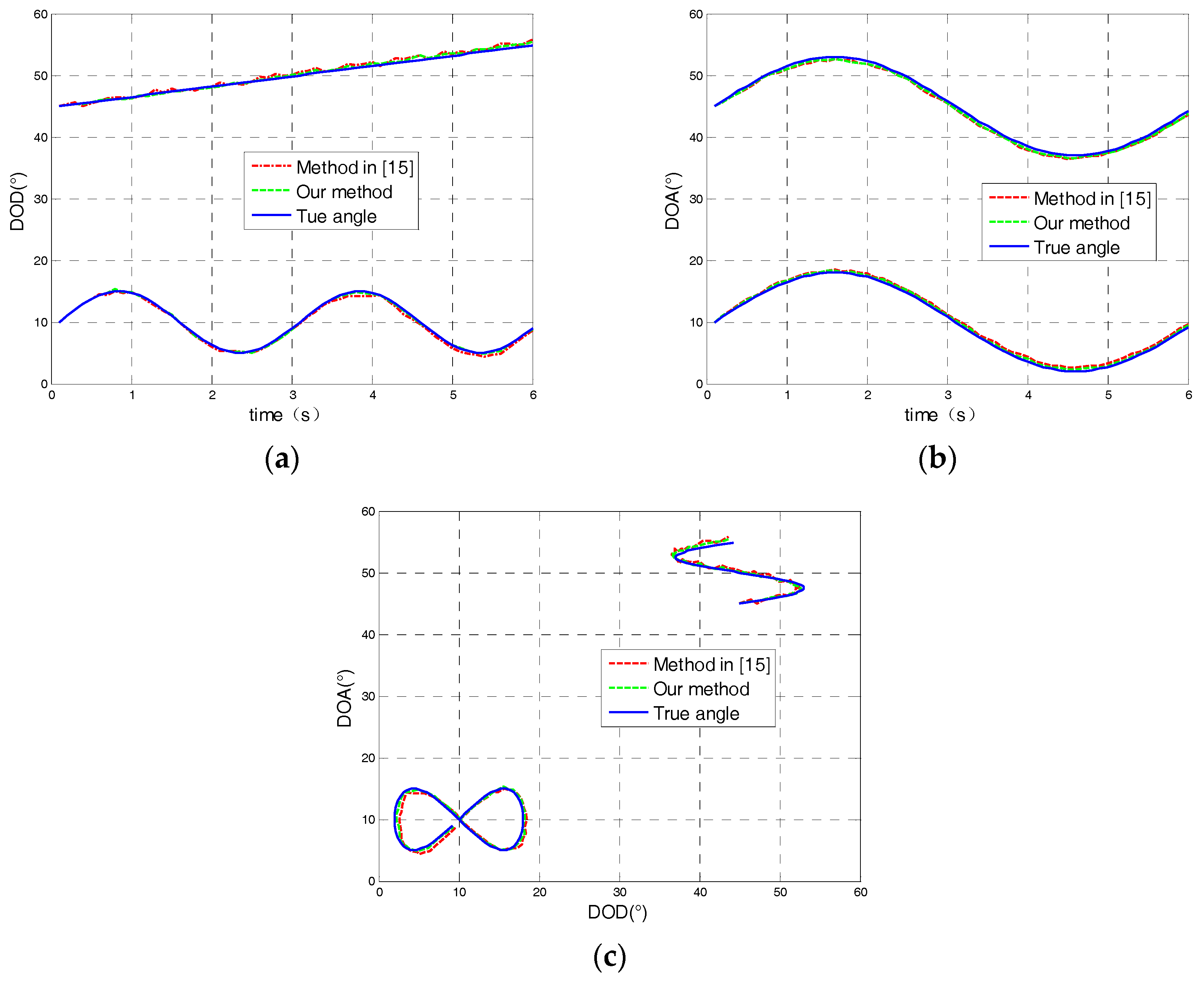
Figure 4 depicts the tracking result comparison between the proposed algorithm and the angle tracking algorithm in [19] with . From Figure 4, it can be seen that the tracking result of our algorithm had a high degree of coincidence with the real trajectory of the target, and the performance was better than the tracking algorithm in [19].
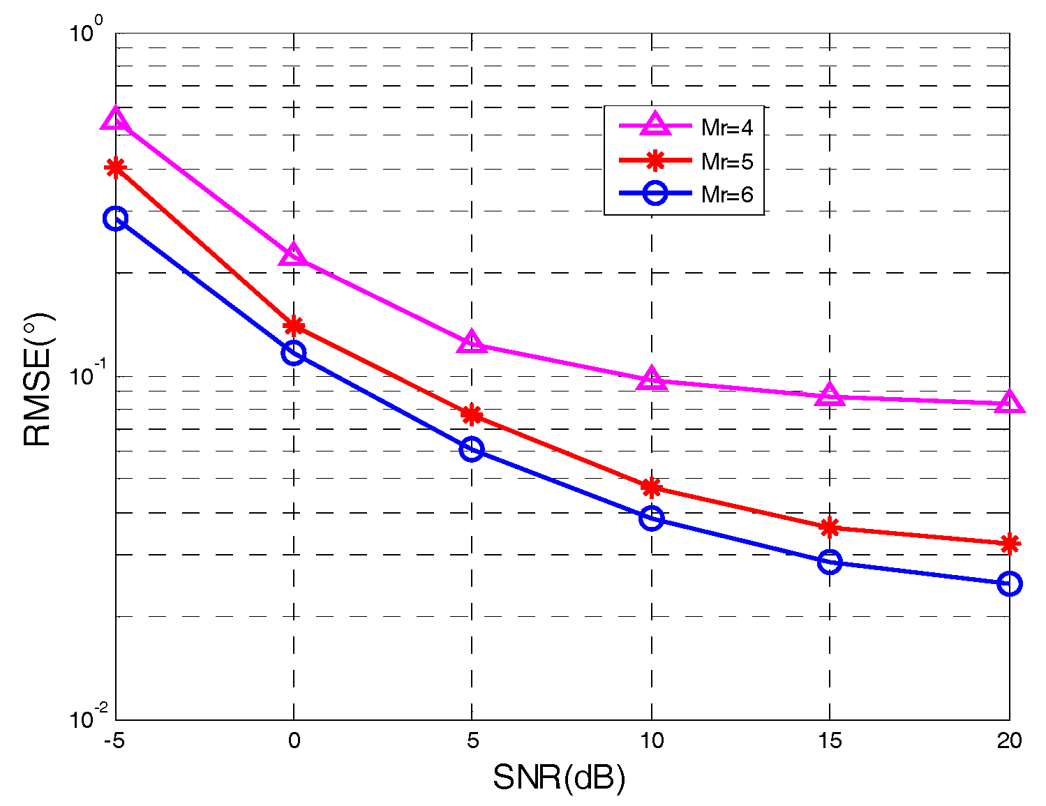
To better verify the performance of the proposed algorithm, Figure 5 shows the tracking performance comparison with , , , and , where we compared the proposed algorithm against the angle tracking algorithm in [19,21], the PASTd algorithm in [20], and AAJD algorithm in [22]. At the same time, we gave the theoretical error caused by the approximate operation. It can be seen from Figure 5 that the RMSE of our algorithm was lower than that of the angle tracking algorithm in [19,21], PASTd algorithm, and AAJD algorithm, which showed that the tracking performance of our algorithm was the best and the correctness of the theoretical analysis was verified. This was because the proposed algorithm made full use of the elements of covariance matrix to eliminate the noise and improved the estimation performance. The theoretical variance was lower than the actual variance, because the noise was ignored when the theoretical variance is derived.
Figure 6 and Figure 7 display the performance of angle tracking via our algorithm in the condition of , , , , and variable numbers of . It was clearly shown that the angle tracking performance of the proposed algorithm gradually improved with the increased number of transmit/receive antennas. Multiple transmit/receive antennas improved the angle tracking performance because of diversity gain. The correctness of the conclusions drawn from the theoretical error was validated.
6. Conclusions
In this paper, we proposed a moving multi-target angle tracking algorithm for bistatic MIMO radar. The proposed algorithm obtained the linear relationship between the covariance matrix difference and the angle difference through the three approximate processes. The proposed algorithm reduced the computational complexity and realized the automatic association of DOA and DOD. The proposed algorithm made full use of the elements of the covariance matrix by taking the average method, eliminating the noise, and improving the tracking performance. The research in this paper provides technical support for the practical application of the MIMO radar. In future work, we will analyze wideband signal processing to improve performance [25,26] and study signal processing in complex backgrounds to increase the robustness of the algorithm.
Author Contributions
Zhengyan Zhang and Jianyun Zhang participated in the design of this study. Zhengyan Zhang and Qingsong Zhou conceived and designed the experiments and performed the experiments; Zhengyan Zhang and Xiaobo Li analyzed the result of the experiments; Zhengyan Zhang wrote the paper.
Conflicts of Interest
The authors declare no conflict of interest.
References
- Fishler, E.; Haimovich, A.; Blum, R.; Chizhik, D.; Cimini, L.; Valenzuela, R. MIMO radar: An idea whose timehas come. In Proceedings of the IEEE Radar Conference, Philadelphia, PA, USA, 26–29 April 2004; pp. 71–78. [Google Scholar]
- Li, J.; Stoica, P. MIMO Radar with Colocated Antennas. IEEE Signal Process. Mag. 2007, 24, 106–114. [Google Scholar] [CrossRef]
- Haimovich, A.M.; Blum, R.S.; Cimini, L.J. MIMO Radar with Widely Separated Antennas. IEEE Signal Process. Mag. 2008, 25, 116–129. [Google Scholar] [CrossRef]
- Wang, X.P.; Huang, M.X.; Wu, X.Q.; Bi, G.A. Direction of arrival estimation for MIMO radar via unitary nuclear norm minimization. Sensor 2017, 17, 939. [Google Scholar] [CrossRef] [PubMed]
- Tang, B.; Tang, J. Joint Design of Transmit Waveforms and Receive Filters for MIMO Radar Space-Time Adaptive Processing. IEEE Trans. Signal Process. 2016, 64, 4707–4722. [Google Scholar] [CrossRef]
- Zheng, G.M.; Tang, J.; Yang, X. ESPRIT and Unitary ESPRIT Algorithms for Coexistence of Circular and Noncircular Signals in Bistatic MIMO Radar. IEEE Access 2016, 4, 7232–7240. [Google Scholar] [CrossRef]
- Wang, W.; Wang, X.; Song, H.; Ma, Y. Conjugate ESPRIT for DOA estimation in monostatic MIMO radar. Signal Process. 2013, 93, 2070–2075. [Google Scholar] [CrossRef]
- Yang, X.; Zheng, G.M.; Tang, J. ESPRIT algorithm for coexistence of circular and noncircular signals in bistatic MIMO radar. In Proceedings of the 2016 IEEE Radar Conference (RadarConf), Philadelphia, PA, USA, 2–6 May 2016; pp. 1–4. [Google Scholar]
- Li, J.F.; Jiang, D.F.; Zhang, X.F. DOA estimation based on combined unitary ESPRIT for coprime MIMO radar. IEEE Commun. Lett. 2017, 21, 96–99. [Google Scholar] [CrossRef]
- Zhang, X.; Huang, Y.; Chen, C.; Li, J.; Xu, D. Reduced complexity Capon for direction of arrival estimation in a monostatic multiple-input multiple-output radar. IET Radar Sonar Navig. 2012, 6, 796–801. [Google Scholar] [CrossRef]
- Belfiori, F.; Rossum, W.V.; Hoogeboom, P. Coherent MUSIC technique for range/angle information retrieval: Application to a frequency-modulated continuous wave MIMO radar. IET Radar Sonar Navig. 2014, 8, 75–83. [Google Scholar] [CrossRef]
- Tan, J.; Nie, Z.P.; Wen, D.B. Low complexity MUSIC-based direction-of-arrival for monostatic MIMO radar. Electron. Lett. 2017, 53, 275–277. [Google Scholar] [CrossRef]
- Zahernia, A.; Dehahani, M.J.; Javidan, R. MUSIC algorithm for DOA estimation using MIMO arrays. In Proceedings of the 2011 Sixth International Conference on Telecommunication Systems, Services, and Application, Bali, Indonesia, 20–21 October 2011; pp. 149–153. [Google Scholar]
- Devaney, A.J. Time reversal imaging of obscured targets from multistatic data. IEEE Trans. Antennas Propag. 2005, 53, 1600–1610. [Google Scholar] [CrossRef]
- Ciuonzo, D.; Romano, G.; Solimene, R. Performance analysis of time-reversal MUSIC. IEEE Trans. Signal Process. 2015, 63, 2650–2662. [Google Scholar] [CrossRef]
- Ciuonzo, D.; Salvo, R.P. Noncolocated time-reversal MUSIC: High-SNR distribution of null spectrum. IEEE Signal Process. Lett. 2017, 24, 397–401. [Google Scholar] [CrossRef]
- Wu, H.L.; Zhang, X.F. DOA tracking in monostatic MIMO radar using PARAFAC-RLST algorithm. In Proceedings of the 3rd International Conference on Information Science and Engineering (ICISE’11), Yangzhou, China, 29 September–1 October 2011; pp. 958–961. [Google Scholar]
- Zhang, X.F.; Li, J.F.; Feng, G.P.; Wu, H.L. Kalman-PASTd based DOA tracking algorithm for monostatic MIMO radar. In Proceedings of the International Conference on Information, Services and Management Engineering, Beijing, China, 26–28 December 2011; pp. 220–224. [Google Scholar]
- Yu, H.X.; Zhang, X.F.; Chen, X.Q.; Wu, H.L. Computationally efficient DOA tracking algorithm in monostatic MIMO radar with automatic association. Int. J. Antennas Propag. 2014, 2014. [Google Scholar] [CrossRef]
- Wu, H.; Zhang, X. DOD and DOA tracking algorithm for bistatic MIMO radar using PASTD without additional angles pairing. In Proceedings of the IEEE 5th International Conference on Advanced Computational Intelligence (ICACI’12), Nanjing, China, 18–20 October 2012; pp. 1132–1136. [Google Scholar]
- Zhang, Z.Y.; Li, X.B.; Xu, X.Y.; Huang, C. Target angle rapid tracking algorithm for bistatic MIMO radar. J. Signal Process. 2016, 32, 701–706. (In Chinese) [Google Scholar]
- Zhang, W.T.; Lou, S.T.; Li, X.J. Tracking multiple target in MIMO radar Via adaptive asymmetric joint diagonalization. IEEE Trans. Signal Process. 2016, 64, 2880–2893. [Google Scholar] [CrossRef]
- Xin, J.M.; Zheng, N.N.; Sano, A. Simple and efficient nonparametric method for estimating the number of signals without eigendecomposition. IEEE Trans. Signal Process. 2007, 55, 1405–1420. [Google Scholar] [CrossRef]
- Rao, B.D.; Hari, K.V.S. Performance analysis of ESPRIT and TAM in determining the direction of arrival of plane waves in noise. IEEE Trans. Acoust. Speech Signal Process. 1989, 37, 1990–1995. [Google Scholar] [CrossRef]
- Shi, G.; Nehorai, A. Maximum Likelihood Estimation of Point Scatterers for Computational Time-reversal Imaging. Commun. Inf. Syst. 2005, 5, 227–256. [Google Scholar]
- Ciuonzo, D. On Time-Reversal Imaging by Statistical Testing. IEEE Signal Process. Lett. 2017, 24, 1024–1028. [Google Scholar] [CrossRef]
Figure 1.
Bistatic multiple-input multiple-output (MIMO) radar transceiver element configuration.

Figure 2.
Angle tracking results of uniform moving target at : (a) The direction of departure (DOD); (b) The direction of arrival (DOA); (c) DOD and DOA trajectory.
Figure 2.
Angle tracking results of uniform moving target at : (a) The direction of departure (DOD); (b) The direction of arrival (DOA); (c) DOD and DOA trajectory.
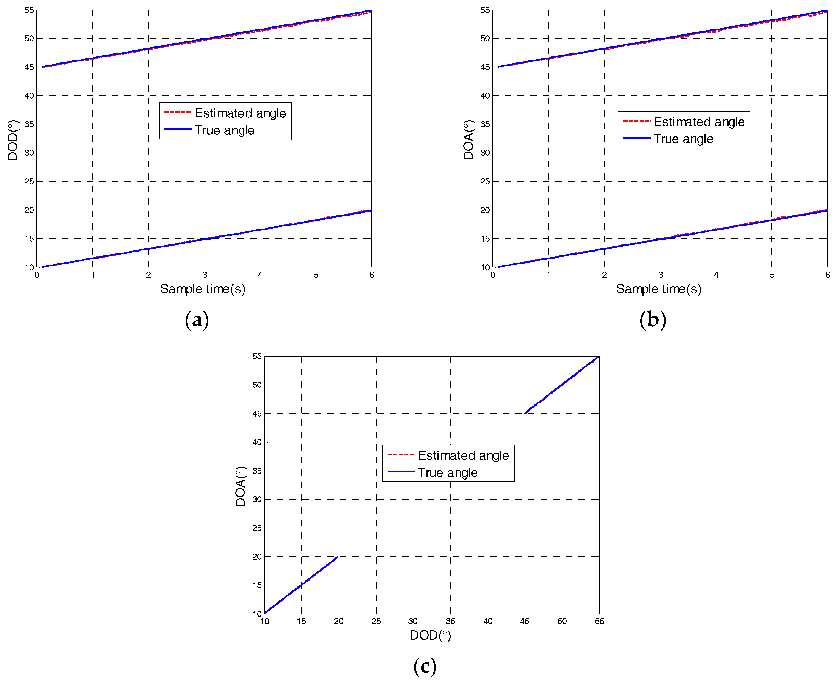
Figure 3.
Angle tracking results of non-uniform moving targets with : (a) The direction of departure; (b) The direction of arrival; (c) DOD and DOA trajectory.
Figure 3.
Angle tracking results of non-uniform moving targets with : (a) The direction of departure; (b) The direction of arrival; (c) DOD and DOA trajectory.
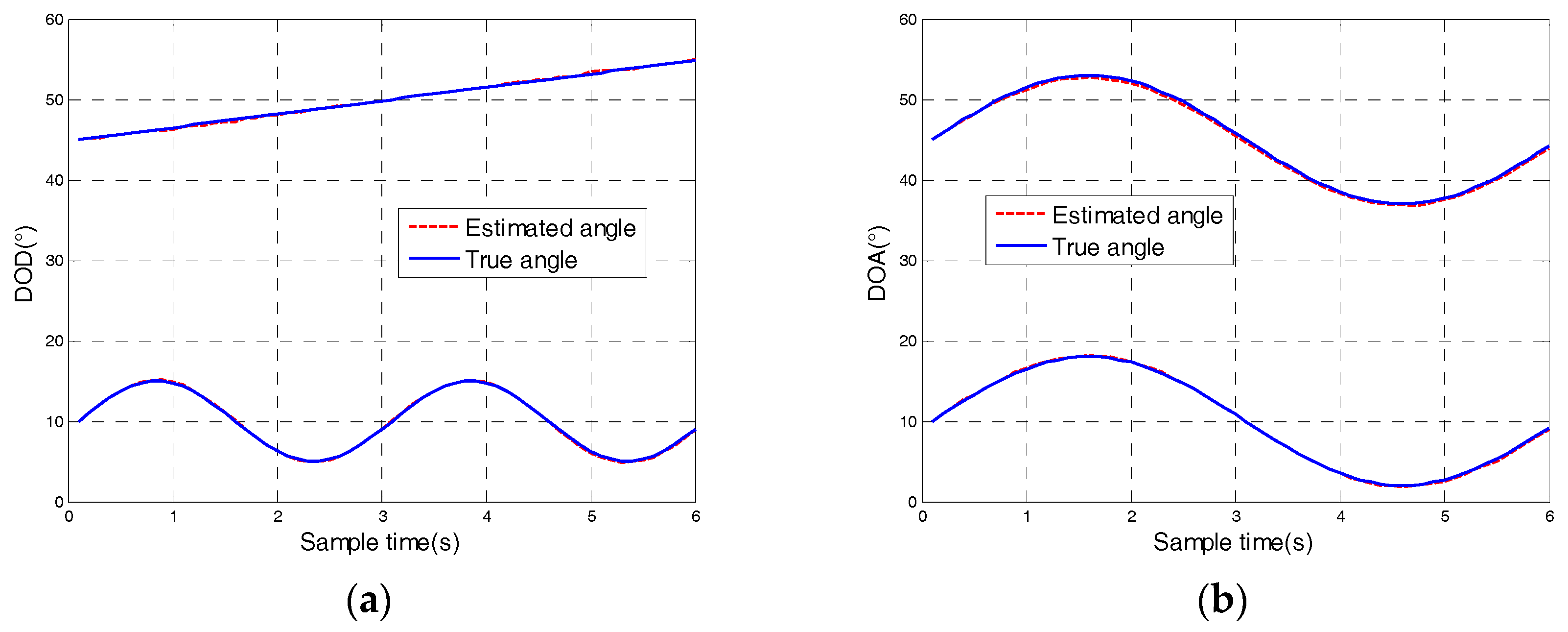

Figure 4.
Angle tracking result comparison with : (a) The direction of departure; (b) The direction of arrival; (c) DOD and DOA trajectory comparison.
Figure 4.
Angle tracking result comparison with : (a) The direction of departure; (b) The direction of arrival; (c) DOD and DOA trajectory comparison.

Figure 5.
RMSE changes with signal-to-noise ratio (SNR).
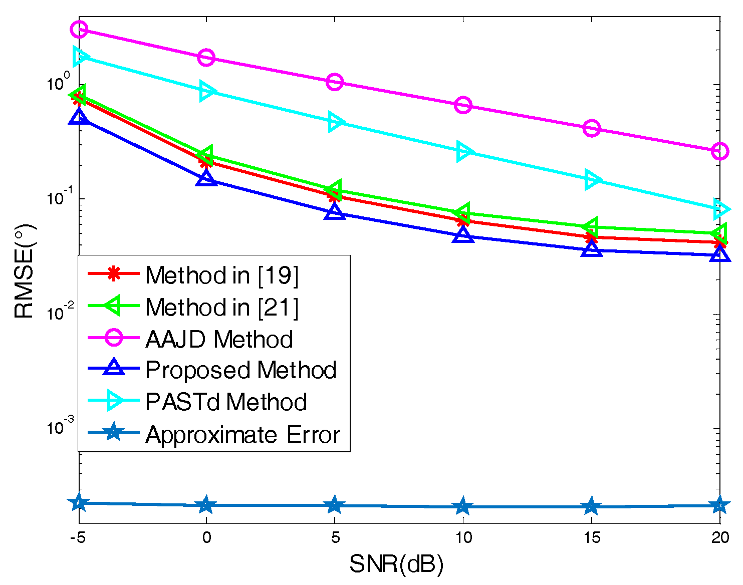
Figure 6.
Angle tracking with different values of .
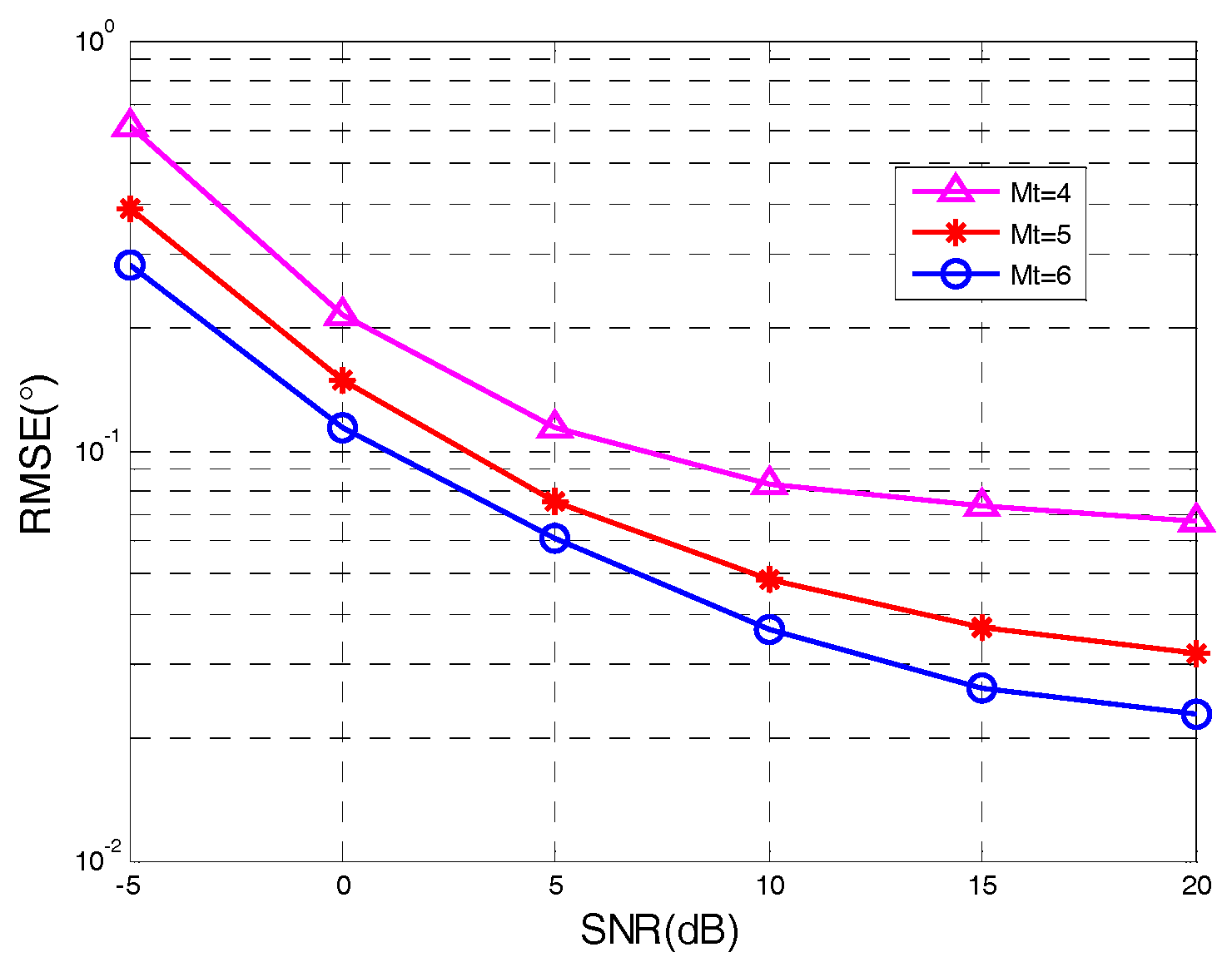
Figure 7.
Angle tracking with different values of .

© 2018 by the authors. Licensee MDPI, Basel, Switzerland. This article is an open access article distributed under the terms and conditions of the Creative Commons Attribution (CC BY) license (http://creativecommons.org/licenses/by/4.0/).
Share and Cite
MDPI and ACS Style
Zhang, Z.; Zhang, J.; Zhou, Q.; Li, X. Multi-Target Angle Tracking Algorithm for Bistatic Multiple-Input Multiple-Output (MIMO) Radar Based on the Elements of the Covariance Matrix. Sensors 2018, 18, 805. https://doi.org/10.3390/s18030805
AMA Style
Zhang Z, Zhang J, Zhou Q, Li X. Multi-Target Angle Tracking Algorithm for Bistatic Multiple-Input Multiple-Output (MIMO) Radar Based on the Elements of the Covariance Matrix. Sensors. 2018; 18(3):805. https://doi.org/10.3390/s18030805
Chicago/Turabian StyleZhang, Zhengyan, Jianyun Zhang, Qingsong Zhou, and Xiaobo Li. 2018. "Multi-Target Angle Tracking Algorithm for Bistatic Multiple-Input Multiple-Output (MIMO) Radar Based on the Elements of the Covariance Matrix" Sensors 18, no. 3: 805. https://doi.org/10.3390/s18030805
Note that from the first issue of 2016, this journal uses article numbers instead of page numbers. See further details here.