Comparison of Different Algorithms for Calculating Velocity and Stride Length in Running Using Inertial Measurement Units


Abstract
:1. Introduction
1.1. Literature Review
1.2. Contribution
2. Methods
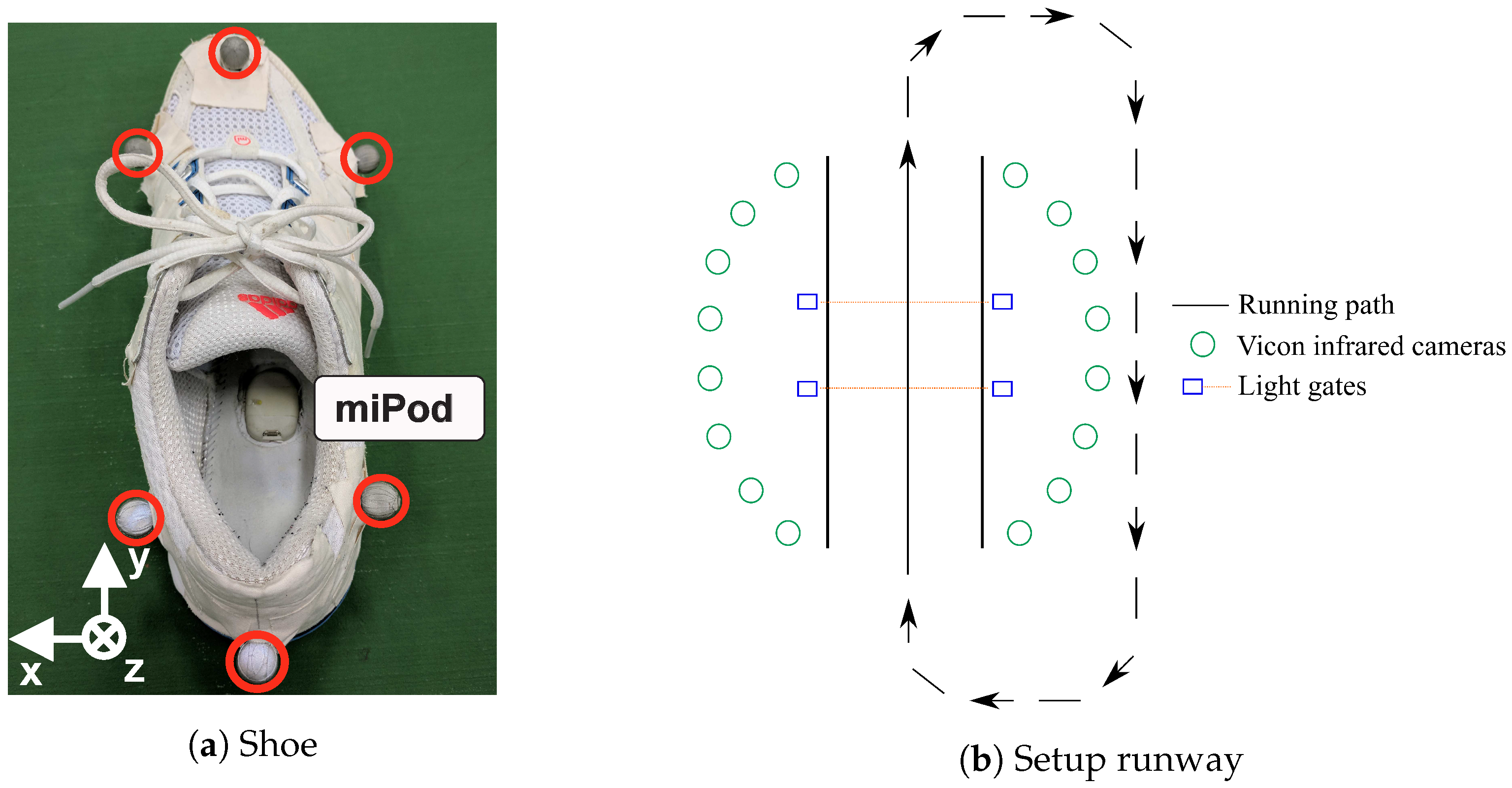
2.1. Data Collection
2.1.1. Lab Study
2.1.2. Field Study
2.2. Algorithms
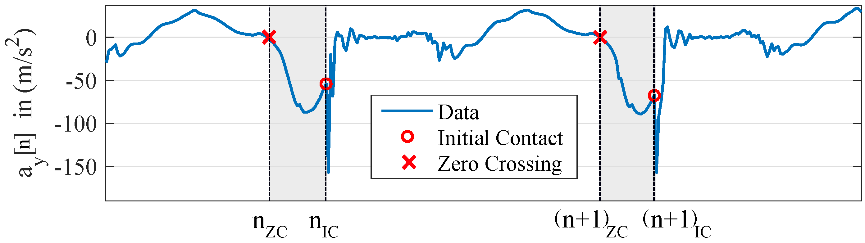
2.2.1. Stride Segmentation
2.2.2. Stride Time
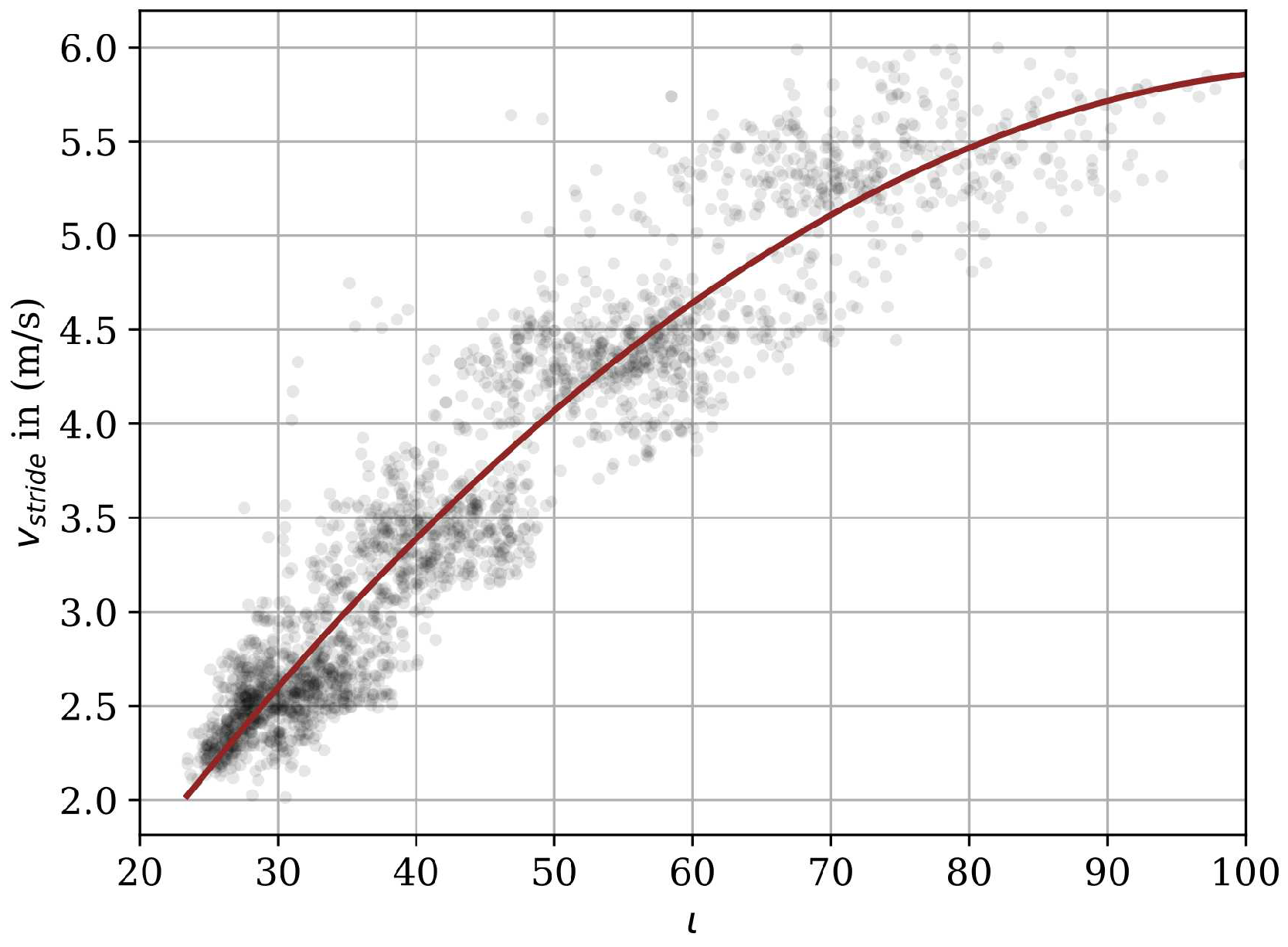
2.2.3. Acceleration
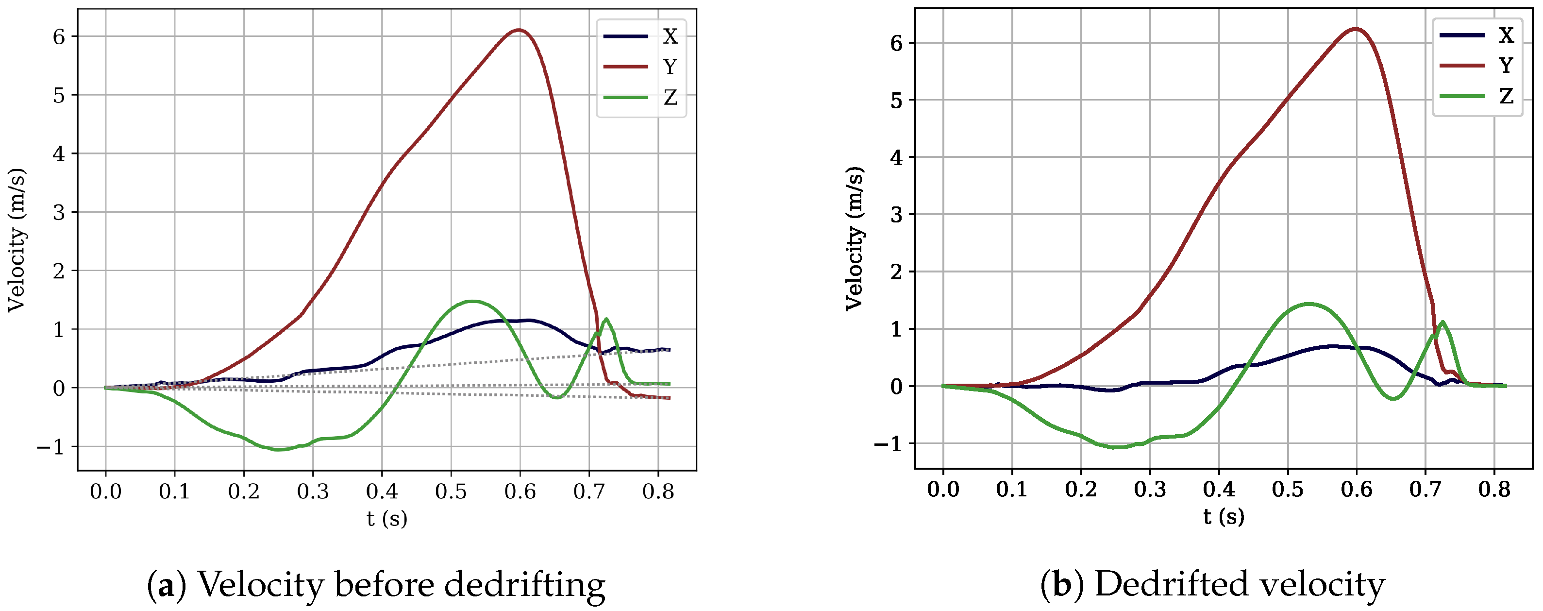
2.2.4. Trajectory
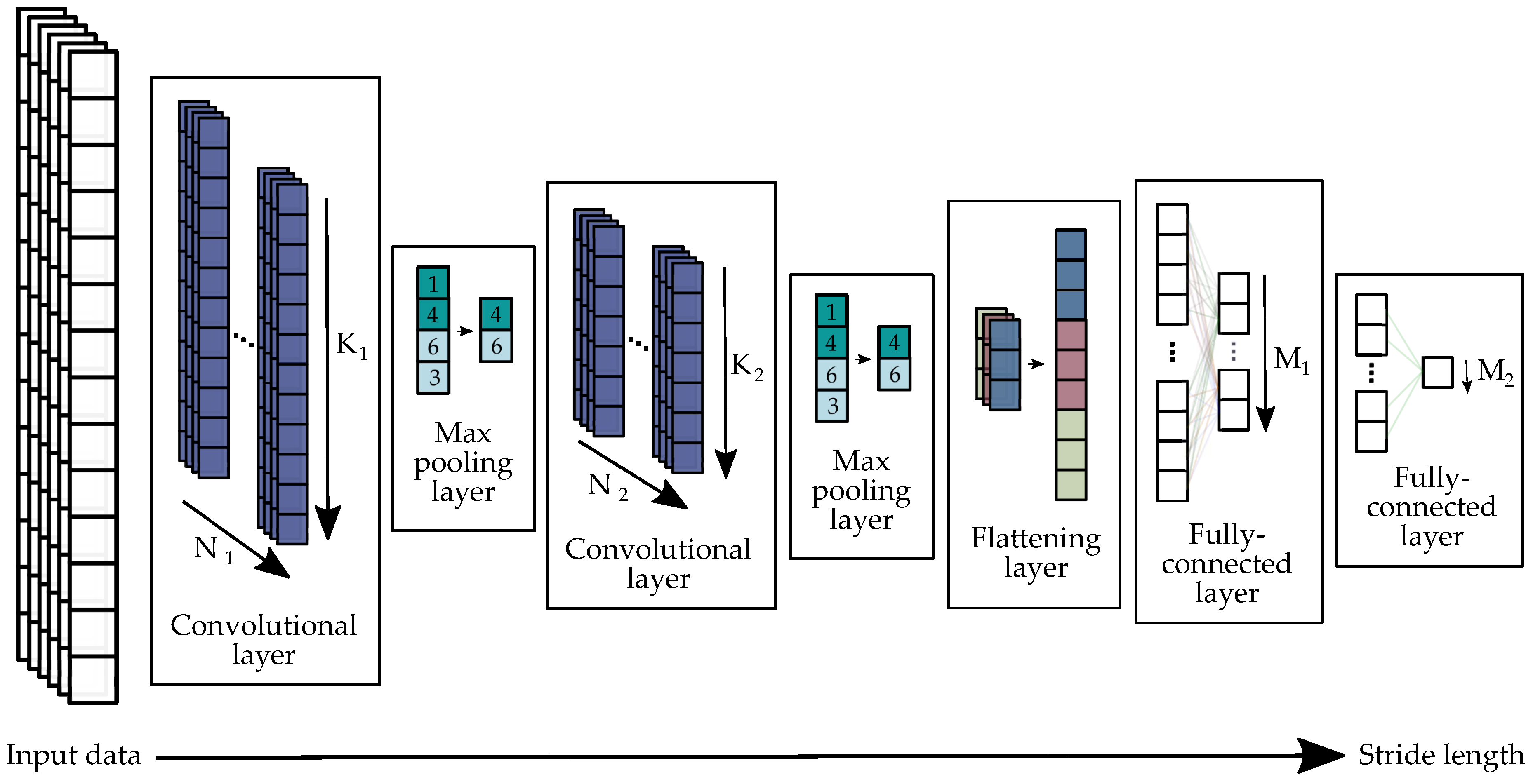
2.2.5. Deep Learning
2.3. Evaluation
2.3.1. Lab Study
2.3.2. Field Study
3. Results
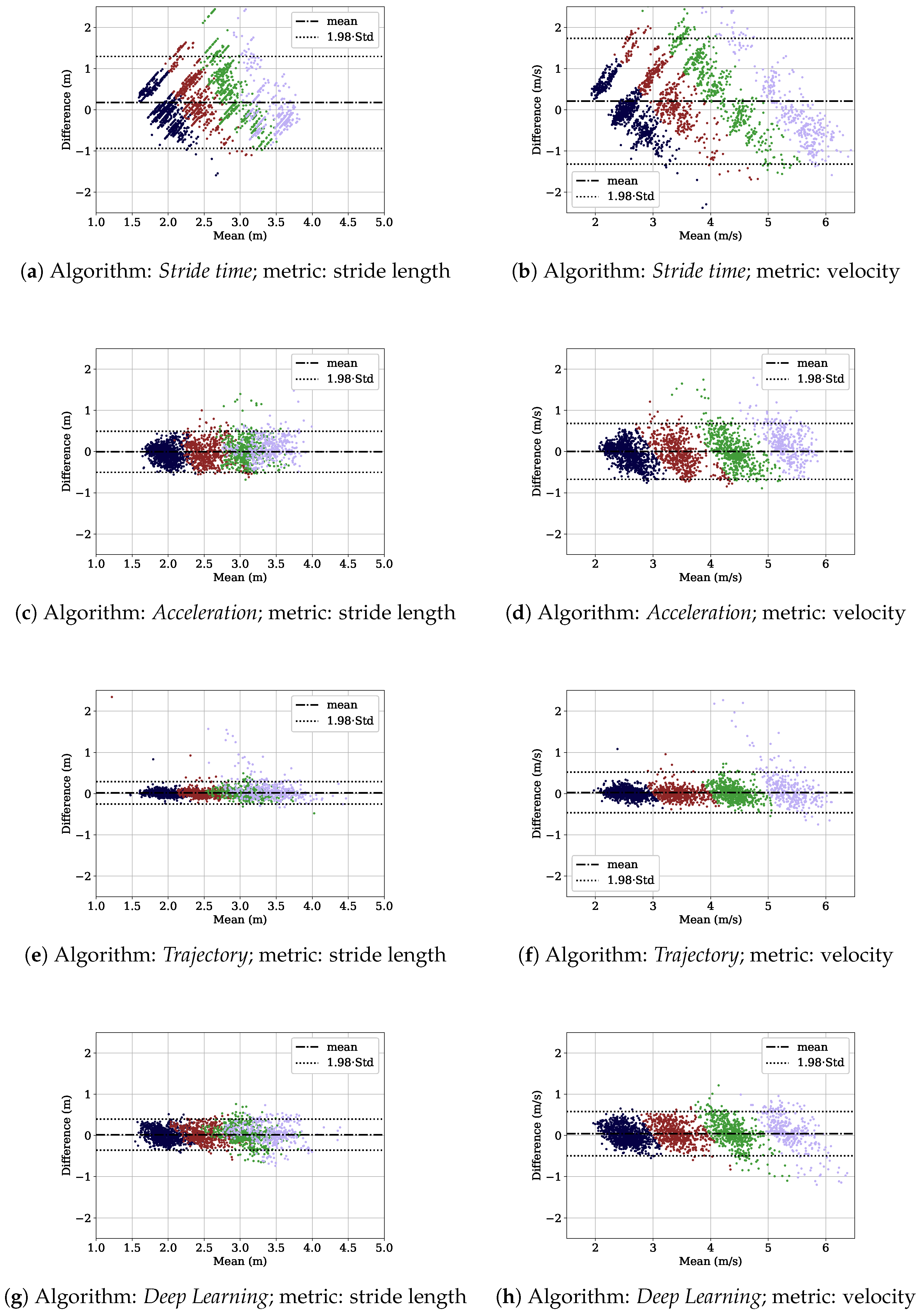
3.1. Lab Study
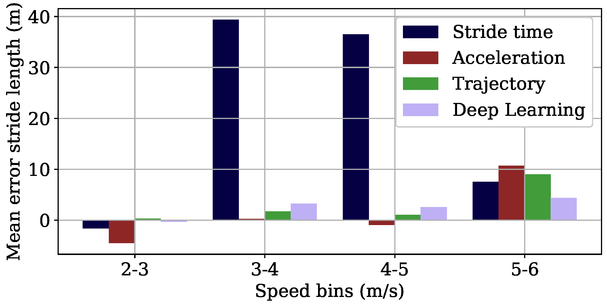
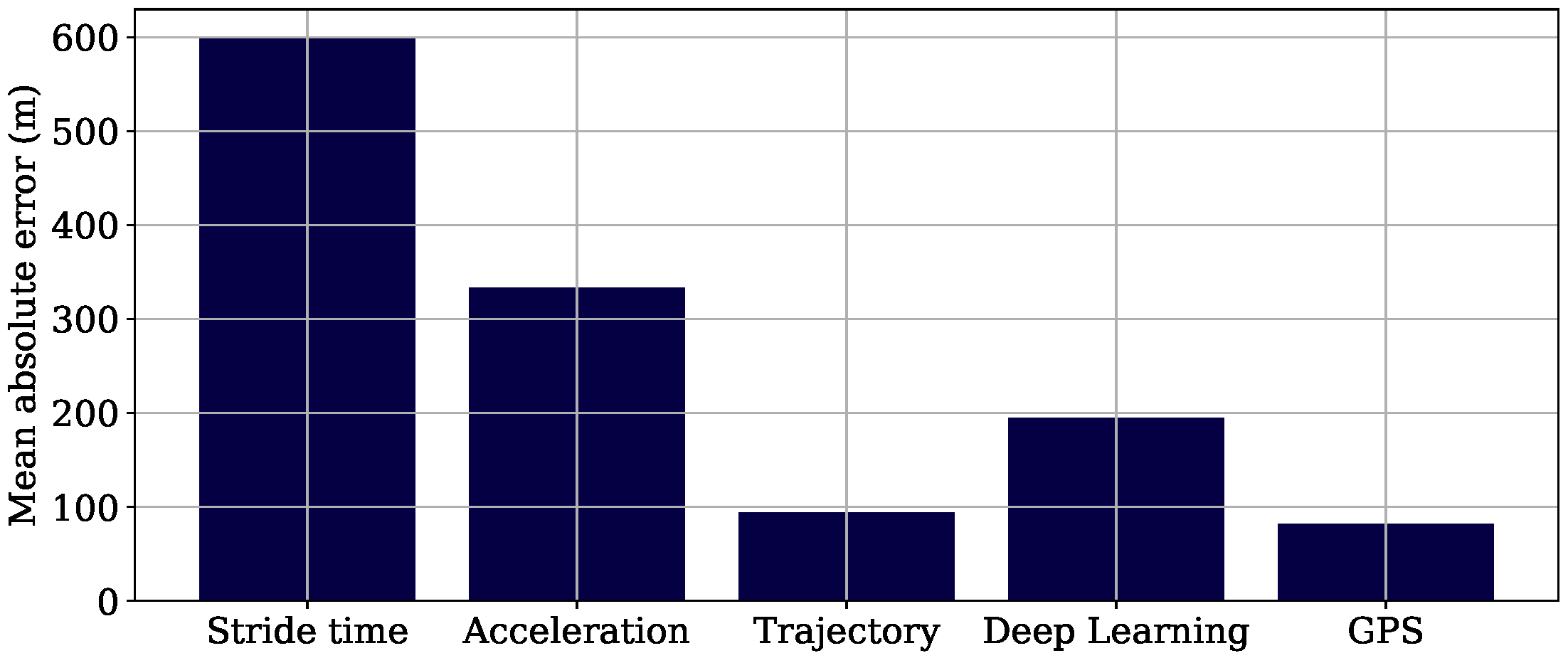
3.2. Field Study
4. Discussion
4.1. Comparison to Existing Literature
4.2. Lab Study
4.3. Field Study
5. Conclusions and Future Work
Author Contributions
Funding
Acknowledgments
Conflicts of Interest
References
- Cornelissen, V.A.; Fagard, R.H. Effects of endurance training on blood pressure, blood pressure—Regulating mechanisms, and cardiovascular risk factors. Hypertension 2005, 46, 667–675. [Google Scholar] [CrossRef] [PubMed]
- Lee, D.C.; Pate, R.R.; Lavie, C.J.; Sui, X.; Church, T.S.; Blair, S.N. Leisure-time running reduces all-cause and cardiovascular mortality risk. J. Am. Coll. Cardiol. 2014, 64, 472–481. [Google Scholar] [CrossRef] [PubMed]
- Gallo, R.A.; Plakke, M.; Silvis, M.L. Common leg injuries of long-distance runners: Anatomical and biomechanical approach. Sports Health 2012, 4, 485–495. [Google Scholar] [CrossRef] [PubMed]
- Mitchell, J.S.; Mount, D.M.; Papadimitriou, C.H. The discrete geodesic problem. SIAM J. Comput. 1987, 16, 647–668. [Google Scholar] [CrossRef]
- Cavanagh, P.R. Biomechanics of Distance Running; Human Kinetics: Champaign, IL, USA, 1990. [Google Scholar]
- Gradl, S.; Zrenner, M.; Schuldhaus, D.; Wirth, M.; Cegielny, T.; Zwick, C. Movement Speed Estimation Based on Foot Acceleration Patterns. In Proceedings of the Annual International Conference of the IEEE Engineering in Medicine and Biology Society, Honolulu, HI, USA, 17–21 July 2018; pp. 3506–3508. [Google Scholar]
- Rampp, A.; Barth, J.; Schuelein, S.; Gassmann, K.G.; Klucken, J.; Eskofier, B.M. Inertial sensor-based stride parameter calculation from gait sequences in geriatric patients. IEEE Trans. Biomed. Eng. 2015, 62, 1089–1097. [Google Scholar] [CrossRef] [PubMed]
- Mariani, B.; Hoskovec, C.; Rochat, S.; Büla, C.; Penders, J.; Aminian, K. 3D gait assessment in young and elderly subjects using foot-worn inertial sensors. J. Biomech. 2010, 43, 2999–3006. [Google Scholar] [CrossRef] [PubMed]
- Ferrari, A.; Ginis, P.; Hardegger, M.; Casamassima, F.; Rocchi, L.; Chiari, L. A mobile Kalman-filter based solution for the real-time estimation of spatio-temporal gait parameters. IEEE Trans. Neural Syst. Rehabil. Eng. 2016, 24, 764–773. [Google Scholar] [CrossRef] [PubMed]
- Bird, J.; Arden, D. Indoor navigation with foot-mounted strapdown inertial navigation and magnetic sensors [emerging opportunities for localization and tracking]. IEEE Wirel. Commun. 2011, 18, 28–35. [Google Scholar] [CrossRef]
- Stroembaeck, P.; Rantakokko, J.; Wirkander, S.L.; Alexandersson, M.; Fors, K.; Skog, I.; Händel, P. Foot-mounted inertial navigation and cooperative sensor fusion for indoor positioning. In Proceedings of the ION International Technical Meeting (ITM), San Diego, CA, USA, 25–27 January 2010; pp. 89–98. [Google Scholar]
- Bailey, G.; Harle, R. Assessment of foot kinematics during steady state running using a foot-mounted IMU. Procedia Eng. 2014, 72, 32–37. [Google Scholar] [CrossRef]
- Foxlin, E. Pedestrian tracking with shoe-mounted inertial sensors. IEEE Comput. Gr. Appl. 2005, 25, 38–46. [Google Scholar] [CrossRef]
- Kautz, T.; Groh, B.H.; Hannink, J.; Jensen, U.; Strubberg, H.; Eskofier, B.M. Activity recognition in beach volleyball using a Deep Convolutional Neural Network. Data Min. Knowl. Discov. 2017, 31, 1678–1705. [Google Scholar] [CrossRef]
- Ordóñez, F.J.; Roggen, D. Deep Convolutional and LSTM Recurrent Neural Networks for Multimodal Wearable Activity Recognition. Sensors 2016, 16, 115. [Google Scholar] [CrossRef] [PubMed]
- Hannink, J.; Kautz, T.; Pasluosta, C.; Barth, J.; Schulein, S.; Gassmann, K.G.; Klucken, J.; Eskofier, B. Mobile Stride Length Estimation with Deep Convolutional Neural Networks. IEEE J. Biomed. Health Inf. 2017, 21, 85–93. [Google Scholar] [CrossRef] [PubMed]
- Altman, A.R.; Davis, I.S. A kinematic method for footstrike pattern detection in barefoot and shod runners. Gait Posture 2012, 35, 298–300. [Google Scholar] [CrossRef] [PubMed] [Green Version]
- Blank, P.; Kugler, P.; Schlarb, H.; Eskofier, B.M. A Wearable Sensor System for Sports and Fitness Applications. In Proceedings of the 19th Annual Congress of the European College of Sport Science, Amsterdam, The Netherlands, 2–5 July 2014; p. 703. [Google Scholar]
- Ferraris, F.; Grimaldi, U.; Parvis, M. Procedure for effortless in-field calibration of three-axial rate gyro and accelerometers. Sens. Mater. 1995, 7, 311–330. [Google Scholar]
- Michel, K.J.; Kleindienst, F.I.; Krabbe, B. Development of a lower extremity model for sport shoe research. In Proceedings of the 13rd Annual Meeting of ESMAC, Warsaw, Poland, 23–25 March 2004; p. 80. [Google Scholar]
- Maiwald, C.; Sterzing, T.; Mayer, T.; Milani, T. Detecting foot-to-ground contact from kinematic data in running. Footwear Sci. 2009, 1, 111–118. [Google Scholar] [CrossRef]
- Kugler, P.; Schlarb, H.; Blinn, J.; Picard, A.; Eskofier, B. A wireless trigger for synchronization of wearable sensors to external systems during recording of human gait. In Proceedings of the Annual International Conference of the IEEE Engineering in Medicine and Biology Society, San Diego, CA, USA, 28 August–1 September 2012; pp. 4537–4540. [Google Scholar]
- Strava Stories—2017 in Stats. 2018. Available online: https://blog.strava.com/2017-in-stats/ (accessed on 22 August 2018).
- GPX—The GPS Exchange Format. Available online: http://www.topografix.com/gpx.asp (accessed on 28 August 2018).
- Karney, C.F. Algorithms for geodesics. J. Geod. 2013, 87, 43–55. [Google Scholar] [CrossRef]
- Strohrmann, C.; Harms, H.; Tröster, G.; Hensler, S.; Müller, R. Out of the lab and into the woods: kinematic analysis in running using wearable sensors. In Proceedings of the 13rd International Conference on Ubiquitous Computing, Beijing, China, 17–21 September 2011; pp. 119–122. [Google Scholar]
- Danion, F.; Varraine, E.; Bonnard, M.; Pailhous, J. Stride variability in human gait: The effect of stride frequency and stride length. Gait Posture 2003, 18, 69–77. [Google Scholar] [CrossRef]
- Perry, J.; Davids, J.R. Gait analysis: Normal and pathological function. J. Pediat. Orthop. 1992, 12, 815. [Google Scholar] [CrossRef]
- Elliott, B.; Blanksby, B. Optimal stride length considerations for male and female recreational runners. Br. J. Sports Med. 1979, 13, 15. [Google Scholar] [CrossRef] [PubMed]
- Hunter, J.P.; Marshall, R.N.; McNair, P.J. Interaction of step length and step rate during sprint running. Med. Sci. Sports Exerc. 2004, 36, 261–271. [Google Scholar] [CrossRef] [PubMed]
- Bailey, G.; Harle, R. Sampling Rates and Sensor Requirements for Kinematic Assessment During Running Using Foot Mounted IMUs. In International Congress on Sports Science Research and Technology Support; Springer: Berlin, Germany, 2014; pp. 42–56. [Google Scholar]
- Skog, I.; Handel, P.; Nilsson, J.O.; Rantakokko, J. Zero-velocity detection—An algorithm evaluation. IEEE Trans. Biomed. Eng. 2010, 57, 2657–2666. [Google Scholar] [CrossRef] [PubMed]
- De Wit, B.; De Clercq, D.; Aerts, P. Biomechanical analysis of the stance phase during barefoot and shod running. J. Biomech. 2000, 33, 269–278. [Google Scholar] [CrossRef]
- LeCun, Y.; Bengio, Y.; Hinton, G. Deep learning. Nature 2015, 521, 436–444. [Google Scholar] [CrossRef] [PubMed]
- Keras. 2015. Available online: https://keras.io (accessed on 22 August 2018).
- Abadi, M.; Agarwal, A.; Barham, P.; Brevdo, E.; Chen, Z.; Citro, C.; Corrado, G.S.; Davis, A.; Dean, J.; Devin, M.; et al. TensorFlow: Large-Scale Machine Learning on Heterogeneous Systems. 2015. Available online: tensorflow.org (accessed on 29 November 2018).
- Srivastava, N.; Hinton, G.E.; Krizhevsky, A.; Sutskever, I.; Salakhutdinov, R. Dropout: A simple way to prevent neural networks from overfitting. J. Mach. Learn. Res. 2014, 15, 1929–1958. [Google Scholar]
- Bland, J.M.; Altman, D. Statistical methods for assessing agreement between two methods of clinical measurement. Lancet 1986, 327, 307–310. [Google Scholar] [CrossRef]
- Lindsay, T.R.; Noakes, T.D.; McGregor, S.J. Effect of treadmill versus overground running on the structure of variability of stride timing. Percept. Mot. Skills 2014, 118, 331–346. [Google Scholar] [CrossRef] [PubMed]
- Abdul Razak, A.H.; Zayegh, A.; Begg, R.K.; Wahab, Y. Foot plantar pressure measurement system: A review. Sensors 2012, 12, 9884–9912. [Google Scholar] [CrossRef] [PubMed] [Green Version]
- MPU-9250 Datasheet. Available online: https://www.invensense.com/download-pdf/mpu-9250-datasheet/ (accessed on 22 August 2018).
- Zrenner, M.; Ullrich, M.; Zobel, P.; Jensen, U.; Laser, F.; Groh, B.; Dümler, B.; Eskofier, B. Kinematic parameter evaluation for the purpose of a wearable running shoe recommendation. In Proceedings of the 15th IEEE International Conference on Wearable and Implantable Body Sensor Networks (BSN), Las Vegas, NV, USA, 4–7 March 2018; pp. 106–109. [Google Scholar]
- Mo, S.; Chow, D.H. Accuracy of three methods in gait event detection during overground running. Gait Posture 2018, 59, 93–98. [Google Scholar] [CrossRef] [PubMed]


| Parameter | Mean ± Standard Deviation |
|---|---|
| Age (years) | |
| Shoe size (U.S.) | |
| Height (cm) |
| Velocity Range | # of Trials | # of Strides |
|---|---|---|
| 2–3 m/s | 10 | 921 |
| 3–4 m/s | 10 | 558 |
| 4–5 m/s | 15 | 544 |
| 5–6 m/s | 15 | 354 |
| (a) Male | (b) Female | ||||
|---|---|---|---|---|---|
| (s) | Reference | (s) | Reference | ||
| 0.830 | [5,27] | 0.826 | [27,28] | ||
| 1.080 | [27,29] | 1.110 | [5,27,29] | ||
| 1.260 | [5] | 1.260 | [5] | ||
| 1.330 | [5] | 1.400 | [5] | ||
| 1.410 | [5] | 1.500 | [5] | ||
| 1.490 | [5] | 1.720 | [5] | ||
| 1.590 | [5] | 1.920 | [5] | ||
| 1.740 | [5] | 2.080 | [5] | ||
| 1.880 | [5] | 2.170 | [30] | ||
| 1.960 | [5] | ||||
| 2.015 | [5] | ||||
| 2.060 | [5] | ||||
| 2.170 | [30] | ||||
| Parameter | Error Measure | Stride Time | Acceleration | Trajectory | Deep Learning |
|---|---|---|---|---|---|
| ME ± Std (m/s) | 0.209 ± 0.782 | 0.005 ± 0.350 | 0.028 ± 0.252 | 0.055 ± 0.285 | |
| Velocity | MAPE (%) | 17.2 | 7.7 | 3.5 | 5.9 |
| MAE (m/s) | 0.622 | 0.272 | 0.133 | 0.216 | |
| ME ± Std (cm) | 17.7 ± 57.3 | −0.5 ± 25.6 | 2.00 ± 14.1 | 2.5 ± 20.1 | |
| Stride length | MAPE (%) | 17.1 | 7.9 | 2.8 | 5.9 |
| MAE (cm) | 45.2 | 19.9 | 7.6 | 15.3 |
| Gait Type | # Subjects | # Strides | Parameter | Error Measure | Result | |
|---|---|---|---|---|---|---|
| Bailey et al. [12] | Running | 5 | 1800 | Velocity | ME | 0.04 ± 0.03 m/s |
| Gradl et al. [6] | Running | 9 | 795 | Velocity | MAPE | 6.9 ± 5.5% |
| Hannink et al. [16] | Walking | 101 | ∼1392 | Stride length | ME | 0.01 ± 5.37 cm |
© 2018 by the authors. Licensee MDPI, Basel, Switzerland. This article is an open access article distributed under the terms and conditions of the Creative Commons Attribution (CC BY) license (http://creativecommons.org/licenses/by/4.0/).
Share and Cite
Zrenner, M.; Gradl, S.; Jensen, U.; Ullrich, M.; Eskofier, B.M. Comparison of Different Algorithms for Calculating Velocity and Stride Length in Running Using Inertial Measurement Units. Sensors 2018, 18, 4194. https://doi.org/10.3390/s18124194
Zrenner M, Gradl S, Jensen U, Ullrich M, Eskofier BM. Comparison of Different Algorithms for Calculating Velocity and Stride Length in Running Using Inertial Measurement Units. Sensors. 2018; 18(12):4194. https://doi.org/10.3390/s18124194
Chicago/Turabian StyleZrenner, Markus, Stefan Gradl, Ulf Jensen, Martin Ullrich, and Bjoern M. Eskofier. 2018. "Comparison of Different Algorithms for Calculating Velocity and Stride Length in Running Using Inertial Measurement Units" Sensors 18, no. 12: 4194. https://doi.org/10.3390/s18124194