A Multisensor Fusion Method for Tool Condition Monitoring in Milling


Abstract
1. Introduction
2. Literature Review
3. Theoretical Framework
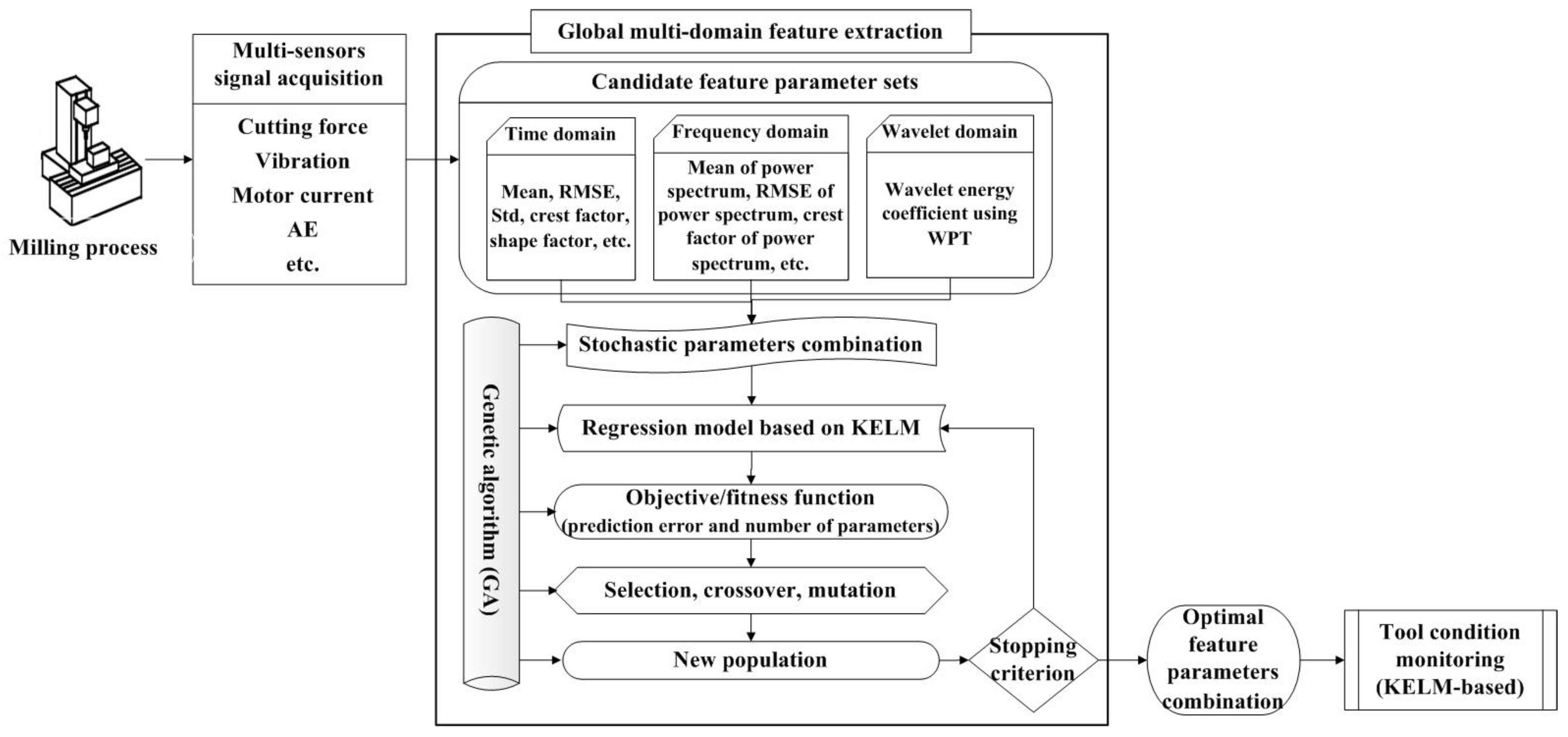
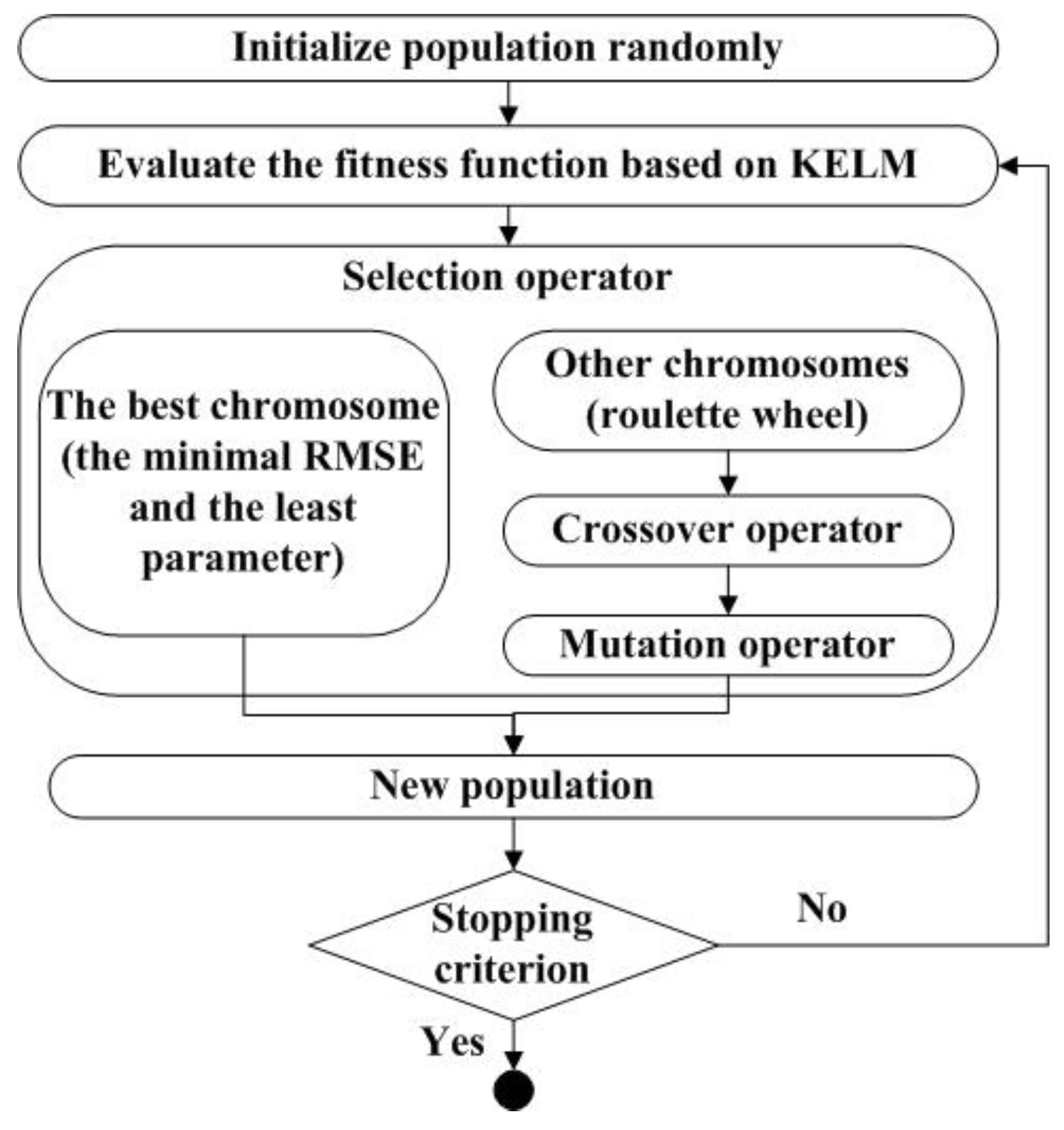
3.1. The Framework of TCM
3.2. Kernel Extreme Learning Machine
3.3. Global Feature Extraction
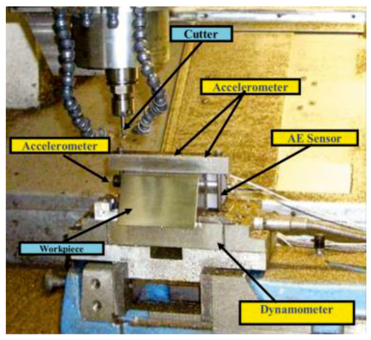
4. Experiments
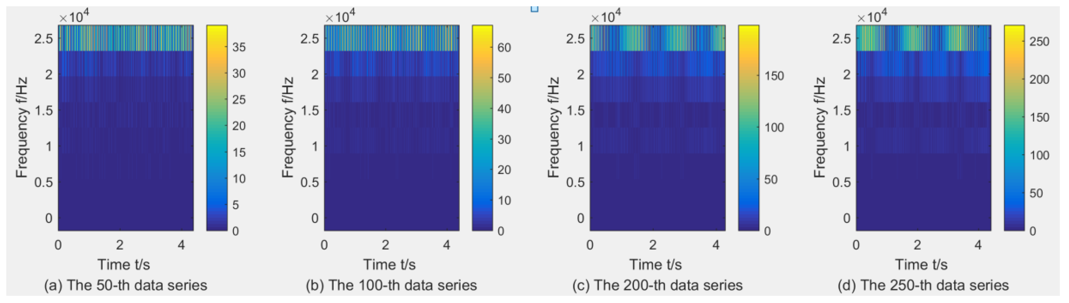
4.1. Descriptions of Datasets
4.2. Candidate Parameter Sets
4.3. Results and Discussion
5. Conclusions
Author Contributions
Funding
Conflicts of Interest
References
- Javed, K.; Gouriveau, R.; Li, X.; Zerhouni, N. Tool wear monitoring and prognostics challenges: A comparison of connectionist methods toward an adaptive ensemble model. J. Intell. Manuf. 2016, 1–18. [Google Scholar] [CrossRef]
- Vetrichelvan, G.; Sundaram, S.; Kumaran, S.S.; Velmurugan, P. An investigation of tool wear using acoustic emission and genetic algorithm. J. Vib. Control 2014, 21, 3061–3066. [Google Scholar] [CrossRef]
- Bhattacharyya, P.; Sengupta, D.; Mukhopadhyay, S. Cutting force-based real-time estimation of tool wear in face milling using a combination of signal processing techniques. Mech. Syst. Signal Process. 2007, 21, 2665–2683. [Google Scholar] [CrossRef]
- Liu, C.; Wang, G.F.; Li, Z.M. Incremental learning for online tool condition monitoring using ellipsoid artmap network model. Appl. Soft Comput. 2015, 35, 186–198. [Google Scholar] [CrossRef]
- Aliustaoglu, C.; Ertunc, H.M.; Ocak, H. Tool wear condition monitoring using a sensor fusion model based on fuzzy inference system. Mech. Syst. Signal Process. 2009, 23, 539–546. [Google Scholar] [CrossRef]
- Konstantinos, S.; Athanasios, K. Reliability assessment of cutting tool life based on surrogate approximation methods. Int. J. Adv. Manuf. Technol. 2014, 71, 1197–1208. [Google Scholar]
- Karandikar, J.; Mcleay, T.; Turner, S.; Schmitz, T. Tool wear monitoring using naïve bayes classifiers. Int. J. Adv. Manuf. Technol. 2015, 77, 1613–1626. [Google Scholar] [CrossRef]
- Gao, R.; Wang, L.; Teti, R.; Dornfeld, D.; Kumara, S.; Mori, M.; Helu, M. Cloud-enabled prognosis for manufacturing. CIRP Ann. 2015, 64, 749–772. [Google Scholar] [CrossRef]
- Rehorn, A.G.; Jiang, J.; Orban, P.E. State-of-the-art methods and results in tool condition monitoring: A review. Int. J. Adv. Manuf. Technol. 2005, 26, 693–710. [Google Scholar] [CrossRef]
- Dutta, S.; Kanwat, A.; Pal, S.K.; Sen, R. Correlation study of tool flank wear with machined surface texture in end milling. Measurement 2013, 46, 4249–4260. [Google Scholar] [CrossRef]
- Ghosh, N.; Ravi, Y.B.; Patra, A.; Mukhopadhyay, S.; Paul, S.; Mohanty, A.R.; Chattopadhyay, A.B. Estimation of tool wear during CNC milling using neural network-based sensor fusion. Mech. Syst. Signal Process. 2007, 21, 466–479. [Google Scholar] [CrossRef]
- Drouillet, C.; Karandikar, J.; Nath, C.; Journeaux, A.C.; Mansori, M.E.; Kurfess, T. Tool life predictions in milling using spindle power with the neural network technique. J. Manuf. Process. 2016, 22, 161–168. [Google Scholar] [CrossRef]
- Chryssolouris, G.; Domroese, M.; Beaulieu, P. Sensor Synthesis for Control of Manufacturing Processes. J. Eng. Ind. ASME 1992, 114, 158–174. [Google Scholar] [CrossRef]
- Nouri, M.; Fussell, B.K.; Ziniti, B.L.; Linder, E. Real-time tool wear monitoring in milling using a cutting condition independent method. Int. J. Mach. Tools Manuf. 2015, 89, 1–13. [Google Scholar] [CrossRef]
- Azmi, A.I. Monitoring of tool wear using measured machining forces and neuro-fuzzy modelling approaches during machining of gfrp composites. Adv. Eng. Softw. 2015, 82, 53–64. [Google Scholar] [CrossRef]
- Zhang, H.; Zhao, J.; Wang, F.; Li, A. Cutting forces and tool failure in high-speed milling of titanium alloy tc21 with coated carbide tools. Proc. Inst. Mech. Eng. Part B J. Eng. Manuf. 2015, 229, 20–27. [Google Scholar] [CrossRef]
- Stavropoulos, P.; Papacharalampopoulos, A.; Vasiliadis, E.; Chryssolouris, G. Tool wear predictability estimation in milling based on multi-sensorial data. Int. J. Adv. Manuf. Technol. 2016, 82, 509–521. [Google Scholar] [CrossRef]
- Snr, D.E.D. Sensor signals for tool-wear monitoring in metal cutting operations—A review of methods. Int. J. Mach. Tools Manuf. 2000, 40, 1073–1098. [Google Scholar]
- Rizal, M.; Ghani, J.A.; Nuawi, M.Z.; Che, H.C.H. A review of sensor system and application in milling process for tool condition monitoring. Res. J. Appl. Sci. Eng. Technol. 2014, 7, 2083–2097. [Google Scholar] [CrossRef]
- Chen, S.L.; Jen, Y.W. Data fusion neural network for tool condition monitoring in cnc milling machining. Int. J. Mach. Tools Manuf. 2000, 40, 381–400. [Google Scholar] [CrossRef]
- Zhou, Y.Q.; Xue, W. Review of tool condition monitoring methods in milling processes. Int. J. Adv. Manuf. Technol. 2018, 96, 2509–2523. [Google Scholar] [CrossRef]
- Zhang, C.; Yao, X.; Zhang, J.; Jin, H. Tool condition monitoring and remaining useful life prognostic based on a wireless sensor in dry milling operations. Sensors 2016, 16, 795. [Google Scholar] [CrossRef] [PubMed]
- Suprock, C.A.; Roth, J.T. Methods for on-line directionally independent failure prediction of end milling cutting tools. Mach. Sci. Technol. 2007, 11, 1–43. [Google Scholar] [CrossRef]
- Huang, P.B.; Ma, C.C.; Kuo, C.H. A PNN self-learning tool breakage detection system in end milling operations. Appl. Soft Comput. 2015, 37, 114–124. [Google Scholar] [CrossRef]
- Cuka, B.; Kim, D.W. Fuzzy logic based tool condition monitoring for end-milling. Robot. Comput.-Integrated Manuf. 2017, 47, 23–36. [Google Scholar] [CrossRef]
- Zhu, K.; Wong, Y.S.; Hong, G.S. Wavelet analysis of sensor signals for tool condition monitoring: A review and some new results. Int. J. Mach. Tools Manuf. 2009, 49, 537–553. [Google Scholar] [CrossRef]
- Madhusudana, C.K.; Kumar, H.; Narendranath, S. Face milling tool condition monitoring using sound signal. Int. J. Syst. Assurance Eng. Manag. 2017, 2017, 1–11. [Google Scholar] [CrossRef]
- Sevilla-Camacho, P.Y.; Robles-Ocampo, J.B.; Jauregui-Correa, J.C.; Jimenez-Villalobos, D. FPGA-based reconfigurable system for tool condition monitoring in high-speed machining process. Measurement 2015, 64, 81–88. [Google Scholar] [CrossRef]
- Liu, C.; Li, Y.; Zhou, G.; Shen, W. A sensor fusion and support vector machine based approach for recognition of complex machining conditions. J. Intell. Manuf. 2016, 1–14. [Google Scholar] [CrossRef]
- Wang, M.; Wang, J. CHMM for tool condition monitoring and remaining useful life prediction. Int. J. Adv. Manuf. Technol. 2012, 59, 463–471. [Google Scholar] [CrossRef]
- Grasso, M.; Albertelli, P.; Colosimo, B.M. An Adaptive SPC Approach for Multi-sensor Fusion and Monitoring of Time-varying Processes. Procedia Cirp 2013, 12, 61–66. [Google Scholar] [CrossRef]
- Wang, G.; Zhang, Y.; Liu, C.; Xie, Q.; Xu, Y. A new tool wear monitoring method based on multi-scale pca. J. Intell. Manuf. 2016, 7, 1–10. [Google Scholar] [CrossRef]
- Wang, G.F.; Yang, Y.W.; Zhang, Y.C.; Xie, Q.L. Vibration sensor based tool condition monitoring using ν, support vector machine and locality preserving projection. Sens. Actuators A Phys. 2014, 209, 24–32. [Google Scholar] [CrossRef]
- Wang, J.; Xie, J.; Zhao, R.; Zhang, L.; Duan, L. Multisensory fusion based virtual tool wear sensing for ubiquitous manufacturing. Robot. Comput. Integr. Manuf. 2017, 45, 47–58. [Google Scholar] [CrossRef]
- Wang, G.; Yang, Y.; Li, Z. Force sensor based tool condition monitoring using a heterogeneous ensemble learning model. Sensors 2014, 14, 21588–21602. [Google Scholar] [CrossRef] [PubMed]
- Cho, S.; Binsaeid, S.; Asfour, S. Design of multisensor fusion-based tool condition monitoring system in end milling. Int. J. Adv. Manuf. Technol. 2010, 46, 681–694. [Google Scholar] [CrossRef]
- Huang, G.B.; Zhou, H.; Ding, X.; Zhang, R. Extreme learning machine for regression and multiclass classification. IEEE Trans. Syst. Man Cybern. Part B 2012, 42, 513–529. [Google Scholar] [CrossRef] [PubMed]
- Huang, G.B. What are Extreme Learning Machines? Filling the Gap Between Frank Rosenblatt’s Dream and John von Neumann’s Puzzle. Cognit. Comput. 2015, 7, 263–278. [Google Scholar] [CrossRef]
- Chen, X.; Peng, X.; Li, J.; Peng, Y. Overview of Deep Kernel Learning Based Techniques and Applications. J. Netw. Intell. 2016, 1, 83–98. [Google Scholar]
- Maslov, I.V.; Gertner, I. Multi-sensor fusion: An Evolutionary algorithm approach. Inf. Fusion 2006, 7, 304–330. [Google Scholar] [CrossRef]
- The Prognostics and Health Management Society, 2010 Conference Data Challenge. Available online: https://www.phmsociety.org/competition/phm/10 (accessed on 1 June 2018).
- Benkedjouh, T.; Zerhouni, N.; Rechak, S. Tool wear condition monitoring based on continuous wavelet transform and blind source separation. Int. J. Adv. Manuf. Technol. 2018, 97, 3311–3323. [Google Scholar] [CrossRef]
- Zhou, Y.; Liu, X.; Li, F.; Bingtao, S.; Wei, X. An online damage identification approach for numerical control machine tools based on data fusion using vibration signals. J. Vib. Control 2015, 21, 2925–2936. [Google Scholar]
- Zhao, R.; Yan, R.; Wang, J.; Mao, K. Learning to Monitor Machine Health with Convolutional Bi-Directional LSTM Networks. Sensors 2017, 17, 273. [Google Scholar] [CrossRef] [PubMed]
- Gao, C.; Xue, W.; Ren, Y.; Zhou, Y. Numerical control machine tool fault diagnosis using hybrid stationary subspace analysis and least squares support vector machine with a single sensor. Appl. Sci. 2017, 7, 346. [Google Scholar] [CrossRef]
- Zhao, R.; Wang, D.; Yan, R.; Mao, K.; Shen, F.; Wang, J. Machine Health Monitoring Using Local Feature-based Gated Recurrent Unit Networks. IEEE Trans. Ind. Electron. 2017, 65, 1539–1548. [Google Scholar] [CrossRef]
- Chen, B.; Chen, X.; Li, B.; He, Z.; Cao, H.; Cai, G. Reliability estimation for cutting tools based on logistic regression model using vibration signals. Noise Vib. Bull. 2011, 25, 2526–2537. [Google Scholar] [CrossRef]
- Wang, G.; Grosu, R. Milling-tool wear-condition prediction with statistic analysis and echo-state networks. Challenges Technol. Innov. 2017, 149–153. [Google Scholar]


| Operation Parameter | Value |
|---|---|
| CNC machine | Roders Tech RFM 760 |
| Workpiece material | Inconel 718 (Jet engines) |
| Cutter | 3-flute ball nose |
| Spindle speed | 10,400 RPM |
| Feed rate | 1555 mm/min |
| Y depth of cut (radial) | 0.125 mm |
| Z depth of cut (axial) | 0.2 mm |
| Number of sensors | 5 |
| Number of sensor channels | 7 |
| Sampling data | 50 KHz/channel |
| Domain | Indexes | Formula |
|---|---|---|
| Time | Average Value Tavg | |
| Root mean square Trms | ||
| Standard Deviation Tsd | ||
| Crest Factor Tcf | ||
| Shape factor Tsf | ||
| Waveform Twf | ||
| Kurtosis Factor Tku | ||
| Skewness Factor Tsk | ||
| Margin factor Tmf |
| Domain | Indexes | Formula |
|---|---|---|
| Frequency | Mean of power spectrum Fmps | |
| Root mean square of power spectrum Frms | ||
| Crest factor of power spectrum Fcf | ||
| Modified equivalent bandwidth Fmeb | ||
| High–low ratio of power spectrum Fhlps | ||
| Stabilization ratio Fsr | ||
| Skewness of bandpower Fsb | ||
| Kurtosis of bandpower Fkb |
| Parameters | Value |
|---|---|
| Size of the population for every generation | 50 |
| Crossover rate Pc | 0.6 |
| Mutation rate Pm | 0.05 |
| Number of iterations | 1500 |
| Regularization parameter C | 6 |
| Kernel function | Gaussion kernel |
| Hyperparameter of kernel | 2 |
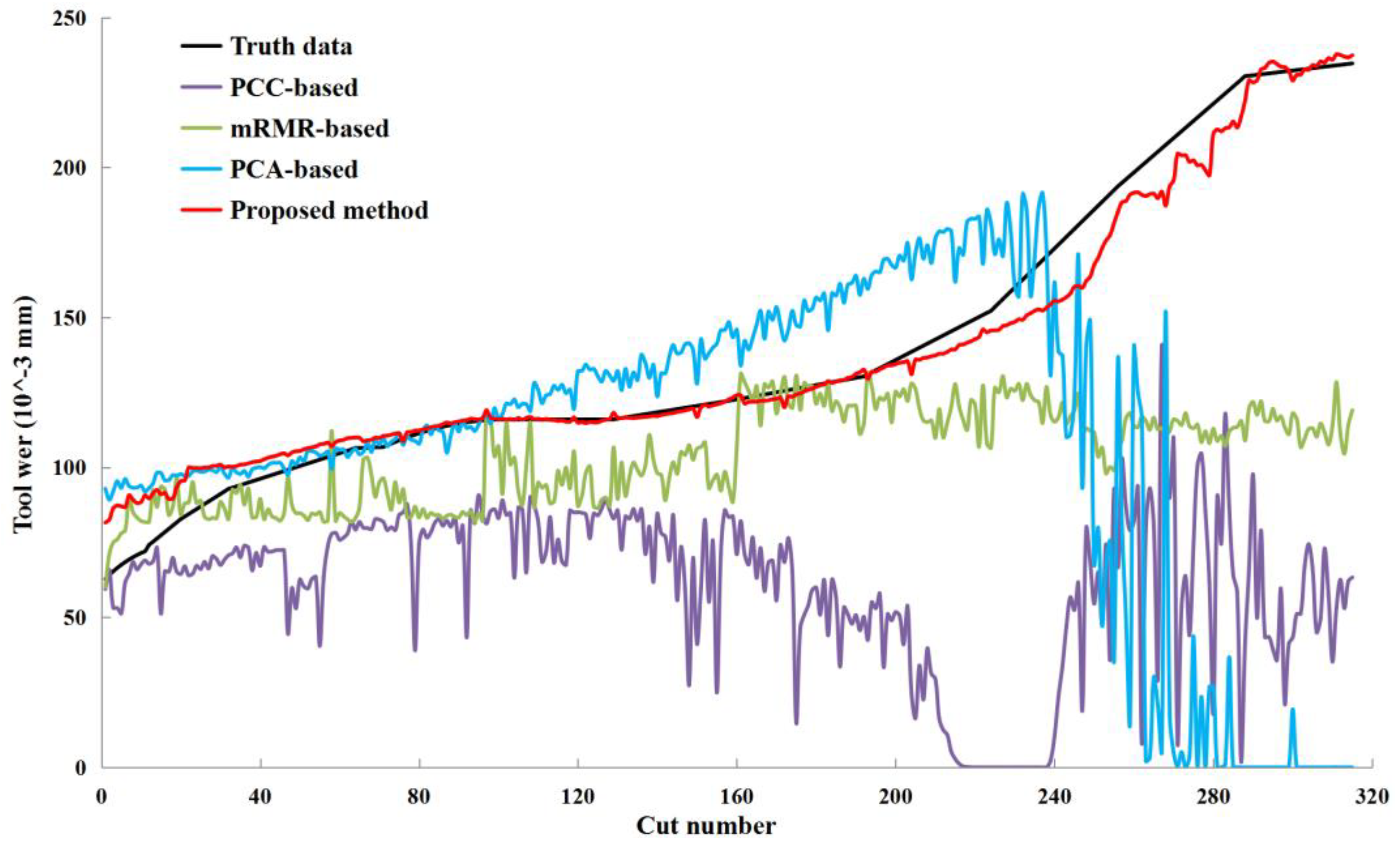
| Methods | RMSE | R2 | Number of Selected Parameters | Number of Sensor Channels Involved |
|---|---|---|---|---|
| The PCC-based method | 98.339 | −0.198 | 33 | 5 |
| The PCA-based method | 94.665 | −0.5768 | 175 | 7 |
| The mRMR-based method | 53.268 | 0.598 | 19 | 5 |
| The proposed method | 24.711 | 0.988 | 11 | 2 |
© 2018 by the authors. Licensee MDPI, Basel, Switzerland. This article is an open access article distributed under the terms and conditions of the Creative Commons Attribution (CC BY) license (http://creativecommons.org/licenses/by/4.0/).
Share and Cite
Zhou, Y.; Xue, W. A Multisensor Fusion Method for Tool Condition Monitoring in Milling. Sensors 2018, 18, 3866. https://doi.org/10.3390/s18113866
Zhou Y, Xue W. A Multisensor Fusion Method for Tool Condition Monitoring in Milling. Sensors. 2018; 18(11):3866. https://doi.org/10.3390/s18113866
Chicago/Turabian StyleZhou, Yuqing, and Wei Xue. 2018. "A Multisensor Fusion Method for Tool Condition Monitoring in Milling" Sensors 18, no. 11: 3866. https://doi.org/10.3390/s18113866
APA StyleZhou, Y., & Xue, W. (2018). A Multisensor Fusion Method for Tool Condition Monitoring in Milling. Sensors, 18(11), 3866. https://doi.org/10.3390/s18113866