Context Impacts in Accelerometer-Based Walk Detection and Step Counting


Abstract
1. Introduction
2. Take Context into Consideration
2.1. Context Definition
2.2. Related Works on Context Impacts
- (1)
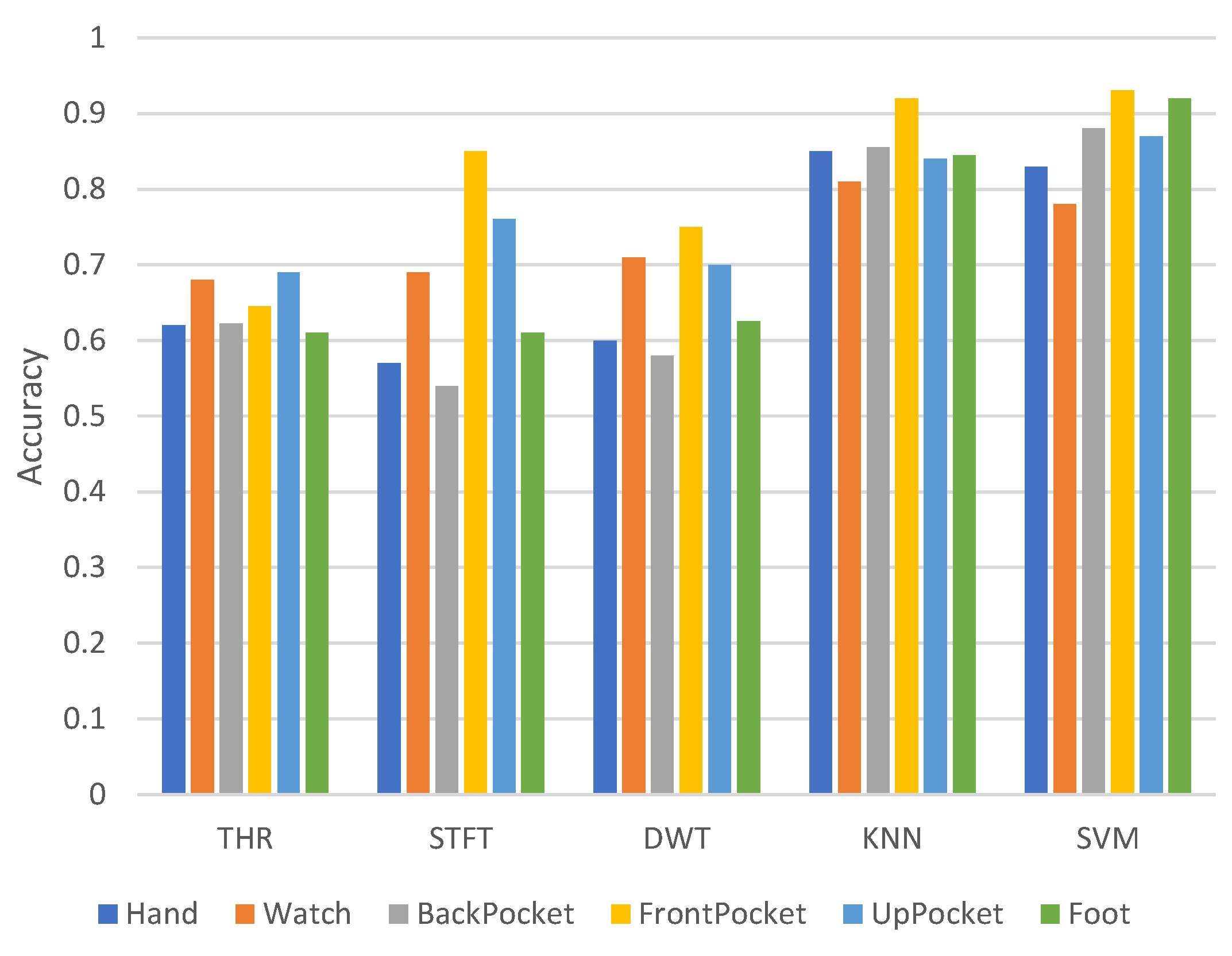
- Placement is the most common context and is the factor that has attracted researchers’ attention. Olguin et al. placed one or two accelerometers on three different parts of the body and studied the classification accuracy of activity recognition [17]. Lester et al. studied whether a single accelerometer could generalize well on different locations and the reliability of activity recognition on a novel individual [18]. The works in [2,19] explored the influences of placements on different body parts. The work in [1,3] showed that the negative influence of various placements of the sensor could be mitigated. Cleland et al. studied the optimal placement to detect daily activities [20]. Sun et al. investigated the effects of varying positions and orientations on the accuracy of activity recognition [21].
- (2)
- The impact of personalization was investigated in [22]. The work in [22] compared the impersonal model and personal model. The impersonal model was built using the data from many users and tested on a new user; the personal model was a personalized method built with the data from the specified user and tested on him/herself. The result showed that the personalized method was much better than the impersonal model. By using active learning and semi-supervised learning algorithms, [23,24] in fact developed a personalized model based on a original classifier and showed the significant improvement over the original classifier, which was trained on the data from many users.
- (3)
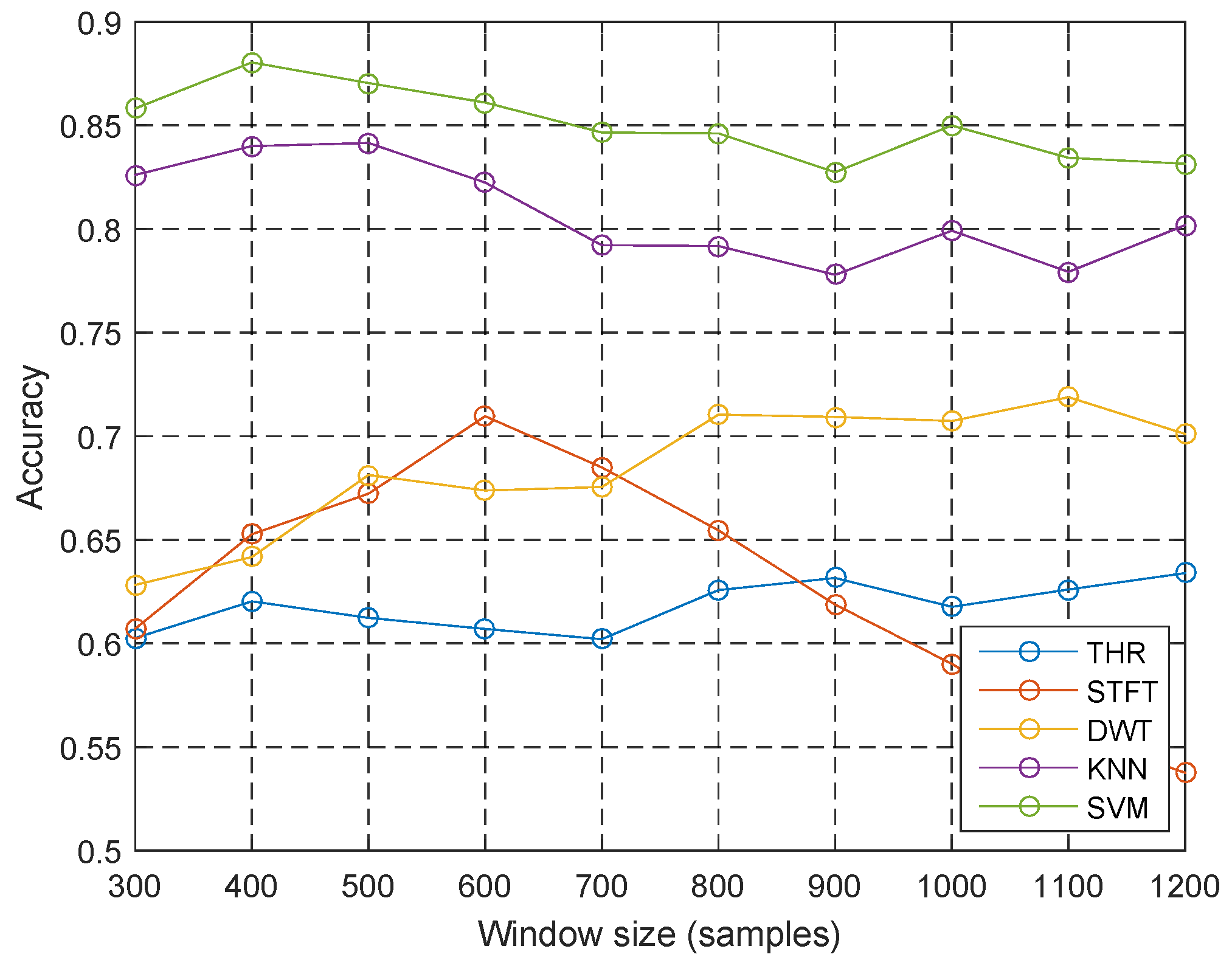
- The impacts of window size were evaluated in [21,25,26]. Although [25] demonstrated that the accuracy was nearly the same under different window sizes, these findings contradicted those of [21,26]. The main reason is that the contexts of the three works were different, which shows the importance of conducting complete evaluations under various contexts.
- (4)
- The impacts of multiple contexts were also investigated in some existing works. The work in [3] investigated the placements, feature selection and the window on/off on the accelerator to evaluate the accuracy of activity recognition. The research showed that the accuracy at the trouser front pocket position had lower accuracy to classify activities and also had difficulty in distinguishing normal walking and fast walking. In addition, the work showed that the classification accuracy between standing and sitting could be significantly enhanced if the sensor position were considered.
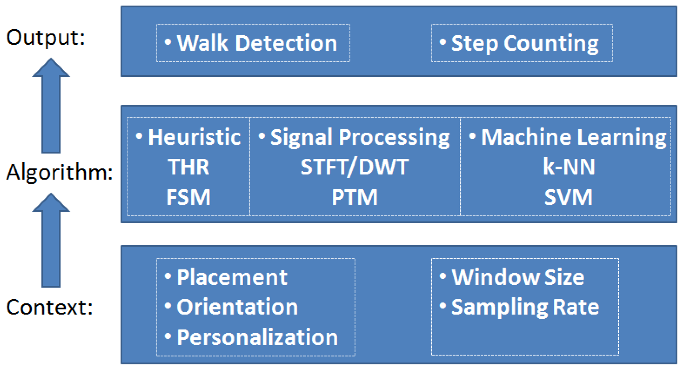
3. WD and SC Algorithms
3.1. Feature Extraction Techniques
3.2. Related Algorithms
3.2.1. Heuristic Methods
3.2.2. Signal Processing Methods
3.2.3. Machine Learning Methods
3.3. Selected Algorithms for Comparison
4. Experiment Design
4.1. Experiment Settings
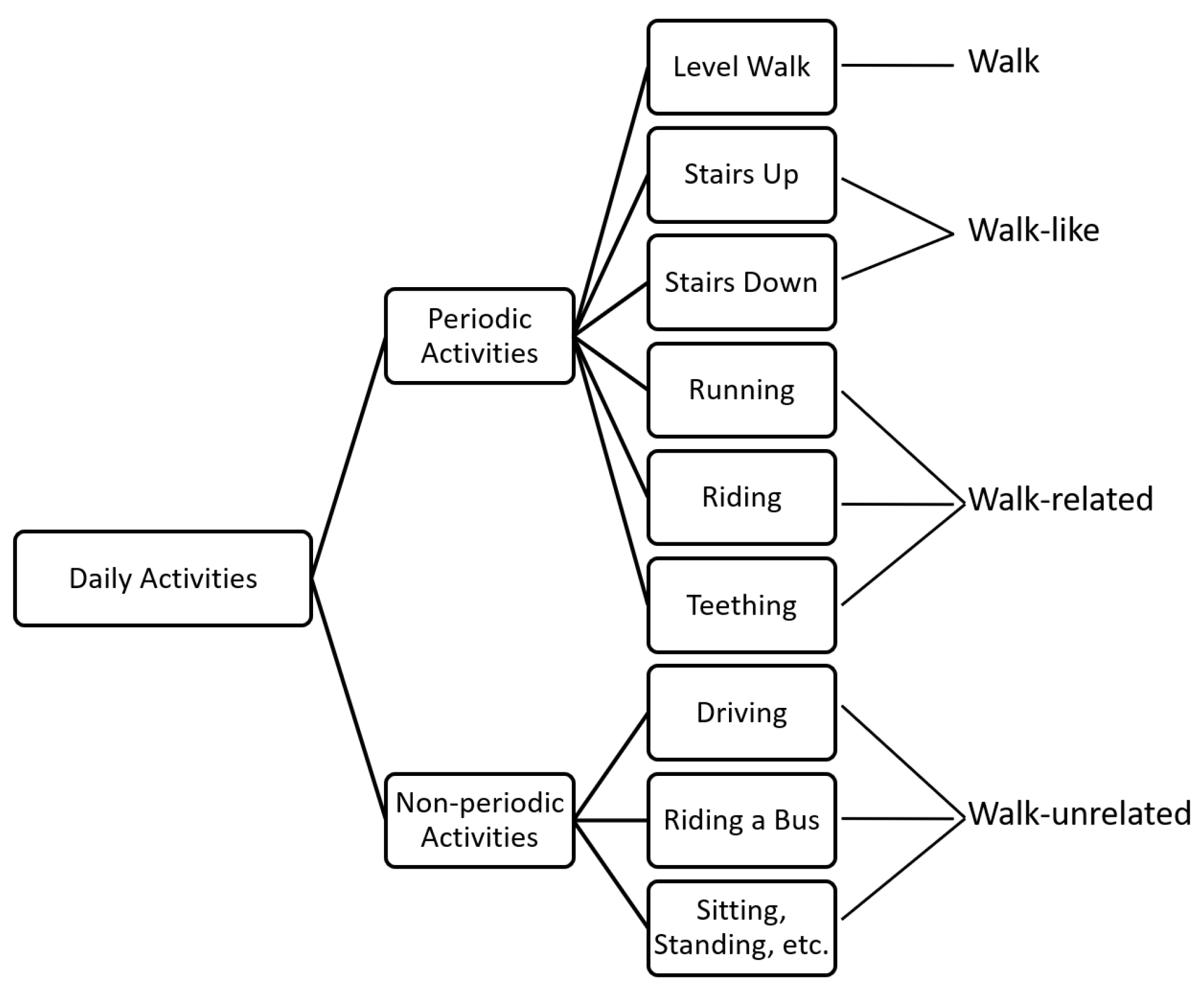
4.1.1. User Activity Categorization
4.1.2. Problem Simplification
- -
- Sample data at 200 Hz, which is nearly the highest sampling rate of most devices, and downsample it to the evaluation.
- -
- Carry one or two devices at one time and repeat it to cover all the six placements defined in Table 3, since the acceleration data in consecutive rounds within a same building are similar.
- -
- Device orientation of the same placement across different subjects is the same.
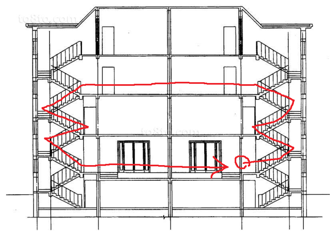
4.1.3. Experiment Scheme
4.2. Data Pre-Processing
4.3. Feature Extraction
4.4. Algorithm Parameter Setting
4.5. Counting
5. Evaluation Results
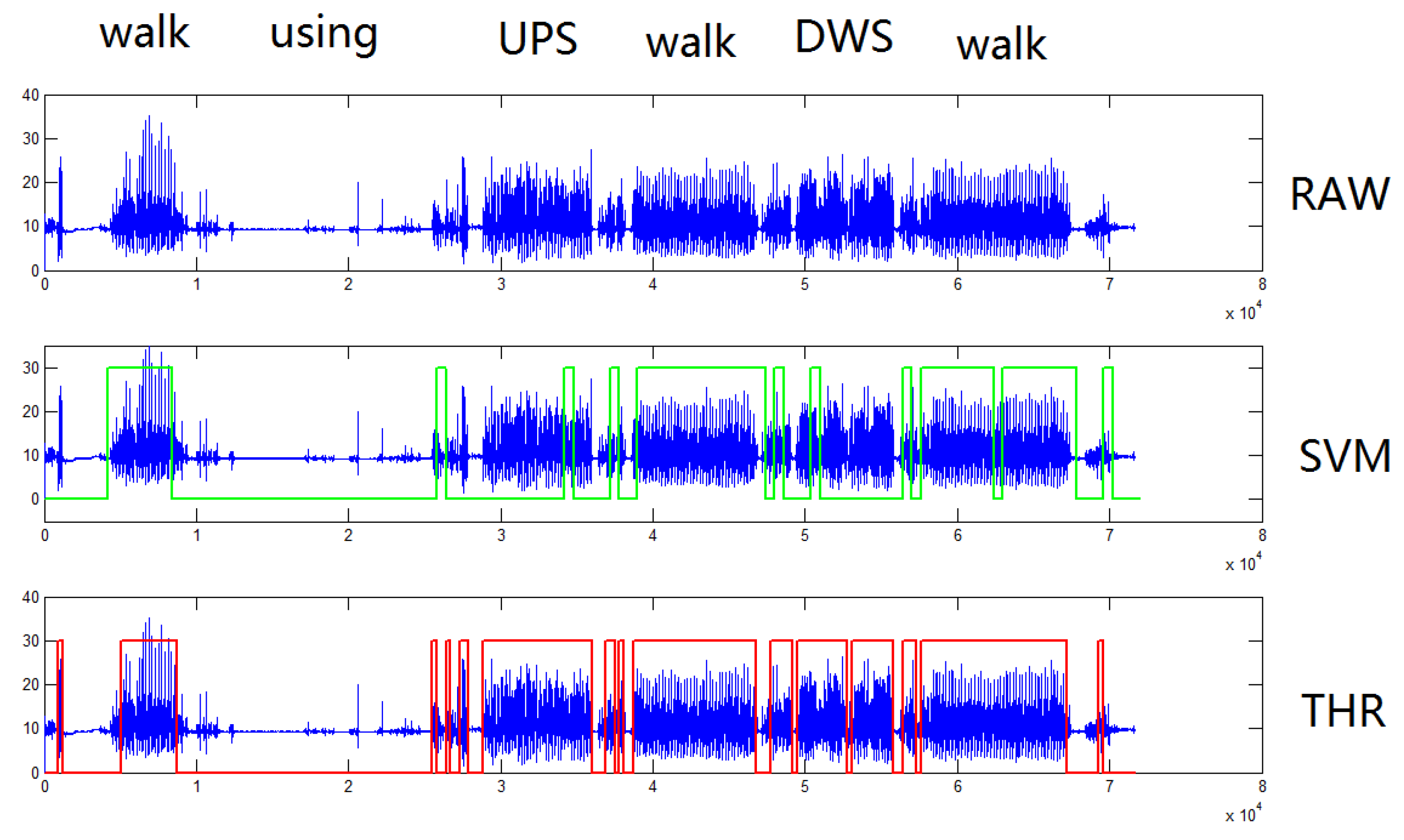
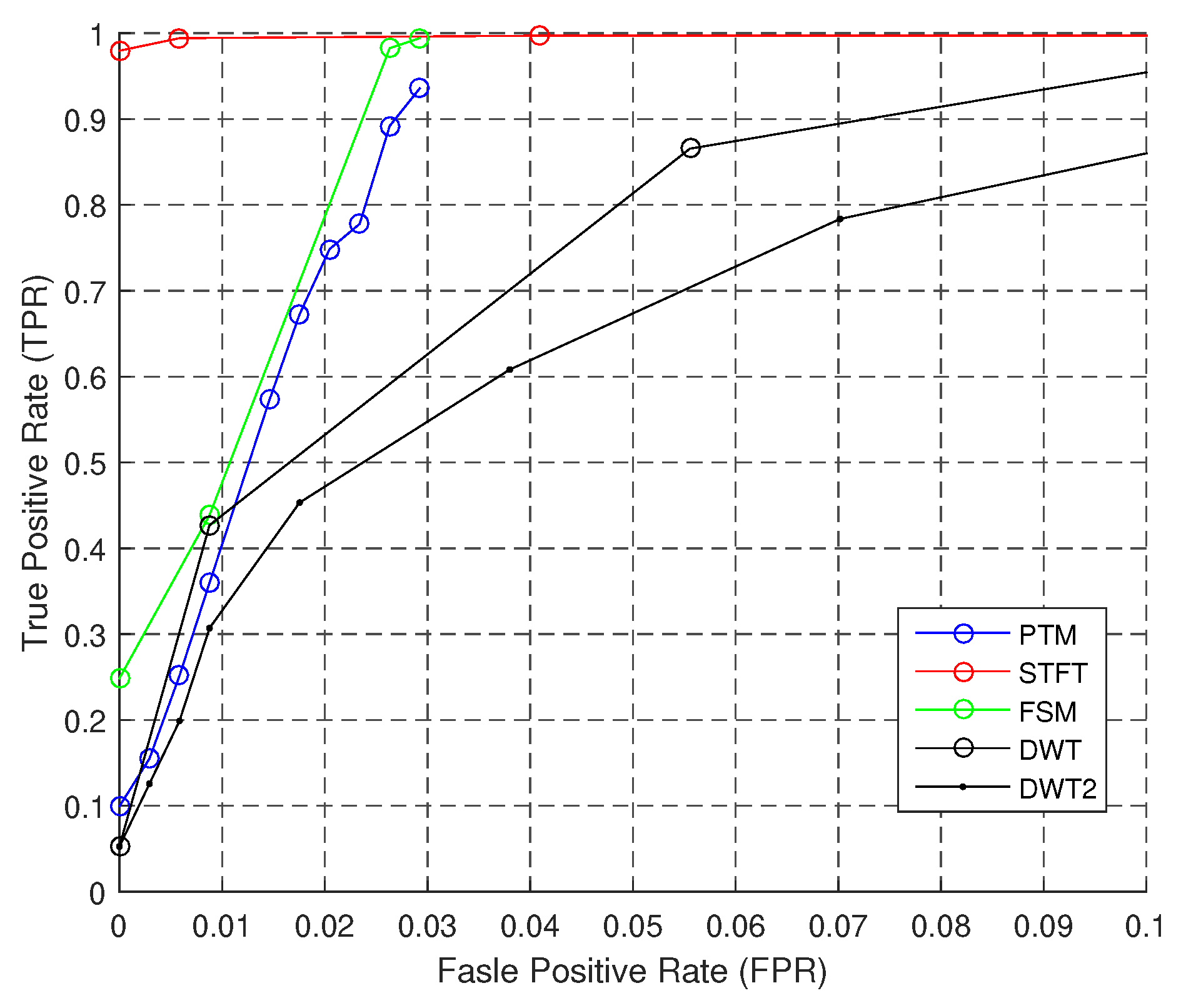
5.1. Coarse-Grained WD
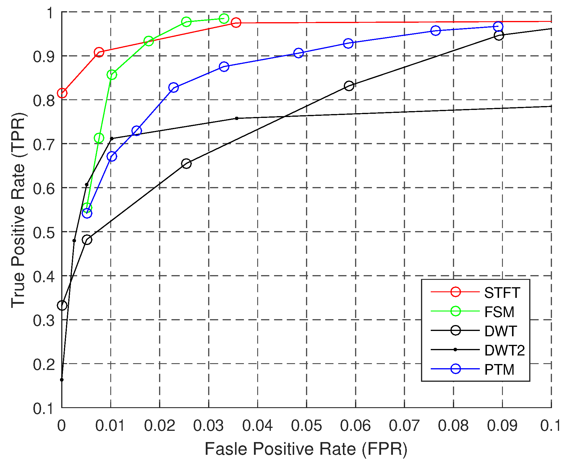
5.2. Context Impacts on Fine-Grained WD
5.2.1. Baseline Performance
5.2.2. Context Effects
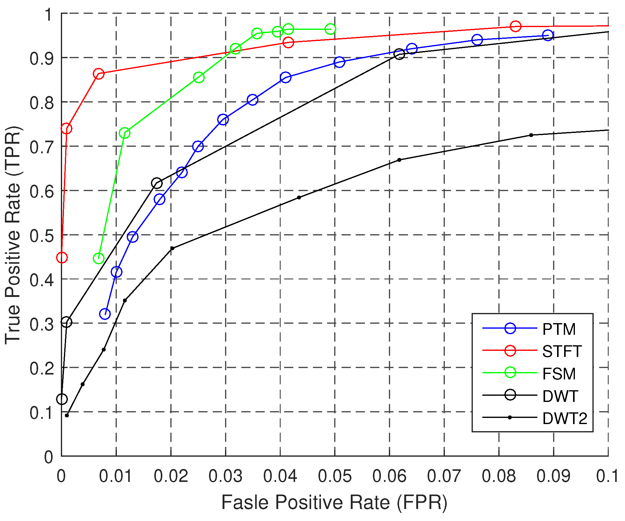
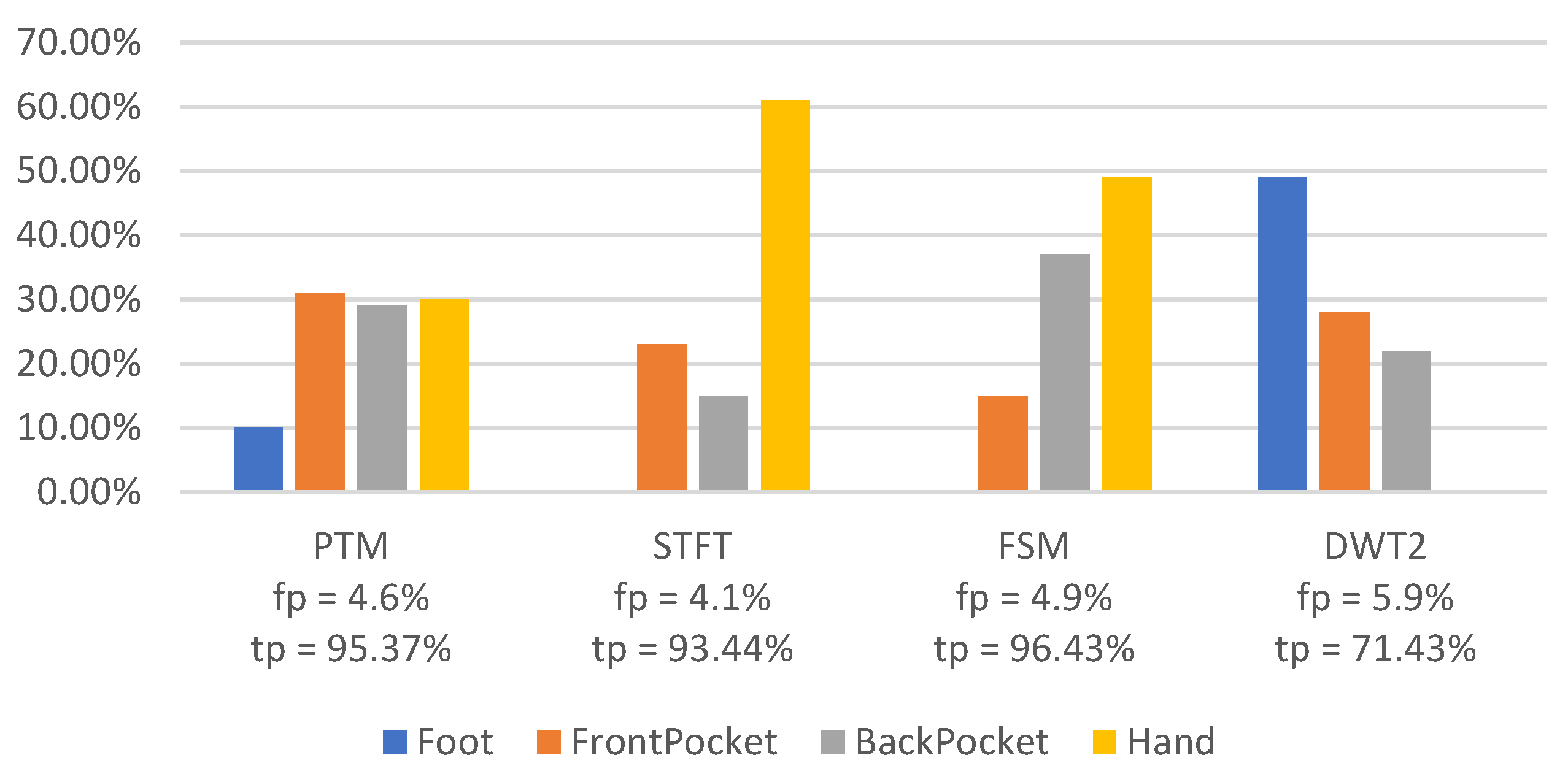
5.3. Context Impacts on SC
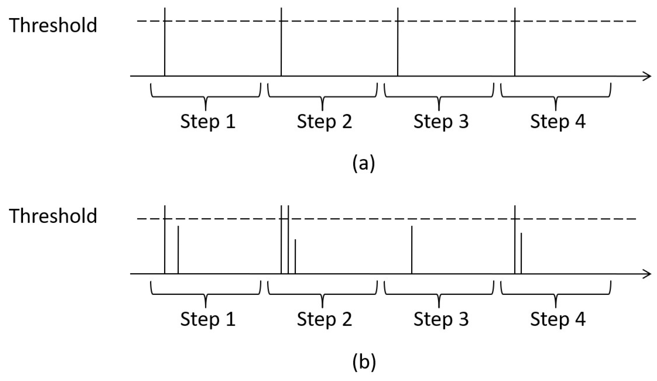
5.3.1. Definition
5.3.2. Baseline Performance
5.3.3. Context Effects
5.4. Design Rules
- -
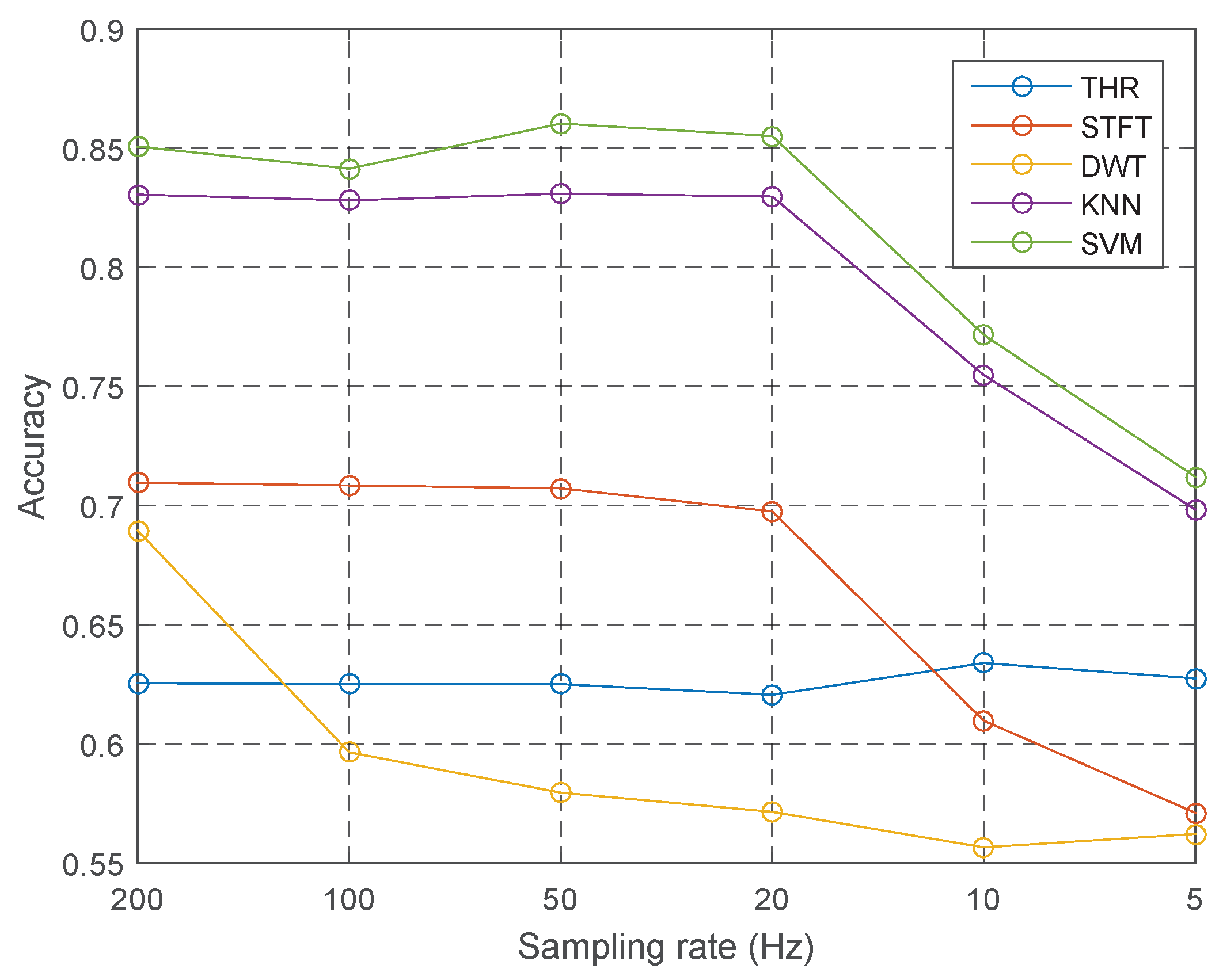
- Although machine learning methods perform best overall, STFT could achieve an acceptable level of accuracy when we detect walk and walk-like activity from the other two activities; 20 Hz is the transition point of the sampling rate.
- -
- Among all the contexts, personal info is most contributive where the model is trained on a specific person.
- -
- Complex does not mean accurate: in SC, STFT and FSM perform better in most test cases; PTM is trivial; and DWT overall performs less productive comparatively except at Hand.
- -
- If sensors are mounted on foot, then the noise is minimal, and the result is most reliable.
- -
- Although the steps are accurate, they may suffer from miss counting and false positives; please see the strict definition of SC.
6. Conclusions
Author Contributions
Funding
Acknowledgments
Conflicts of Interest
References
- Kunze, K. Compensating for on-Body Placement Effects in Activity Recognition. Ph.D. Thesis, University Library Passau, Passau, Germany, 2011. [Google Scholar]
- Kunze, K.; Lukowicz, P. Sensor Placement Variations in Wearable Activity Recognition. IEEE Pervasive Comput. 2014, 13, 32–41. [Google Scholar] [CrossRef]
- Martín, H.; Bernardos, A.M.; Iglesias, J.; Casar, J.R. Activity Logging Using Lightweight Classification Techniques in Mobile Devices. Pers. Ubiquitous Comput. 2013, 17, 675–695. [Google Scholar] [CrossRef]
- Brajdic, A.; Harle, R. Walk Detection and Step Counting on Unconstrained Smartphones. In Proceedings of the 2013 ACM International Joint Conference on Pervasive and Ubiquitous Computing, Zurich, Switzerland, 8–12 September 2013; ACM: New York, NY, USA, 2013; pp. 225–234. [Google Scholar] [CrossRef]
- Bulling, A.; Blanke, U.; Schiele, B. A Tutorial on Human Activity Recognition Using Body-worn Inertial Sensors. ACM Comput. Surv. 2014, 46, 33. [Google Scholar] [CrossRef]
- Zhang, M.; Sawchuk, A.A. USC-HAD: A daily activity dataset for ubiquitous activity recognition using wearable sensors. In Proceedings of the 2012 ACM Conference on Ubiquitous Computing, Pittsburgh, PA, USA, 5–8 September 2012. [Google Scholar]
- Anguita, D.; Ghio, A.; Oneto, L.; Parra, X.; Reyes-Ortiz, J.L. A Public Domain Dataset for Human Activity Recognition Using Smartphones. In Proceedings of the European Symposium on Artificial Neural Networks, Computational Intelligence and Machine Learning, Bruges, Belgium, 24–26 April 2013. [Google Scholar]
- Bruno, B.; Mastrogiovanni, F.; Sgorbissa, A.; Vernazza, T.; Zaccaria, R. Analysis of human behavior recognition algorithms based on acceleration data. In Proceedings of the 2013 IEEE International Conference on Robotics and Automation, Karlsruhe, Germany, 6–10 May 2013; pp. 1602–1607. [Google Scholar]
- Kwapisz, J.R.; Weiss, G.M.; Moore, S.A. Activity Recognition Using Cell Phone Accelerometers. ACM SigKDD Explor. Newsl. 2011, 12, 74–82. [Google Scholar] [CrossRef]
- Tapia, E.M.; Intille, S.S.; Lopez, L.; Larson, K. The Design of a Portable Kit of Wireless Sensors for Naturalistic Data Collection. In Proceedings of the International Conference on Pervasive Computing, Dublin, Ireland, 7–10 May 2006. [Google Scholar]
- Collecting complex activity datasets in highly rich networked sensor environments. In Proceedings of the 2010 Seventh International Conference on Networked Sensing Systems (INSS), Kassel, Germany, 15–18 June 2010.
- Zheng, Y.; Shen, G.; Li, L.; Zhao, C.; Li, M.; Zhao, F. Travi-navi: Self-deployable indoor navigation system. IEEE/ACM Trans. Netw. 2017, 25, 2655–2669. [Google Scholar] [CrossRef]
- Wannenburg, J.; Malekian, R. Physical activity recognition from smartphone accelerometer data for user context awareness sensing. IEEE Trans. Syst. Man Cybern. Syst. 2017, 47, 3142–3149. [Google Scholar] [CrossRef]
- Delgado-Gonzalo, R.; Hubbard, J.; Renevey, P.; Lemkaddem, A.; Vellinga, Q.; Ashby, D.; Willardson, J.; Bertschi, M. Real-time gait analysis with accelerometer-based smart shoes. In Proceedings of the 2017 39th Annual International Conference of the IEEE Engineering in Medicine and Biology Society (EMBC), Seogwipo, Korea, 11–15 July 2017; p. 148. [Google Scholar]
- de la Concepción, M.Á.Á.; Morillo, L.M.S.; García, J.A.Á.; González-Abril, L. Mobile activity recognition and fall detection system for elderly people using Ameva algorithm. Pervasive Mob. Comput. 2017, 34, 3–13. [Google Scholar] [CrossRef]
- Cheng, J.; Yang, L.; Li, Y.; Zhang, W. Seamless outdoor/indoor navigation with WIFI/GPS aided low cost Inertial Navigation System. Phys. Commun. 2014, 13, 31–43. [Google Scholar] [CrossRef]
- Olguın, D.O.; Pentland, A.S. Human activity recognition: Accuracy across common locations for wearable sensors. In Proceedings of the 2006 10th IEEE International Symposium on Wearable Computers, Montreux, Switzerland, 11–14 October 2006. [Google Scholar]
- Lester, J.; Choudhury, T.; Borriello, G. A practical approach to recognizing physical activities. In Proceedings of the Pervasive Computing, Dublin, Ireland, 7–10 May 2006; Springer: Berlin/Heidelberg, Germany, 2006; pp. 1–16. [Google Scholar]
- Pärkkä, J.; Cluitmans, L.; Ermes, M. Personalization Algorithm for Real-Time Activity Recognition Using PDA, Wireless Motion Bands, and Binary Decision Tree. IEEE Trans. Inf. Technol. Biomed. 2010, 14, 1211–1215. [Google Scholar] [CrossRef] [PubMed]
- Cleland, I.; Kikhia, B.; Nugent, C.; Boytsov, A.; Hallberg, J.; Synnes, K.; McClean, S.; Finlay, D. Optimal placement of accelerometers for the detection of everyday activities. Sensors 2013, 13, 9183–9200. [Google Scholar] [CrossRef] [PubMed]
- Sun, L.; Zhang, D.; Li, B.; Guo, B.; Li, S. Activity recognition on an accelerometer embedded mobile phone with varying positions and orientations. In Proceedings of the International Conference on Ubiquitous Intelligence and Computing, Xi’an, China, 26–29 October 2010; Springer: Berlin/Heidelberg, Germany; pp. 548–562. [Google Scholar]
- Weiss, G.M.; Lockhart, J.W. The impact of personalization on smartphone-based activity recognition. In Proceedings of the AAAI Workshops at the Twenty-Sixth AAAI Conference on Artificial Intelligence, Toronto, ON, Canada, 22–26 July 2012. [Google Scholar]
- Longstaff, B.; Reddy, S.; Estrin, D. Improving activity classification for health applications on mobile devices using active and semi-supervised learning. In Proceedings of the 2010 4th International Conference on Pervasive Computing Technologies for Healthcare, Munich, Germany, 22–25 March 2010; pp. 1–7. [Google Scholar] [CrossRef]
- Hong, J.H.; Ramos, J.; Dey, A.K. Toward Personalized Activity Recognition Systems with a Semipopulation Approach. IEEE Trans. Hum.-Mach. Syst. 2016, 46, 101–112. [Google Scholar] [CrossRef]
- Harasimowicz, A.; Dziubich, T.; Brzeski, A. Accelerometer-based Human Activity Recognition and the Impact of the Sample Size. In Proceedings of the 13th International Conference on Artificial Intelligence, Knowledge Engineering and Data Bases (AIKED ’14) and 15th International Conference on Fuzzy Systems (FS ’14) and 15th International Conference on Neural Networks (NN ’14), Gdansk, Poland, 15–17 May 2014; pp. 130–135. [Google Scholar]
- Wang, L.; Gu, T.; Tao, X.; Lu, J. A hierarchical approach to real-time activity recognition in body sensor networks. Pervasive Mob. Comput. 2012, 8, 115–130. [Google Scholar] [CrossRef]
- Ying, H.; Silex, C.; Schnitzer, A.; Leonhardt, S.; Schiek, M. Automatic Step Detection in the Accelerometer Signal. In Proceedings of the 4th International Workshop on Wearable and Implantable Body Sensor Networks (BSN 2007), Aachen, Germany, 26–28 March 2007; Leonhardt, S., Falck, D.I.T., Mähönen, P.D.P., Eds.; Springer: Berlin/Heidelberg, Germany, 2007; pp. 80–85. [Google Scholar]
- Lester, J.; Hartung, C.; Pina, L.; Libby, R.; Borriello, G.; Duncan, G. Validated caloric expenditure estimation using a single body-worn sensor. In Proceedings of the 11th International Conference on Ubiquitous Computing, Orlando, FL, USA, 30 September–3 October 2009; pp. 225–234. [Google Scholar]
- Sagha, H.; Digumarti, S.T.; Millan, J.d.R.; Chavarriaga, R.; Calatroni, A.; Roggen, D.; Troster, G. Benchmarking classification techniques using the Opportunity human activity dataset. In Proceedings of the 2011 IEEE International Conference on Systems, Man, and Cybernetics, Anchorage, AK, USA, 9–12 October 2011; pp. 36–40. [Google Scholar]
- Mortazavi, B.J.; Pourhomayoun, M.; Alsheikh, G.; Alshurafa, N.; Lee, S.I.; Sarrafzadeh, M. Determining the Single Best Axis for Exercise Repetition Recognition and Counting on SmartWatches. In Proceedings of the 2014 11th International Conference on Wearable and Implantable Body Sensor Networks, Zurich, Switzerland, 16–19 June 2014; IEEE Computer Society: Washington, DC, USA, 2014; pp. 33–38. [Google Scholar] [CrossRef]
- Ravi, N.; Dandekar, N.; Mysore, P.; Littman, M.L. Activity recognition from accelerometer data. In Proceedings of the AAAI-05: Twentieth National Conference on Artificial Intelligence, Pittsburgh, PA, USA, 9–13 July 2005; Volume 5, pp. 1541–1546. [Google Scholar]
- Ibrahim, R.K.; Ambikairajah, E.; Celler, B.G.; Lovell, N.H. Time-frequency based features for classification of walking patterns. In Proceedings of the 2007 15th International Conference on Digital Signal Processing, Cardiff, UK, 1–4 July 2007; pp. 187–190. [Google Scholar]
- Casale, P.; Altini, M.; Amft, O. Transfer Learning in Body Sensor Networks using Ensembles of Randomised Trees. In Proceedings of the 2014 11th International Conference on Wearable and Implantable Body Sensor Networks, Zurich, Switzerland, 16–19 June 2014; pp. 39–44. [Google Scholar]
- Santhiranayagam, B.K.; Lai, D.T.; Jiang, C.; Shilton, A.; Begg, R. Automatic detection of different walking conditions using inertial sensor data. In Proceedings of the 2012 International Joint Conference on Neural Networks (IJCNN), Brisbane, QLD, Australia, 10–15 June 2012; pp. 1–6. [Google Scholar]
- Alzantot, M.; Youssef, M. UPTIME: Ubiquitous pedestrian tracking using mobile phones. In Proceedings of the 2012 IEEE Wireless Communications and Networking Conference (WCNC), Shanghai, China, 1–4 April 2012; pp. 3204–3209. [Google Scholar] [CrossRef]
- Nickel, C.; Brandt, H.; Busch, C. Benchmarking the performance of SVMs and HMMs for accelerometer-based biometric gait recognition. In Proceedings of the IEEE International Symposium on Signal Processing and Information Technology (2011), Bilbao, Spain, 14–17 December 2011; pp. 281–286. [Google Scholar]
- Parkka, J.; Ermes, M.; Korpipaa, P.; Mantyjarvi, J.; Peltola, J.; Korhonen, I. Activity classification using realistic data from wearable sensors. IEEE Trans. Inf. Technol. Biomed. 2006, 10, 119–128. [Google Scholar] [CrossRef] [PubMed]
- Ahmadi, A.; Mitchell, E.; Destelle, F.; Gowing, M.; OConnor, N.E.; Richter, C.; Moran, K. Automatic activity classification and movement assessment during a sports training session using wearable inertial sensors. In Proceedings of the 2014 11th International Conference on Wearable and Implantable Body Sensor Networks, Zurich, Switzerland, 16–19 June 2014; pp. 98–103. [Google Scholar]
- Wang, J.H.; Ding, J.J.; Chen, Y.; Chen, H.H. Real time accelerometer-based gait recognition using adaptive windowed wavelet transforms. In Proceedings of the 2012 IEEE Asia Pacific Conference on Circuits and Systems, Kaohsiung, Taiwan, 2–5 December 2012; pp. 591–594. [Google Scholar] [CrossRef]
- Plötz, T.; Hammerla, N.Y.; Olivier, P. Feature learning for activity recognition in ubiquitous computing. In Proceedings of the IJCAI Proceedings-International Joint Conference on Artificial Intelligence, Barcelona, Spain, 16–22 July 2011; Volume 22, p. 1729. [Google Scholar]
- Bhattacharya, S.; Nurmi, P.; Hammerla, N.; Plötz, T. Using unlabeled data in a sparse-coding framework for human activity recognition. Pervasive Mob. Comput. 2014, 15, 242–262. [Google Scholar] [CrossRef]
- Zhang, M.; Xu, W.; Sawchuk, A.A.; Sarrafzadeh, M. Sparse representation for motion primitive-based human activity modeling and recognition using wearable sensors. In Proceedings of the 21st International Conference on Pattern Recognition (ICPR2012), Tsukuba, Japan, 11–15 November 2012; pp. 1807–1810. [Google Scholar]
- He, Z.; Liu, Z.; Jin, L.; Zhen, L.X.; Huang, J.C. Weightlessness feature—A novel feature for single tri-axial accelerometer based activity recognition. In Proceedings of the 2008 19th International Conference on Pattern Recognition, Tampa, FL, USA, 8–11 December 2008; pp. 1–4. [Google Scholar]
- Kim, J.W.; Jang, H.J.; Hwang, D.H.; Park, C. A Step, Stride and Heading Determination for the Pedestrian Navigation System. Positioning 2004, 3, 273–279. [Google Scholar] [CrossRef]
- Randell, C.; Djiallis, C.; Muller, H. Personal position measurement using dead reckoning. In Proceedings of the 2012 16th International Symposium on Wearable Computers, Newcastle, UK, 18–22 June 2012. [Google Scholar]
- Bylemans, I.; Weyn, M.; Klepal, M. Mobile Phone-Based Displacement Estimation for Opportunistic Localisation Systems. In Proceedings of the Third International Conference on Mobile Ubiquitous Computing, Systems, Services and Technologies, Sliema, Malta, 11–16 October 2009; pp. 113–118. [Google Scholar] [CrossRef]
- Ailisto, H.J.; Lindholm, M.; Mantyjarvi, J.; Vildjiounaite, E.; Makela, S.M. Identifying people from gait pattern with accelerometers. In Proceedings of the Defense and Security, International Society for Optics and Photonics, Orlando, FL, USA, 28 March–1 April 2005; pp. 7–14. [Google Scholar]
- Beauregard, S. A helmet-mounted pedestrian dead reckoning system. In Proceedings of the 3rd International Forum on Applied Wearable Computing (IFAWC 2006), Bremen, Germany, 15–16 March 2006; pp. 1–11. [Google Scholar]
- Goyal, P.; Ribeiro, V.J.; Saran, H.; Kumar, A. Strap-down pedestrian dead-reckoning system. In Proceedings of the 2011 International Conference on Indoor Positioning and Indoor Navigation, Guimaraes, Portugal, 21–23 September 2011; pp. 1–7. [Google Scholar]
- Barralon, P.; Vuillerme, N.; Noury, N. Walk detection with a kinematic sensor: Frequency and wavelet comparison. In Proceedings of the 2006 International Conference of the IEEE Engineering in Medicine and Biology Society, New York, NY, USA, 30 August–3 September 2006; pp. 1711–1714. [Google Scholar]
- Libby, R. A Simple Method for Reliable Footstep Detection in Embedded Sensor Platforms. Available online: http://ozeo.org/lib/exe/fetch.php?media=bodytrack:libby_peak_detection.pdf (accessed on 15 October 2018).
- Nyan, M.; Tay, F.; Seah, K.; Sitoh, Y. Classification of gait patterns in the time-frequency domain. J. Biomech. 2006, 39, 2647–2656. [Google Scholar] [CrossRef] [PubMed]
- Rai, A.; Chintalapudi, K.K.; Padmanabhan, V.N.; Sen, R. Zee: Zero-effort crowdsourcing for indoor localization. In Proceedings of the 18th Annual International Conference on Mobile Computing and Networking, Istanbul, Turkey, 22–26 August 2012; pp. 293–304. [Google Scholar]
- Willemsen, A.; Bloemhof, F.; Boom, H. Automatic stance-swing phase detection from accelerometer data for peroneal nerve stimulation. IEEE Trans. Biomed. Eng. 1990, 37, 1201–1208. [Google Scholar] [CrossRef] [PubMed]
- Rong, L.; Zhiguo, D.; Jianzhong, Z.; Ming, L. Identification of individual walking patterns using gait acceleration. In Proceedings of the 2007 1st International Conference on Bioinformatics and Biomedical Engineering, Wuhan, China, 6–8 July 2007; pp. 543–546. [Google Scholar]
- Reiss, A.; Stricker, D. Personalized mobile physical activity recognition. In Proceedings of the 17th Annual International Symposium on International Symposium on Wearable Computers, Zurich, Switzerland, 8–12 September 2013; pp. 25–28. [Google Scholar]
- Reiss, A.; Stricker, D.; Hendeby, G. Confidence-based multiclass AdaBoost for physical activity monitoring. In Proceedings of the 17th Annual International Symposium on International Symposium on Wearable Computers, Zurich, Switzerland, 8–12 September 2013; pp. 13–20. [Google Scholar]
- Pfau, T.; Ferrari, M.; Parsons, K.; Wilson, A. A hidden Markov model-based stride segmentation technique applied to equine inertial sensor trunk movement data. J. Biomech. 2008, 41, 216–220. [Google Scholar] [CrossRef] [PubMed]
- Mannini, A.; Sabatini, A.M. Accelerometry-based classification of human activities using markov modeling. Comput. Intell. Nanosci. 2011, 2011, 4. [Google Scholar] [CrossRef] [PubMed]
- Mannini, A.; Sabatini, A.M. A hidden Markov model-based technique for gait segmentation using a foot-mounted gyroscope. In Proceedings of the 2011 Annual International Conference of the IEEE Engineering in Medicine and Biology Society, Boston, MA, USA, 30 August–3 September 2011; pp. 4369–4373. [Google Scholar]
- Chen, S.; Lach, J.; Amft, O.; Altini, M.; Penders, J. Unsupervised activity clustering to estimate energy expenditure with a single body sensor. In Proceedings of the 2013 IEEE International Conference on Body Sensor Networks, Cambridge, MA, USA, 6–9 May 2013; pp. 1–6. [Google Scholar]
- Choe, B.; Min, J.K.; Cho, S.B. Online gesture recognition for user interface on accelerometer built-in mobile phones. In Proceedings of the17th International Conference, ICONIP 2010, Sydney, Australia, 22–25 November 2010; pp. 650–657. [Google Scholar]
- Cheng, H.T.; Griss, M.; Davis, P.; Li, J.; You, D. Towards zero-shot learning for human activity recognition using semantic attribute sequence model. In Proceedings of the 2013 ACM International Joint Conference on Pervasive and Ubiquitous Computing, Zurich, Switzerland, 8–12 September 2013; pp. 355–358. [Google Scholar]
- Rebetez, J.; Satizábal, H.F.; Perez-Uribe, A. Reducing User Intervention in Incremental Activityrecognition for Assistive Technologies. In Proceedings of the 2013 International Symposium on Wearable Computers, Zurich, Switzerland, 8–12 September 2013; ACM: New York, NY, USA, 2013; pp. 29–32. [Google Scholar] [CrossRef]
- Mei, S. Probability Weighted Ensemble Transfer Learning for Predicting Interactions between HIV-1 and Human Proteins. PLoS ONE 2013, 8, e79606. [Google Scholar] [CrossRef] [PubMed]
- Dai, W.; Yang, Q.; Xue, G.R.; Yu, Y. Boosting for transfer learning. In Proceedings of the 24th International Conference on Machine Learning, Corvallis, OR, USA, 20–24 June 2007; pp. 193–200. [Google Scholar]
- Calatroni, A.; Roggen, D.; Tröster, G. Automatic transfer of activity recognition capabilities between body-worn motion sensors: Training newcomers to recognize locomotion. In Proceedings of the Eighth International Conference on Networked Sensing Systems (INSS 2011), Penghu, Taiwan, 13–15 June 2011; Volume 6. [Google Scholar]
- Blanke, U.; Schiele, B. Remember and transfer what you have learned-recognizing composite activities based on activity spotting. In Proceedings of the 2010 International Symposium on Wearable Computers (ISWC), Seoul, Korea, 10–13 October 2010; pp. 1–8. [Google Scholar]
- van Kasteren, T.; Englebienne, G.; Kröse, B.J. Transferring knowledge of activity recognition across sensor networks. In Pervasive Computing; Springer: Berlin/Heidelberg, Germany, 2010; pp. 283–300. [Google Scholar]


| Notation | Description | Values |
|---|---|---|
| Orientation | known, unknown | |
| Person info | known, unknown | |
| R | Sampling rate | 5 Hz–200 Hz |
| W | Window size | 1.5 s–6 s |
| L | Wearing location | Jacket pocket (FrontPocket), trouser back pocket (BackPocket), trouser front pocket (UpPocket), foot-mounted (Foot), handheld (Hand), handheld using (HandU). |
| Category | Features |
|---|---|
| Time Domain | mean, variance, peak, peak interval, skewness, kurtosis, energy, entropy, correlation coefficients, RMS, zero/mean crossing rate |
| Frequency Domain | FFT bins, wavelet coefficients, MFCCs, BFCCs, peak frequency, spectral entropy, power ratio of different frequency bands |
| Other | PCA, autoencoder networks, sparse coding, weightlessness feature |
| Context Variable | Settings |
|---|---|
| Activity | Walk, non-walk (stairs up, stairs down, riding, etc.) |
| Placement | UpPocket, BackPocket, FrontPocket, Foot, Hand, HandU |
| Sampling rate | 10 Hz, 50 Hz, 100 Hz, 200 Hz |
| Orientation | Free direction |
| Individual difference | Age, gender, height, weight, etc. |
| Activities | Covered Placements |
|---|---|
| Level Walk, Stairs Up, Stairs Down | Hand, HandU, BackPocket, FrontPocket, UpPocket, Foot |
| Running | Hand, BackPocket, FrontPocket, UpPocket, Foot |
| Riding, Brush Teeth, Driving, Riding bus, Sitting, Standing | FrontPocket, Hand |
| THR | STFT | DWT | k-NN | SVM | |
|---|---|---|---|---|---|
| Accuracy | 77.55% | 85.3% | 80.7% | 96.91% | 97.5% |
| THR | STFT | DWT | k-NN | SVM | |
|---|---|---|---|---|---|
| Baseline Accuracy | 62.55% | 70.96% | 67.66% | 82.61% | 85.57% |
| Accuracy ( is known) | 62.22% | 62.95% | 68.91% | 92.27% | 93.07% |
| Accuracy ( is known) | 71.03% | 83.15% | 77.44% | 97.62% | 96.86% |
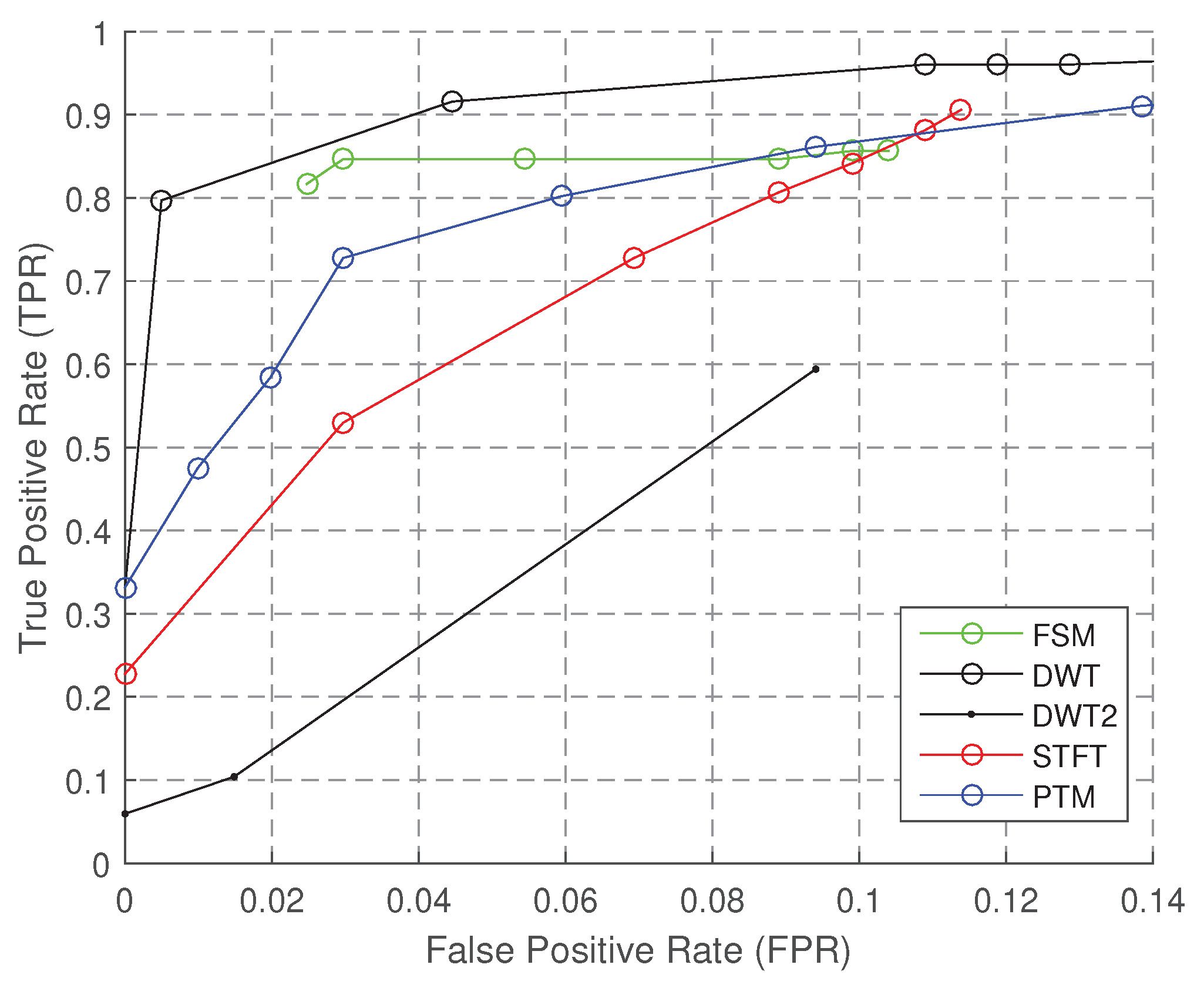
| PTM | STFT | FSM | DWT | DWT2 | |
|---|---|---|---|---|---|
| TPR | 91.0% | 97.2% | 95.7% | 98.1% | 80.0% |
| FPR | 0.3% | 0.52% | 0.1% | 0.3% | 0.3% |
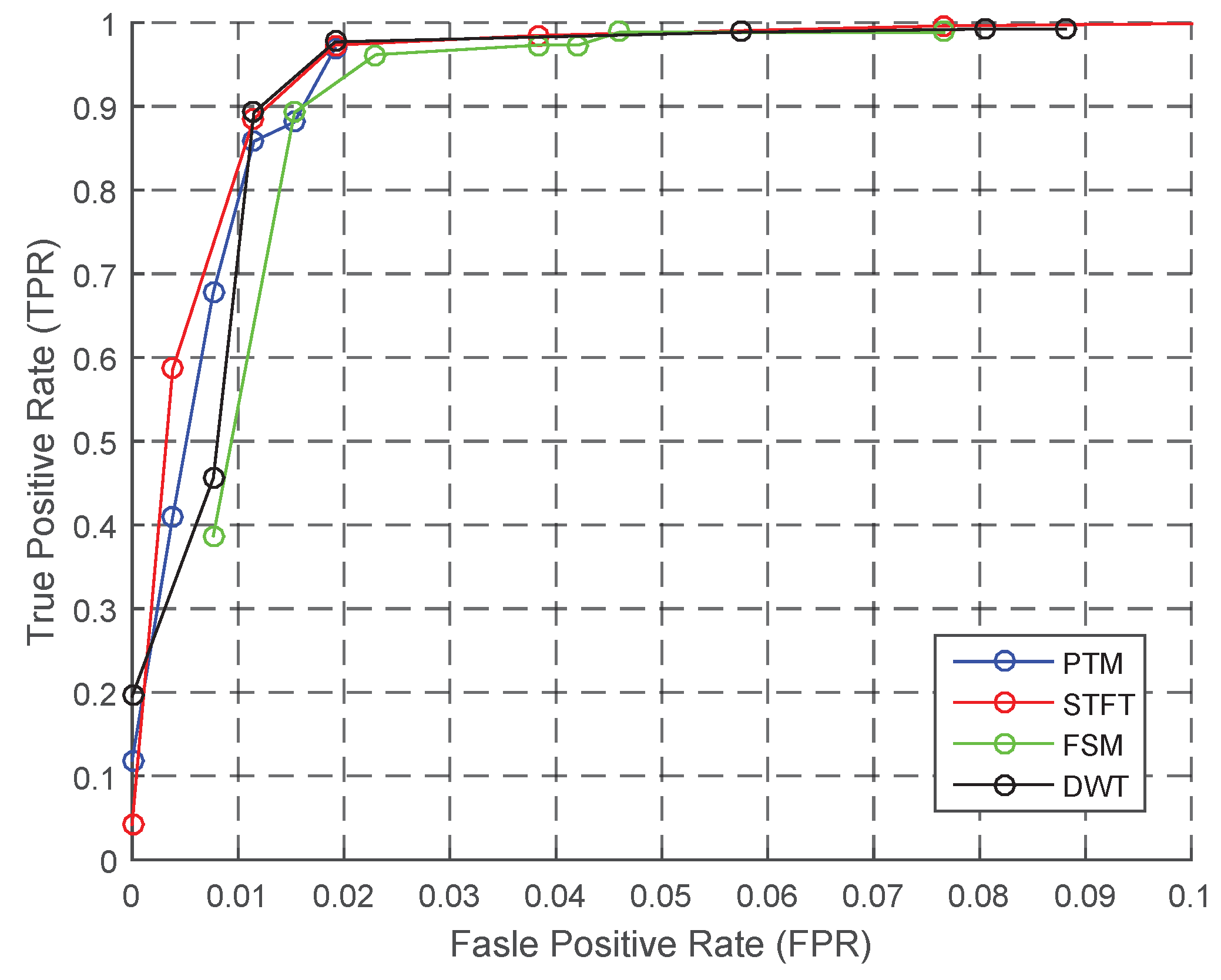
| PTM | STFT | FSM | DWT | DWT2 | |
|---|---|---|---|---|---|
| TPR | 98.7% | 99.57% | 99.13% | 92.61% | 95.65% |
| FPR | 1.73% | 0% | 0% | 5.21% | 3.47% |
| Group | Algorithm | Orientation | Personalization | Placement (Hand, Foot, etc.) | Sampling Rate (5 Hz to 200 Hz) |
|---|---|---|---|---|---|
| Heuristic Method | FSM | +1.5% | +9% | [−5%, +10%] | [−32%, +0%] |
| Signal Processing | PTM | +1% | +16% | [−49%, +17%] | [−28%, +0%] |
| STFT | +3% | +5% | [−46%, +9%] | [−25%, +0%] | |
| DWT | +1% | −1% | [−8%, +28%] | [−30%, +0%] | |
| DWT2 | −11% | +11% | [−42%, +31%] | [−40%, +0%] |
| Group | Algorithm | Orientation | Personalization | Placement (Hand, Foot, etc.) | Window Size (1.5 s to 6 s) | Sampling Rate (5 Hz to 200 Hz) |
|---|---|---|---|---|---|---|
| Heuristic Method | THR | −0.3% | +9% | [−3%, +8%] | [−2%, +5%] | [−1%, +1%] |
| Signal Processing | STFT | −8% | +13% | [−15%, +15%] | [−16%, +1%] | [−13%, +1%] |
| DWT | +1% | +10% | [−8%, +9%] | [−5%, +4%] | [−12%, +1%] | |
| Machine Learning | k-NN | +10% | +15% | [−1%, +10%] | [−6%, +7%] | [−12%, +3%] |
| SVM | +8% | +11% | [−8%, +7%] | [−2%, +2%] | [−12%, +2%] |
© 2018 by the authors. Licensee MDPI, Basel, Switzerland. This article is an open access article distributed under the terms and conditions of the Creative Commons Attribution (CC BY) license (http://creativecommons.org/licenses/by/4.0/).
Share and Cite
Ao, B.; Wang, Y.; Liu, H.; Li, D.; Song, L.; Li, J. Context Impacts in Accelerometer-Based Walk Detection and Step Counting. Sensors 2018, 18, 3604. https://doi.org/10.3390/s18113604
Ao B, Wang Y, Liu H, Li D, Song L, Li J. Context Impacts in Accelerometer-Based Walk Detection and Step Counting. Sensors. 2018; 18(11):3604. https://doi.org/10.3390/s18113604
Chicago/Turabian StyleAo, Buke, Yongcai Wang, Hongnan Liu, Deying Li, Lei Song, and Jianqiang Li. 2018. "Context Impacts in Accelerometer-Based Walk Detection and Step Counting" Sensors 18, no. 11: 3604. https://doi.org/10.3390/s18113604
APA StyleAo, B., Wang, Y., Liu, H., Li, D., Song, L., & Li, J. (2018). Context Impacts in Accelerometer-Based Walk Detection and Step Counting. Sensors, 18(11), 3604. https://doi.org/10.3390/s18113604