Multi-Target Detection Method Based on Variable Carrier Frequency Chirp Sequence

Abstract
:1. Introduction
- (1)
- Waveforms must have probing capabilities for multi-target scenes to meet the application requirements of intelligent transportation, automotive collision detection, etc.
- (2)
- Under current conditions, it is difficult to meet the accuracy requirements by extracting the phase information to solve the parameters such as velocity and range. Waveforms must be simple in form and easy to implement in hardware.
- (3)
- It is not possible to increase the computational complexity and increase the cost of hardware because of the special signal form.
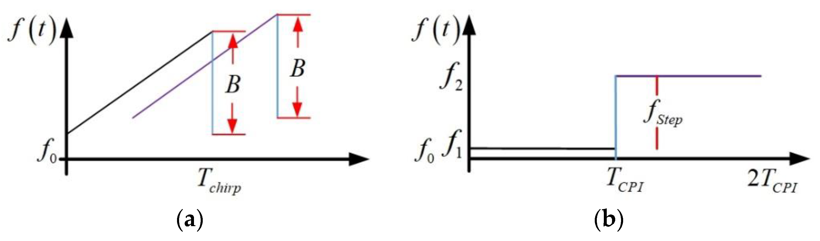
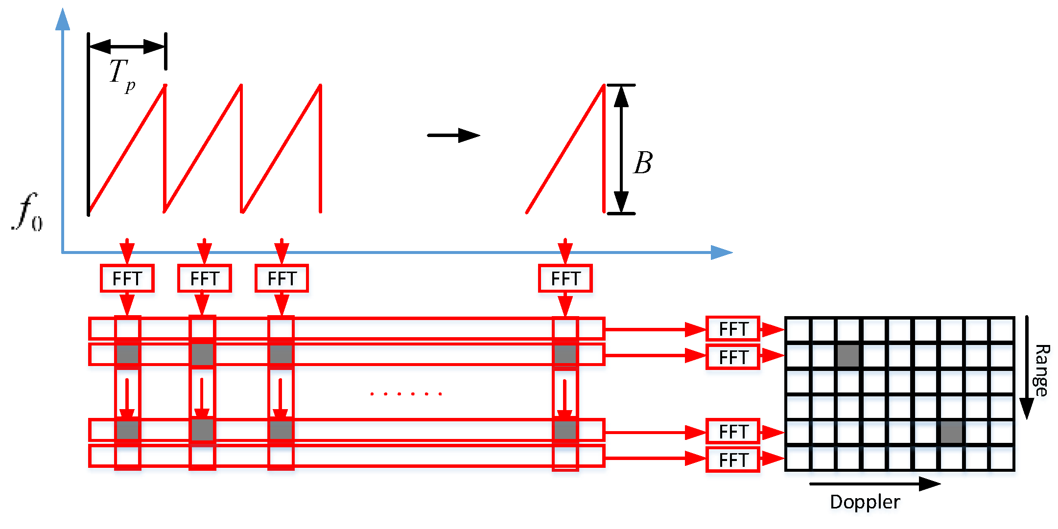
2. Chirp Sequence Waveform
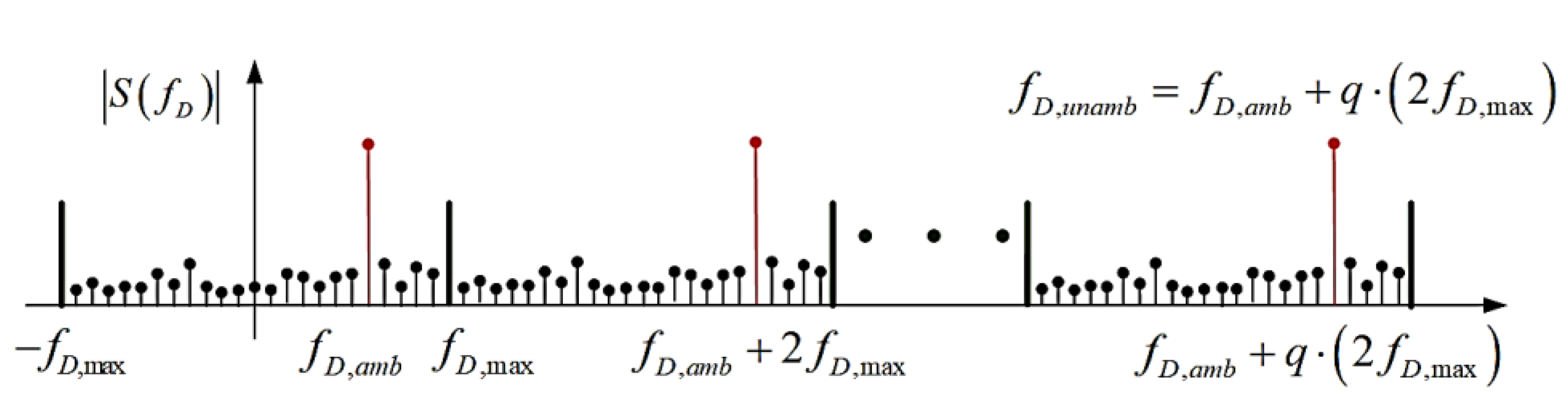
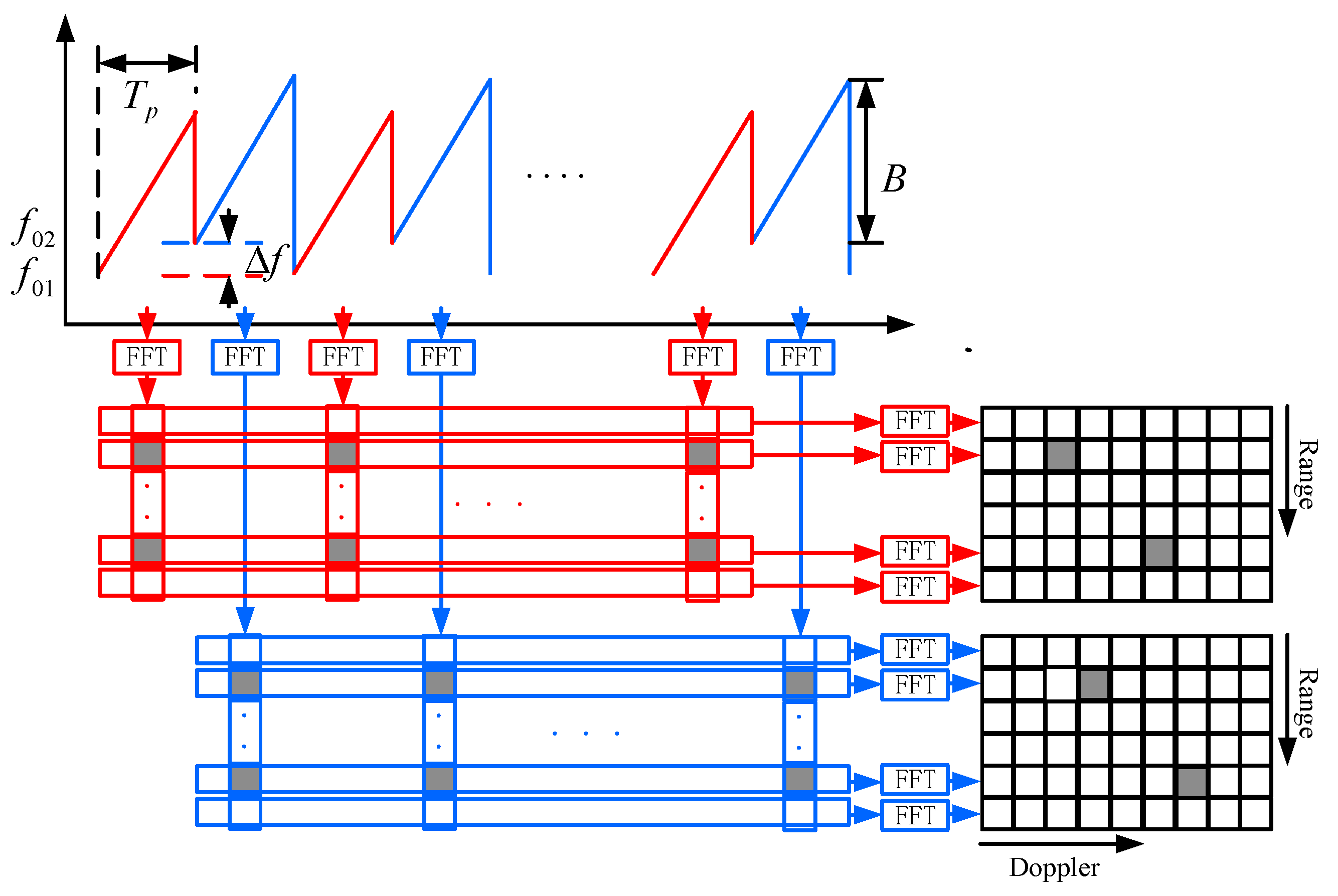
3. Variable Carrier Frequency Chirp Sequence
4. Simulation
5. Conclusions
Author Contributions
Funding
Conflicts of Interest
References
- Han, L.; Wu, K. Radar and radio data fusion platform for future intelligent transportation system. In Proceedings of the 7th European Radar Conference, Paris, France, 30 September–1 October 2010; pp. 65–68. [Google Scholar]
- Kandar, D.; Sur, S.N.; Bhaskar, D.; Guchhait, A.; Bera, R.; Sarkar, C.K. An approach to converge communication and radar technologies for intelligent transportation system. Indian J. Sci. Technol. 2010, 3, 417–421. [Google Scholar]
- Bloecher, H.L.; Dickmann, J.; Andres, M. Automotive active safety & comfort functions using radar. In Proceedings of the 2009 IEEE International Conference on Ultra-Wideband, Vancouver, BC, Canada, 9–11 September 2009; pp. 490–494. [Google Scholar]
- Hasch, J.; Topak, E.; Schnabel, R.; Zwick, T.; Weigel, R.; Waldschmidt, C. Millimeter-wave technology for automotive radar sensors in the 77 GHz frequency band. IEEE Trans. Microw. Theory Tech. 2012, 60, 845–860. [Google Scholar] [CrossRef]
- Damien, V.; Paul, C.; Roland, C. Localization and Mapping Using Only a Rotating FMCW Radar Sensor. Sensors 2013, 13, 4527–4552. [Google Scholar] [CrossRef] [Green Version]
- Li, C.; Chen, W.; Liu, G.; Yan, R.; Xu, H.; Qi, Y. A noncontact FMCW radar sensor for displacement measurement in structural health monitoring. Sensors 2015, 15, 7412–7433. [Google Scholar] [CrossRef] [PubMed]
- Wang, T.; Zheng, N.; Xin, J.; Ma, Z. Integrating millimeter wave radar with a monocular vision sensor for on-road obstacle detection applications. Sensors 2011, 11, 8992–9008. [Google Scholar] [CrossRef] [PubMed]
- Hyun, E.; Jin, Y.-S.; Lee, J.-H. A pedestrian detection scheme using a coherent phase difference method based on 2D range-doppler FMCW radar. Sensors 2016, 16, 124. [Google Scholar] [CrossRef] [PubMed]
- Fölster, F.; Rohling, H. Signal processing structure for automotive radar. Frequenz 2006, 60, 20–24. [Google Scholar] [CrossRef]
- Rohling, H. Milestones in radar and the success story of automotive radar systems. In Proceedings of the International Radar Symposium, Vilnius, Lithuania, 16–18 June 2010; pp. 1–6. [Google Scholar]
- Chadwick, R.B.; Straucih, R.G. Processing of FM-CW Doppler Radar Signals from Distributed Targets. IEEE Trans. Aerosp. Electron. Syst. 1979, AES-15, 185–189. [Google Scholar] [CrossRef]
- Rohling, H.; Meinecke, M.-M.; Klotz, M.; Mende, R. Experiences with an experimental car controlled by a 77 GHz radar sensor. In Proceedings of the International Radar Symposium, Munich, Germany, 15–17 September 1998; pp. 345–354. [Google Scholar]
- Kuroda, H.; Nakamura, M.; Takano, K.; Kondoh, H. Fully-MMIC 76 GHz radar for ACC. In Proceedings of the 2000 IEEE Intelligent Transportation Systems (ITSC2000), Proceedings (Cat. No.00TH8493), Dearborn, MI, USA, 1–3 October 2000; pp. 299–304. [Google Scholar]
- Marc-Michael, M. Combination of LFCM and FSK Modulation Principles for Automotive Radar Systems. In Proceedings of the German Radar Symposium (GSR2000), Berlin, Germany, 11–12 October 2000. [Google Scholar]
- Rohling, H.; Meinecke, M.M. Waveform design principles for automotive radar systems. In Proceedings of the 2001 CIE International Conference on Radar Proceedings (Cat No. 01TH8559), Beijing, China, 15–18 October 2001; pp. 1–4. [Google Scholar]
- He, J.; Zhang, R.; Sheng, W.; Han, Y.; Ma, X. An improved MFSK waveform for low-cost automotive radar. In Proceedings of the 2016 CIE International Conference on Radar (RADAR), Guangzhou, China, 10–13 October 2016; pp. 1–5. [Google Scholar]
- Nguyen, Q.; Park, M.; Kim, Y.; Bien, F. 77 GHz waveform generator with multiple frequency shift keying modulation for multi-target detection automotive radar applications. Electron. Lett. 2015, 51, 595–596. [Google Scholar] [CrossRef]
- Stove, A.G. Linear FMCW radar techniques. IEE Proc. F 1992, 139, 343–350. [Google Scholar] [CrossRef]
- Kim, G.; Mun, J.; Lee, J. A Peer-to-peer Interference Analysis for Automotive Chirp Sequence Radars. IEEE Trans. Veh. Technol. 2018, 67, 8110–8117. [Google Scholar] [CrossRef]
- Pourvoyeur, K.; Feger, R.; Schuster, S.; Stelzer, A.; Maurer, L. Ramp sequence analysis to resolve multi target scenarios for a 77-GHz FMCW radar sensor. In Proceedings of the 2008 11th International Conference on Information Fusion, Cologne, Germany, 30 June–3 July 2008; pp. 1–7. [Google Scholar]
- Thurn, K.; Shmakov, D.; Li, G.; Max, S.; Meinecke, M.M.; Vossiek, M. A novel interlaced chirp sequence radar concept with range-Doppler processing for automotive applications. In Proceedings of the 2015 IEEE MTT-S International Microwave Symposium, Phoenix, AZ, USA, 17–22 May 2015; pp. 1–4. [Google Scholar]
- Kronauge, M.; Schroeder, C.; Rohling, H. Radar target detection and Doppler ambiguity resolution. In Proceedings of the 11th International Radar Symposium, Vilnius, Lithuania, 16–18 June 2010; pp. 1–4. [Google Scholar]
- Rohling, H.; Kronauge, M. New radar waveform based on a chirp sequence. In Proceedings of the 2014 International Radar Conference, Lille, France, 13–17 October 2014; pp. 1–4. [Google Scholar]
- Kronauge, M.; Rohling, H. New chirp sequence radar waveform. IEEE Trans. Aerosp. Electron. Syst. 2014, 50, 2870–2877. [Google Scholar] [CrossRef]
- Kronauge, M.; Rohling, H. Fast Two-Dimensional CFAR Procedure. IEEE Trans. Aerosp. Electron. Syst. 2013, 49, 1817–1823. [Google Scholar] [CrossRef]
- Wang, Y.; Xiao, Z.; Wu, L.; Xu, J.; Zhao, H. Jittered Chirp Sequence Waveform in combination with CS-based unambiguous doppler processing for automotive FMCW radar. IET Radar Sonar Navig. 2017, 11, 1877–1885. [Google Scholar] [CrossRef]


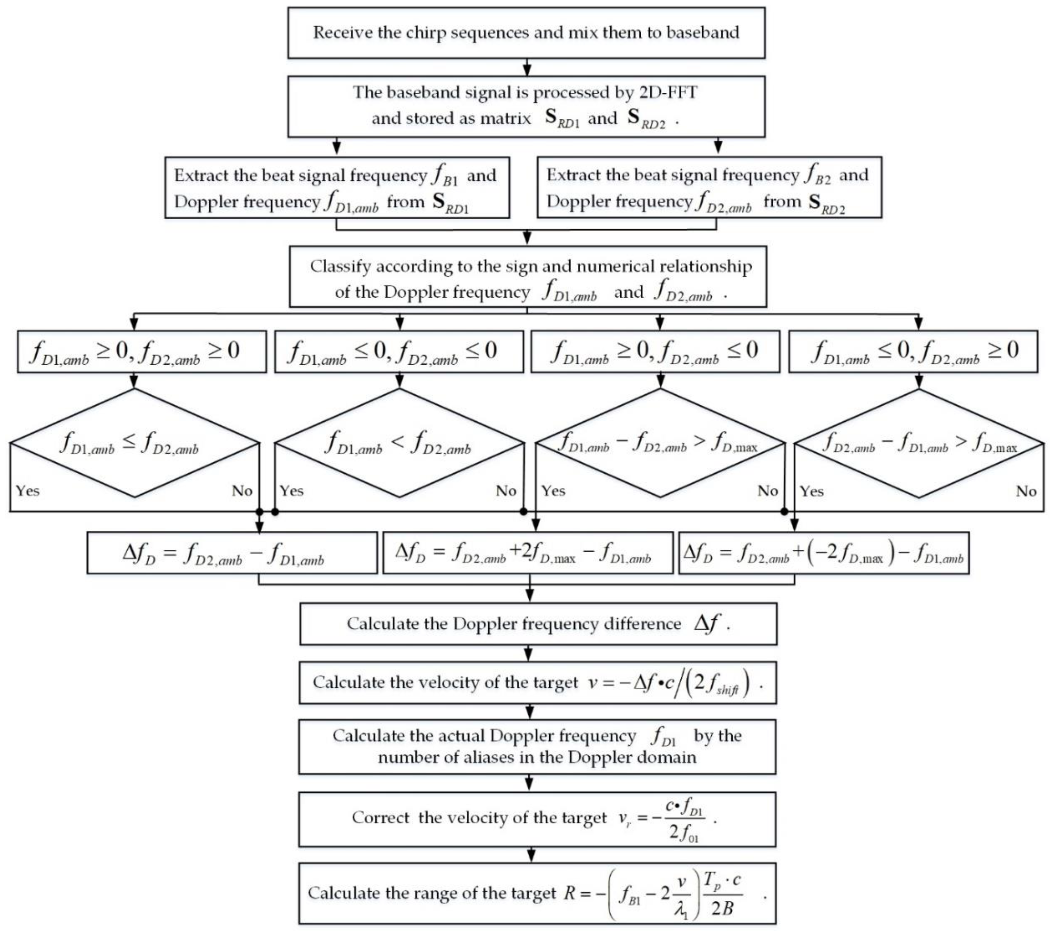
| Sign | Numerical Relationship | Doppler Frequency Difference | Velocity | Case |
|---|---|---|---|---|
| , | 1 | |||
| , | 2 | |||
| , | 3 | |||
| , | 4 | |||
| , | 5 | |||
| , | 6 | |||
| , | 7 | |||
| , | 8 |
| Parameters | Symbol |
|---|---|
| The First Carrier Frequency | |
| The Second Carrier Frequency | |
| Sweep Bandwidth | |
| The Chirp Duration | |
| Chirp Cycles | |
| FFT Length for Range Domain | |
| FFT Length for Doppler Domain |
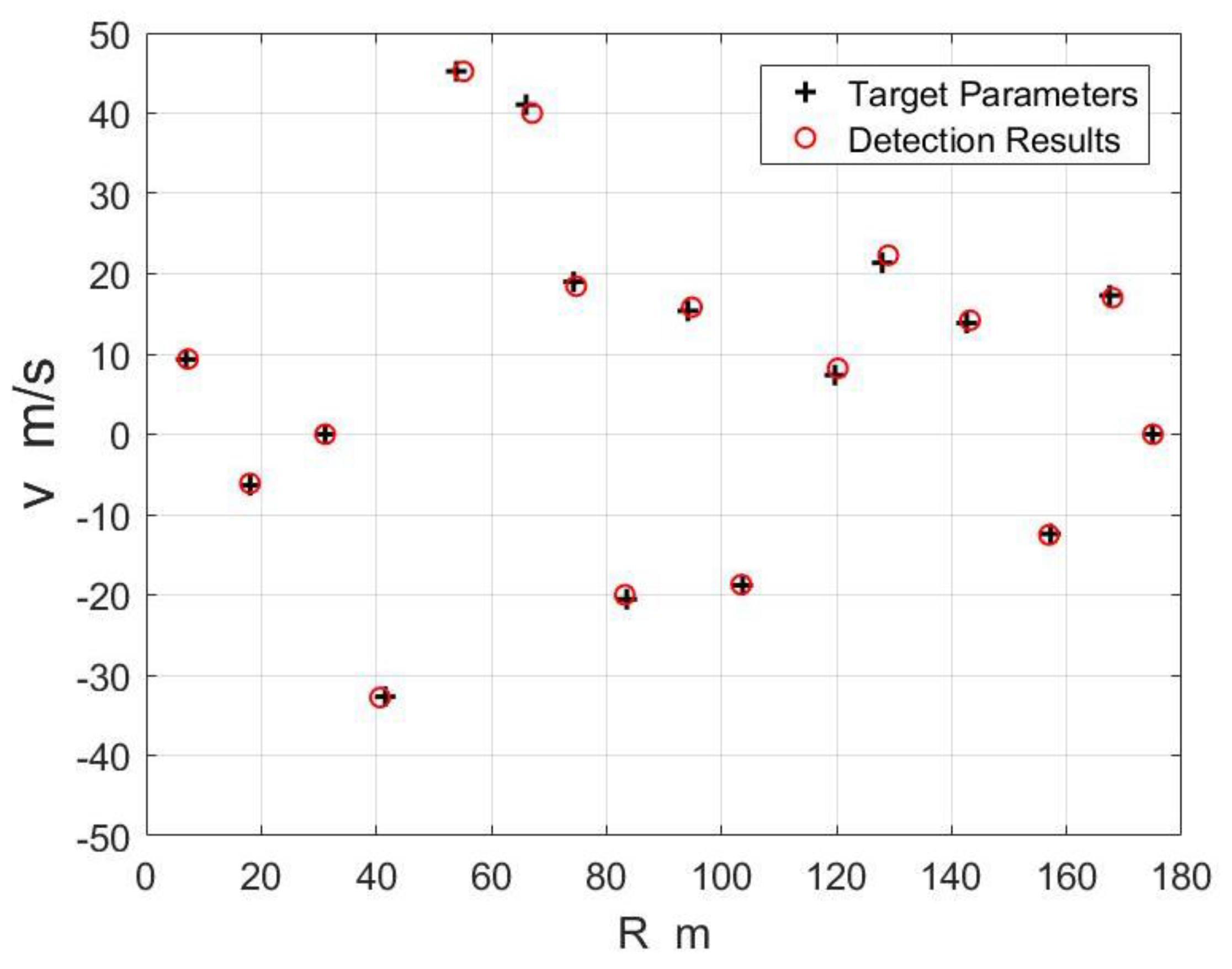
| Simulation Parameters | Measurement Results | Case | |||||
|---|---|---|---|---|---|---|---|
| m | m/s | m | m/s | ||||
| 7.27 | 9.37 | 3.66 | −5.62 | −9.28 | 6.94 | 9.34 | 6 |
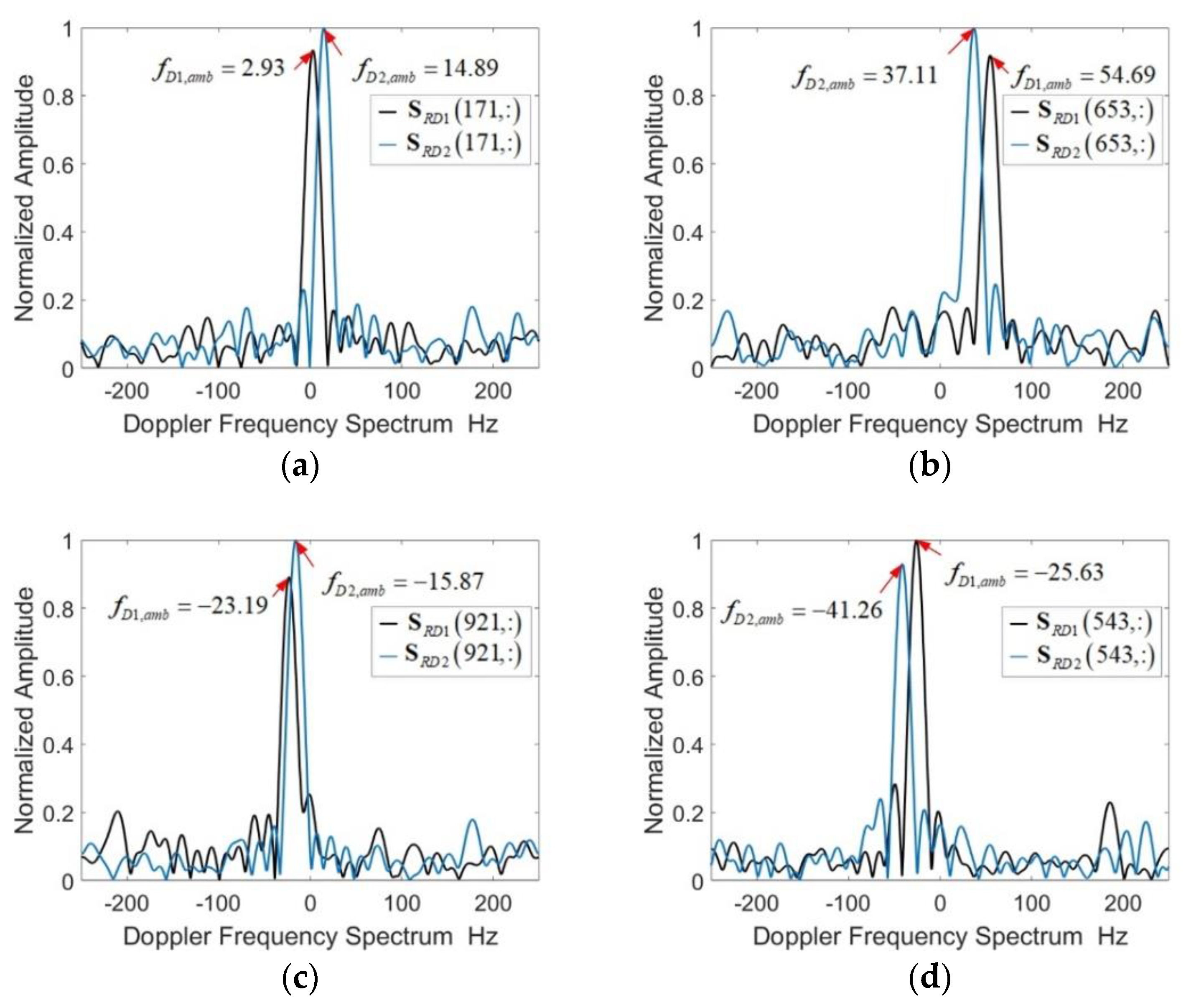
| 18.05 | −6.12 | −23.19 | −15.87 | 7.32 | 18.06 | −6.35 | 3 |
| 31.13 | 0.00 | 0.73 | 0.24 | −0.49 | 31.24 | 0.00 | 2 |
| 40.65 | −32.79 | 235.60 | −231.69 | 32.71 | 41.53 | −32.70 | 5 |
| 55.15 | 45.21 | −218.26 | 236.08 | −45.66 | 53.92 | 45.23 | 7 |
| 67.10 | 40.00 | 113.77 | 71.29 | −42.48 | 66.38 | 41.08 | 2 |
| 74.75 | 18.45 | 54.69 | 37.11 | −17.58 | 74.32 | 18.98 | 2 |
| 83.20 | −20.00 | 192.63 | 213.62 | 20.99 | 83.45 | −20.54 | 1 |
| 94.86 | 15.82 | −25.63 | −41.26 | −15.63 | 94.17 | 15.37 | 4 |
| 103.44 | −18.72 | −10.74 | 8.54 | 19.28 | 103.69 | −18.82 | 8 |
| 120.23 | 8.22 | 187.26 | 179.20 | −8.06 | 119.88 | 7.37 | 2 |
| 129.00 | 22.30 | −61.28 | −83.74 | −22.46 | 128.22 | 21.36 | 4 |
| 143.22 | 14.20 | 233.15 | 218.51 | −14.64 | 142.84 | 13.87 | 2 |
| 156.92 | −12.54 | 2.93 | 14.89 | 11.96 | 157.23 | −12.41 | 1 |
| 168.00 | 17.00 | −213.62 | −231.69 | 18.07 | 167.49 | 17.30 | 4 |
| 175.00 | 0.00 | 0.24 | 0.24 | 0.00 | 174.94 | 0.00 | 1 |
© 2018 by the authors. Licensee MDPI, Basel, Switzerland. This article is an open access article distributed under the terms and conditions of the Creative Commons Attribution (CC BY) license (http://creativecommons.org/licenses/by/4.0/).
Share and Cite
Wang, W.; Du, J.; Gao, J. Multi-Target Detection Method Based on Variable Carrier Frequency Chirp Sequence. Sensors 2018, 18, 3386. https://doi.org/10.3390/s18103386
Wang W, Du J, Gao J. Multi-Target Detection Method Based on Variable Carrier Frequency Chirp Sequence. Sensors. 2018; 18(10):3386. https://doi.org/10.3390/s18103386
Chicago/Turabian StyleWang, Wei, Jinsong Du, and Jie Gao. 2018. "Multi-Target Detection Method Based on Variable Carrier Frequency Chirp Sequence" Sensors 18, no. 10: 3386. https://doi.org/10.3390/s18103386
APA StyleWang, W., Du, J., & Gao, J. (2018). Multi-Target Detection Method Based on Variable Carrier Frequency Chirp Sequence. Sensors, 18(10), 3386. https://doi.org/10.3390/s18103386