Calibrating the Severity of Forest Defoliation by Pine Processionary Moth with Landsat and UAV Imagery


1
Centre for Ecological Research and Forestry Applications (CREAF), 08193 Cerdanyola del Vallès, Spain
2
InForest JRU (CTFC-CREAF), 25280 Solsona, Spain
3
Spanish National Research Council (CSIC), 08193 Cerdanyola del Vallès, Spain
*
Authors to whom correspondence should be addressed.
Sensors 2018, 18(10), 3278; https://doi.org/10.3390/s18103278
Submission received: 22 August 2018
/
Revised: 18 September 2018
/
Accepted: 26 September 2018
/
Published: 29 September 2018
(This article belongs to the Special Issue Remote Sensing and Its Applications in the Bio-Geosciences)
Abstract
:The pine processionary moth (Thaumetopoea pityocampa Dennis and Schiff.), one of the major defoliating insects in Mediterranean forests, has become an increasing threat to the forest health of the region over the past two decades. After a recent outbreak of T. pityocampa in Catalonia, Spain, we attempted to estimate the damage severity by capturing the maximum defoliation period over winter between pre-outbreak and post-outbreak images. The difference in vegetation index (dVI) derived from Landsat 8 was used as the change detection indicator and was further calibrated with Unmanned Aerial Vehicle (UAV) imagery. Regression models between predicted dVIs and observed defoliation degrees by UAV were compared among five selected dVIs for the coefficient of determination. Our results found the highest R-squared value (0.815) using Moisture Stress Index (MSI), with an overall accuracy of 72%, as a promising approach for estimating the severity of defoliation in affected areas where ground-truth data is limited. We concluded with the high potential of using UAVs as an alternative method to obtain ground-truth data for cost-effectively monitoring forest health. In future studies, combining UAV images with satellite data may be considered to validate model predictions of the forest condition for developing ecosystem service tools.
1. Introduction
Currently, pest insects are the principal biotic drivers causing disturbances threatening Mediterranean forests in combination with abiotic factors such as drought, fire and climate change [1,2]. The pine processionary moth (Thaumetopoea pityocampa Dennis and Schiff.), one of the major defoliating insects in Mediterranean pine forests, has been considered by the Intergovernmental Panel on Climate Change (IPCC) as an indicator of global warming [3] for being recorded in an expanded biogeographical range of host distribution from Southern Europe in the Mediterranean region towards northern latitudes and higher elevations over the past twenty years [4,5]. Consequently, the defoliators may continue to increase with the future trend of climate change scenarios [5].
Outbreaks of T. pityocampa have been observed to be cycles of 6 years on average [2,6], mainly in managed young stands [5,7]. In a normal year healthy forest stands recover from defoliation, however, periodic outbreaks attack large forests in which host trees may suffer up to 100% defoliation. Thus, severely affected stands may result in significant reductions of individual tree growth, stand productivity, and forest ecosystem health, from tree to stand and landscape levels [5,8]. Such growth reduction may accelerate the rate of tree mortality when the damage is accumulated due to other biotic factors as well as abiotic factors [9]. As a consequence, defoliation focused on host pine trees is more likely to change the structure and species composition in natural stands as well as lose economic values in planted stands [2,9]. Furthermore, forest ecosystems at the landscape level are major carbon sinks contributing to mitigate the impacts of climate change [10,11,12]. Therefore, to predict future scenarios on forest productivity and mortality in cases where the outbreaks may occur, reliable data from monitoring the pest distribution at regional and national scales are required [5,12].
Despite the annual ground survey on forest health in the Mediterranean countries such as France, Portugal and Spain which are frequently affected by outbreaks of T. pityocampa, we currently lack accurate, fine-grained and timely information systems for monitoring the latest forest condition. Thus, an efficient tool to improve such regional or national monitoring systems spatially and temporally may be developed by adequately using the latest remote sensing technologies. In addition to conventional field surveys which are often time-consuming to cover large areas, satellite-based images such as MODIS and Landsat at medium spatial resolution (30–250 m) have been widely used for detecting defoliations in forest systems over the past two decades [1]. Currently, due to the free accessibility to medium-resolution (10–60 m) products from Landsat 8 [13] and Sentinel-2 [14], they are most commonly used for cost-effectively monitoring large areas. For sensors at high spatial resolution (<10 m), the private industry continued to launch satellites such as IKONOS, QuickBird, RapidEye and TerraSAR-X [1]. With further advancements in spaceborne technology, the sensor’s spatial resolution nowadays can be as high as 0.3 m (WorldView-4), and continue to enhance temporal and spectral resolution as well [15]. In Spain, using various sensors (Airborne Hyperspectral Scanner, Hyperion, ChrisProba, Quickbird, and Landsat), Cabello et al. [16] have applied vegetation indices for mapping forest damage caused by T. pityocampa to estimate the Leaf Area Index in affected pine stands, followed by Sangüesa-Barreda et al. [2] with the combined method of Landsat-derived vegetation indices and dendrochronology for assessing the tree growth reduction affected by outbreaks of T. pityocampa. Furthermore, the emergence of airborne laser scanning (ALS) characterized by point clouds complements the three-dimensional (3D) structure in addition to the spatial resolution higher than any spaceborne technology [1,17]. Using ALS metrics, classification of defoliated Scots pines at the individual tree level was demonstrated by Kantola et al. [18].
Since the cost of above high-resolution products remains a limiting factor for small operational areas, the trend of monitoring forest health in recent studies has shifted to the alternative 3D technology based on cost-effective Unmanned Aerial Vehicle (UAV) at high temporal and spatial resolution over the past decade [19]. While initial studies with UAVs were focused on crop management for agriculture applications, the latest UAV technology has proved to be effective for forestry applications (forest disturbances and diseases, forest cover mapping, tree species identification, and forest inventory measurements) as a sampling tool for acquiring ground-truth data [20]. To date only a few studies have examined on the classification accuracy of forest insect defoliations using UAV imagery. The classification methods include Random Forest [19], object-based image analysis (OBIA) [21,22], k-Nearest Neighbor [23], and maximum likelihood [24,25]. Moreover, no study has calibrated satellite-based vegetation indices as a predictive indicator of such defoliation with UAV-derived data as ground-truth while Pla et al. [26] has recently made progress in calibrating some indices specific to fire damage using UAV imagery.
With the objective to quantify forest response to infestation, we developed remote sensing-derived indicators to measure the defoliation levels. In this study, we aim to evaluate the spatiotemporal degree of defoliation during a recent outbreak of T. pityocampa in Mediterranean pine forests by change detection analysis using a combination of satellite and UAV imagery. Our main objectives are: (1) examine regression models between vegetation indices (VI) derived from Landsat imagery and defoliation degrees interpreted by UAV imagery for calibration; (2) map defoliation classes based on the best-fit VI model to assess classification accuracy for validation.
2. Materials and Methods
2.1. Study Area
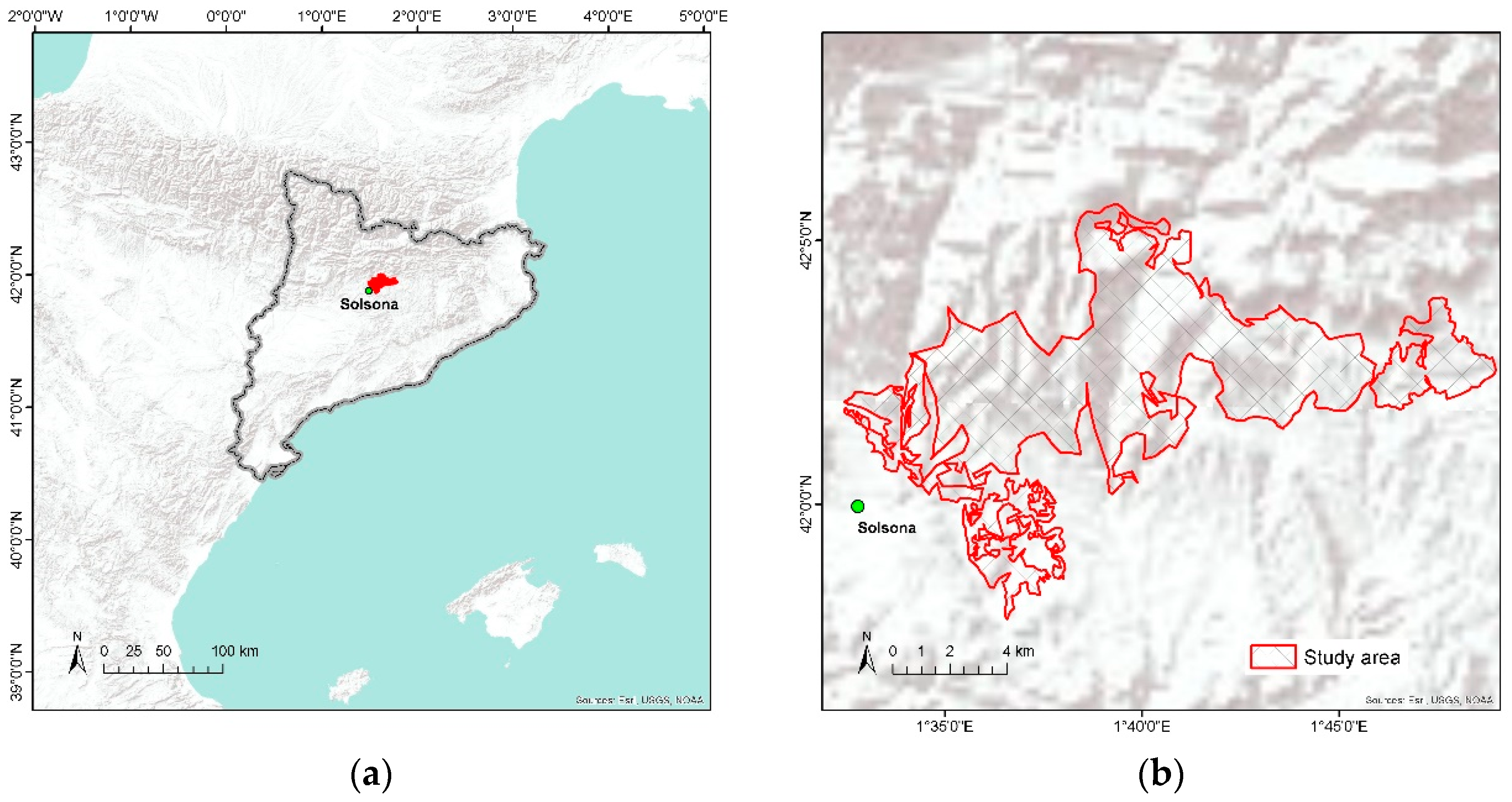
The study area is located near the city of Solsona, Catalonia, northeast of Spain (Figure 1a), encompassing 6809 hectares (Figure 1b) dominated by pine forests (elevation above sea level ranging from 600 m to 1100 m). Primary host species are Pinus nigra followed by P. sylvestris, which are the dominant tree species in mixed stands with Quercus ilex and Q. humilis. The climate is Mediterranean continental characterized by hot summer and cold winter. According to the local meteorological station, the mean annual temperature is 11.7 °C and the mean total annual precipitation is 864 mm. As larvae of T. pityocampa develop across winter, it has benefited from recent warmer fall and winter temperatures for overcoming the thermal thresholds and consequently increasing the rate of larval survival and growth as far as the host trees are present [5].
2.2. Field Data
Ground and aerial sketch mapping data were first obtained from the regional forest health inventory during the years from 2010 to 2016. Since the project on evaluating the severity of infestations caused by T. pityocampa started, field surveys have been conducted by rural agents every winter when the symptoms are visually most evident from February to March after the larvae complete feeding on needles and go into the soil for pupation [4]. The survey form is standardized by the government (Generalitat de Catalunya) and filled out by rural agents. Affected stands are mapped as polygons, on average about 137 hectares per polygon ranging to the smallest of 0.03 hectare, with attributes such as observation date, forest type, aspect, tree species, and infestation severity. The severity scales are ranked from 1 to 4 at highest as follows: (1) several nests at the margins and some nests in the center of the forest stand; (2) partial defoliation at the margins on some trees and several nests in the center of the forest stand; (3) intense defoliation at the margins and partial defoliation in the forest stand; (4) very intense defoliation both at the margins and in the center of the forest stand. The total area infested by T. pityocampa was recorded at largest in 2016. Based on this inventory database with sketch map polygons, our study area was selected to be one of the most severely affected areas during winter 2015–2016 (Figure 1b).
2.3. Landsat Images and Vegetation Indices
Pre-outbreak (20 September 2015) and post-outbreak (30 March 2016) images were obtained from Landsat 8 (path 198, row 31) with minimum clouds to capture the maximum defoliation period from fall to spring. Surface Reflectance (SR) products were downloaded from the GloVis (http://glovis.usgs.gov) USGS server. Furthermore, the Band Quality Assessment included in the SR product was applied to exclude pixels described as water, snow, cloud, and cloud shadow so that only pixels with values indicating clear terrain were extracted [2,26,27]. Preprocessed images in the cartographic UTM projection were further extracted by forest cover classified as pine-dominated stands according to the Land Cover Map of Catalonia (MCSC) generated in 2009. The best spectral regions for defoliation detection may correspond to reflectance bands from Landsat 8 such as near infrared (NIR = Band 5) and shortwave infrared (SWIR1 = Band 6 and SWIR2 = Band 7) which enable to capture a fast reduction of pine foliage and the consequent reduction in tree evapotranspiration [1,26]. In this study, we tested five VIs to predict the defoliation degree in pine forests as summarized in Table 1.
Comparing values of VI among multiple dates may function as a good indicator for change detection [1,4,16,17,18]. To distinguish annual defoliation during the outbreak from cumulative defoliation over several years, a pre-outbreak (20 September 2015) image was compared to additional images from Landsat 8 representing the month of September in the previous two years (2013 and 2014) to confirm that there was no abrupt change in the VI values used in our study area before outbreak. The difference in VI (dVI) was calculated by simply subtracting the value of each VI in year 2016 (post-outbreak) from year 2015 (pre-outbreak) to estimate annual defoliation:
VI (pre-outbreak) − VI (post-outbreak) = dVI
2.4. Visual Interpretation with UAV Images
To assess the level of defoliation in selected locations, we used a camera (FC200, DJI, Shenzhen, China) mounted on a UAV (Phantom 2 vision+, DJI, Shenzhen, China). This camera can capture images, photos or videos, in the visible spectrum (RGB including blue, green and red bands) with a lens focal length of 5 mm and field of view of 120 degrees [33]. The RGB imagery had a 14 megapixels-resolution and was collected from a flying altitude ranging at 50–100 m above the ground level, resulting in a ground sample distance (GSD) of 2.0–3.5 cm. Seven flight surveys were conducted between December 2015 and March 2016 covering approximately 193 hectares across the study area shown in Figure 2a, of which five were collected in photos (81 hectares) and two were recorded in videos (112 hectares) at speeds ranging from 4–8 m per second depending on light conditions. The survey locations were selected to represent the stand types characterized by P. nigra and P. sylvestris and by various defoliation levels. Some surveys were recorded earlier than the post-outbreak image (30 March 2016) where high defoliation levels had been already observed at that time.
The total of 526 adjacent photos overlapped (forward 80%, side 60%) from the five flights with their geotagged locations were processed in the software PhotoScan Professional 1.4.0 (Agisoft LLC, St. Petersburg, Russia). In the image processing they were geometrically aligned to build a point cloud, 3D model, digital elevation model (DEM), and finally five orthomosaic images [34]. To collect more sample images, we included additional two videos flying at 4 m per second and recording 29 frames per second with the associated GPS files, which were imported into the software Video GeoTagger (Remote GeoSystems, Fort Collins, CO, USA) to tag geolocations. Extracting a frame per second resulted in the total of 339 frames in photo files. We repeated the same image processing used for the photos to generate two additional orthomosaic images derived from the video frames.
Using the ArcGIS version 10.5 software (ESRI, Redlands, CA, USA) each orthomosaic was georeferenced to the Landsat imagery in the UTM projection by performing a first order polynomial transformation with 4 control points, obtaining an accuracy of sub-meter root mean square error. The georeferenced orthomosaic images were further stratified to delineate non-forested or forested areas with the severity of defoliation in homogenously affected stands by visual interpretation (Figure 2b).
As summarized in Table 2, the sampled grid cells of 30 m × 30 m on orthomosaic images, corresponding to the pixels captured by Landsat, were haphazardly selected by an analyst avoiding shadow pixels from each representative category. Upon delineating the surface area containing defoliated trees per grid cell, the defoliated portion of the total cell area (900 m2) was calculated and expressed at 5% interval (Figure 2c). Finally, all selected grid cells were classified into four categories: nil (no change = 0–5%); low (defoliation 10–30%); medium (defoliation 35–65%); and high (defoliation 70–100%), as a modified classification suggested by Hall et al. [35].
2.5. Regression Analysis and Threshold Classification
We statistically analyzed relationships between two variables, predicted dVI (X) from Landsat imagery and observed defoliation % (Y) from UAV imagery. The relationships between X and Y were evaluated using the software R in various regression models including simple linear, logarithmic, exponential, polynomial, and logistic models. Provided that the range of defoliation % (Y) is limited as the response variable is bounded from 0 to 1 [36,37,38], logistic regression was employed to express proportion defoliated, following the equation:
where X represents the value of pixel in a selected dVI within the sample image, Y represents the percentage of defoliation interpreted within an individual UAV sample image, and a and b are the slope and intercept of the regression function.
Based on fifty selected samples (sample size = 50) in the study area, regression models were fitted to evaluate the coefficient of determination, McFadden’s R2 [39], which is most often reported in statistical software and recommended for measures of fit for logistic regression [40]. The dVI models were then compared to determine the best-fit indicator for estimating the severity of defoliation. With the known Y values of 10, 35 and 70 to separate the range of defoliation %, threshold limits in dVI (X) from the Equation (2) were recalculated as follows:
2.6. Classification Accuracy
To assess an overall accuracy of the threshold classification, we generated a confusion matrix of the four defoliation classes in the 50 selected grid cells, which were compared between the Landsat-based prediction and UAV-based interpretation. Validation of classes in the severity map was performed by assessing classification accuracy of dVIs referenced to UAV observations.
3. Results
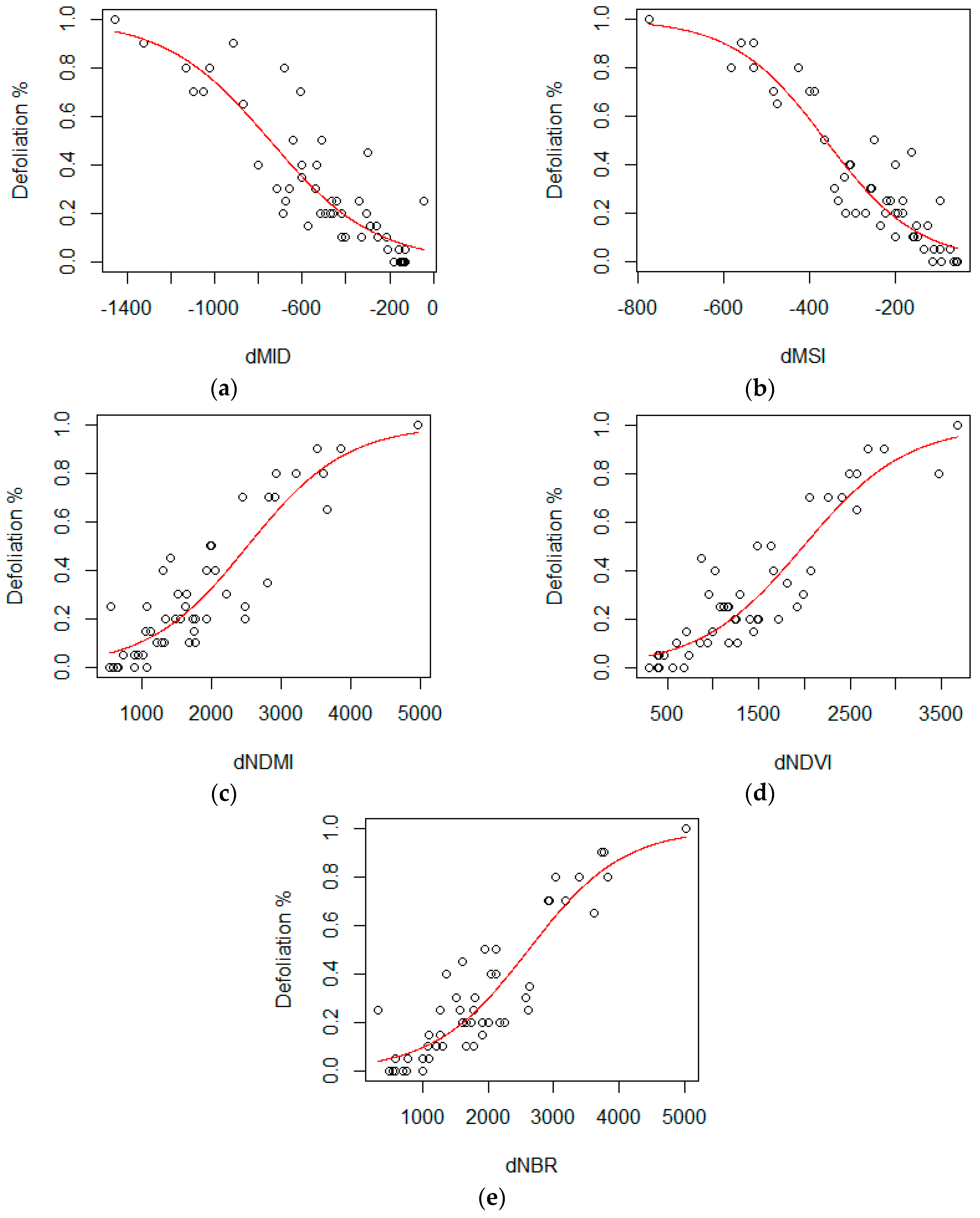
In Figure 3 the resulting X and Y points were plotted and compared among selected VIs. Moreover, the coefficient of determination (R2) by dVI is summarized in Table 3, which was statistically analyzed for logistic regression proposed by McFadden [39]. The goodness of fit was highest = 0.815 with dMSI while it was not improved by normalizing VIs such as dNDMI, dNDVI, and dNBR.
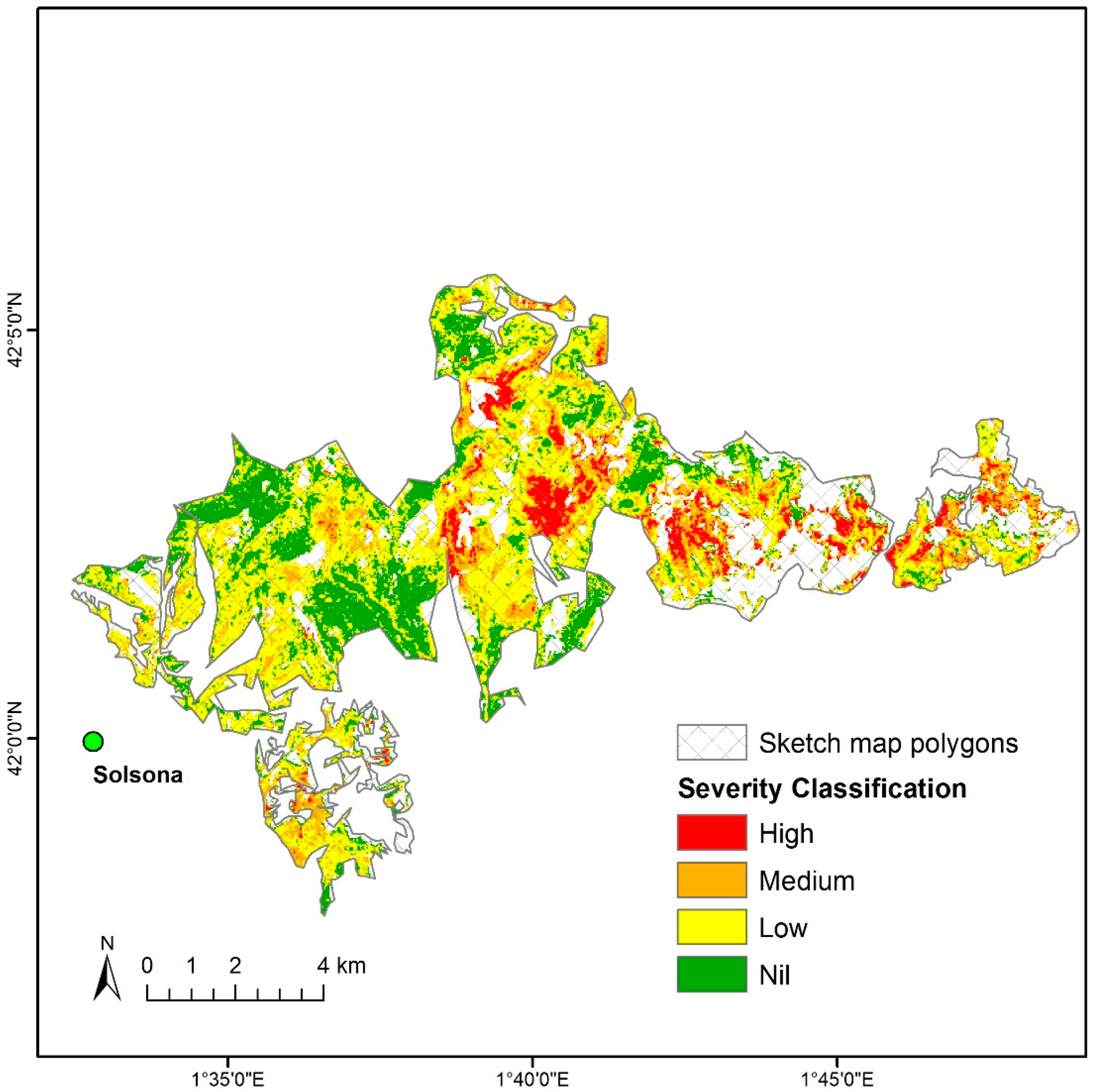
Using the equations in Table 3, the range of dVI values were determined as threshold limits in classification (Table 4). Applying values in dMSI to defoliation %, any value higher than −125 is classified as no defoliation (<10%): −125 to −295 (10–35%); −295 to −453 (35–70%); and lower than −453 (>70%). Based on the threshold limits, pixels assigned to four classes of defoliation were mapped to show the severity across the study area (Figure 4). The blank pixels in no color indicate either non-forested areas or stands dominated by other tree species, which were initially excluded from the analysis.
The overall accuracy of the threshold classification was presented in Table 5 for the four defoliation classes (nil, low, medium, and high) in the 50 selected samples of dMSI referenced to UAV orthomosaic images. Greatest producer’s accuracy representing a measure of omission error was 90% for the nil defoliation class, where nine out of the 10 cells observed as nil were correctly classified by predicted dMSI. On the other hand, the high defoliation class was mapped with greatest user’s accuracy of 86% indicating commission error, which six out the seven cells predicted as high correctly represented the observed class. Overall, it should be noted that the number of cells classified as nil or medium defoliation was overestimated whereas the one classified as low or high defoliation was underestimated. Finally, the overall accuracy of the classification was 72% calculated by the ratio between the sum of the cells correctly classified from each class and 50 cells in total.
4. Discussion
Among five VIs tested in our study, the results with dMSI as the best predictor were consistent with recent studies on insect defoliations [2,36,37,38]. The SWIR band calculated in dMSI is known to be a good indicator for the plant moisture content in addition to the plant stress detected in the NIR band [1,43]. It may be assumed that the MSI better indicated early symptoms of the host trees stressed by dehydration in our study. The first study examining MSI in relation to conifer damage was conducted by Vogelmann et al. [44], resulted with an R2 of 0.830 in linear regression. Other studies with MSI have been conducted in pine forests by Sangüesa-Barreda et al. [2] demonstrating the highest significance on ANOVA tests and most recently by Zhu et al. [38] with an R2 of 0.982 in logistic regression. The MSI was also effectively applied to defoliation in deciduous forests by Townsend et al. [36] with an R2 of 0.844 in logistic regression and Rullán-Silva et al. [37] with an R2 of 0.632 in sigmoidal mixed-effects models. For monitoring coniferous forests in general, the MSI has been found to be more effective than the NDVI which has been mainly applied to deciduous forests [38,43,44]. Nevertheless, several potentially robust VIs should be tested on each particular study area since tree-insect relationships vary from site to site [1].
Our initial attempt was to use sketch map polygons from field data as training samples for supervised classification on the severity of defoliation. However, the significant discrepancy in spatial resolution between the field data provided by regional rural agents and Landsat data became evident. The sketch map polygons were delineated for classifying severity levels at a coarse scale in hectares including non-forested areas whereas the spatial resolution of Landsat imagery is as fine as 30 m per pixel, which resulted in a wide range of values among pixels within the same polygon. Yet, without any ground observation such as nests of T. pityocampa, it is often difficult to distinguish the cause of defoliation based on only spectral bands or even aerial surveys at low levels of defoliation [8]. Further integration by training the rural agents to apply UAV workflows to their annual health survey may fill this monitoring gap. As suggested in the most recent review on forest health monitoring by Hall et al. [35], how spaceborne and airborne remote sensing may be integrated with aerial and field surveys into a multi-scale, multi-source monitoring system should be explored.
Regarding stand dynamics and species compositions, we extracted pine-dominated stands from the Land Cover Map of Catalonia (MCSC) and assumed that sampled stands were dense enough to represent Landsat VIs based on the defoliation degree of dominant species in pine stands. Nonetheless, we acknowledge the possibility of misrepresenting the VIs in severely defoliated stands to some extent where understory species is non-host evergreen such as Q. ilex which is not affected by T. pityocampa. In such cases, healthy understory trees below defoliated pine trees may have reflected more greenness at the stand level. Moreover, it is also possible to overestimate the defoliation degree in stands mixed with non-host deciduous trees shedding their leaves in winter [35]. This issue of overestimating or underestimating the impacts on host trees can be minimized by discrimination of deciduous species by detecting spectral variations due to vegetation phenology with Landsat time-series approach such as LandTrendr which can monitor cumulative defoliation as well as annual defoliation [45] while the satellite-based spatial resolution is not high enough to identify individual trees. Thus, for species identification at the tree level recent studies with UAV-derived multispectral bands and the associated indices [20] may be further investigated to discriminate only those species of interest for calibration and validation of defoliation degrees.
Regression analysis may be improved by increasing the sample size in each severity category or the number of predictive parameters, or testing transformed dVIs [26,41,42]. One simple way to increase the sample size can be achieved by reducing the cell size for sampling VIs from 30 m in Landsat 8 to 20 m in Sentinel-2 imagery. As multiple predictive parameters climate data (temperature and precipitation) or topographic features (elevation, slope and orientation) may be considered to improve the coefficient of determination in regression models. Moreover, we may introduce the number of nests formed by T. pityocampa as an additional predictive parameter to estimate the infestation severity as recent studies with the UAV technology have attempted to examine the severity of infestation at the individual branch level [24,25]. However, the number of nests captured by UAV images from the air may be potentially underestimated if some nests on lower branches or in dense stands are not counted. Regarding observed parameters, our assessment on UAV-derived defoliation levels (%) was limited to manual photointerpretation, including shadows where some uncertainty remains. The automated removal of shadow pixels should be explored in future studies by testing various thresholds on spectral bands.
Threshold classification based on regression models in this study was one method to generate the defoliation severity map with the advantage of increasing or decreasing the number of classes by changing threshold limits of dVI (X) corresponding to the continuous defoliation degree (Y). Other classification methods using non-parametric algorithms may be taken into further consideration with a larger sample size to find the optimal method among unsupervised (ISODATA, K-means), supervised (maximum likelihood), and machine learning such as Random Forest, Decision Trees, k-Nearest Neighbor, and Support Vector Machine [46]. In general, those studies based on non-parametric models demonstrated that the classification accuracy significantly increased when the number of classes decreased [20,23].
Tradeoffs between spatial, temporal, and spectral resolution are critical to determine classification specific to case study. In our study sketch map polygons served as the primary information to filter affected areas most likely by T. pityocampa despite low spatial and temporal resolution. The defoliations over winter due to T. pityocampa can be discriminated by seasonal activity from other potential causes for defoliations during summer such as drought and summer-feeding insects [38]. Satellite-based Landsat imagery, at medium spatial and temporal resolution, enabled us to calculate various dVIs due to high spectral resolution. While Landsat has the advantage of allowing time-series analysis from the data archive to track back to 1972 [13], the use of Sentinel-2 has been recently increasing since its launch in 2015 due to the public access available at the higher temporal, spatial and spectral resolution (every 5 days at 10 m, 20 m, or 60 m for 13 bands) [14] than that of Landsat 8 (every 16 days at 15 m, 30 m, or 100 m for 11 bands). As shown in Figure 4, those dVIs at medium spatial resolution need to be calibrated with field observations to estimate the severity classification at a regional scale. Thus UAV imagery observed at high spatial and temporal resolution may improve the efficiency of such calibration. Yet, current limitations of UAV technology include battery duration for 20–30 min, associated small area coverage for sample images per flight, and imagery acquisition permission due to privacy issues specific to some countries [20,21]. To cover a large area at landscape and regional scales, it would require multiple flights that may not be consistent with the time, sensor and weather conditions, therefore, it would not replace satellite-based imagery.
Nonetheless, the latest UAV can obtain dense point clouds and multispectral bands (sensors for red edge, NIR and SWIR outside the visible spectrum), which may be a promising technology with a high spatial and spectral resolution for small-scale forestry applications. Using the density of points at a tree level, as successfully demonstrated by Näsi et al. [23], the structural change in individual trees may be detected and monitored for cumulative defoliation. While some studies [23,47,48,49] have used the UAV-derived NDVI as the most robust indicator for their analysis on insect defoliations, future studies shall compare it to the UAV-derived MSI which can be calculated from SWIR in the latest sensor technology. Where high spectral resolution is not required for small operational areas, compared to using both satellite and UAV imagery, preparing a UAV flight would greatly increase the time-efficiency and cost-effectiveness as well as flexibility in planning imagery acquisition [19,21,23]. In addition to such advantages as alternative methods for generating orthomosaic images and calculating VIs from multispectral bands, the use of UAVs enables to avoid clouds during flights, which often cannot be controlled by satellite orbit scheduling [19,23]. Thus, with relatively less efforts and lower costs, UAV imagery may increase the spatial quality to be equivalent to ground-truth data.
5. Conclusions
In this study the difference in vegetation index between pre-outbreak and post-outbreak images derived from Landsat imagery was calculated for estimating the severity of defoliation. Although satellite data was calibrated with the limited number of UAV images including photos and videos available from the study area, dMSI among five satellite-derived vegetation indices resulted in the best-fit logistic regression model with an acceptable overall accuracy of 72% for the severity classification. Therefore, the use of UAV images may hold great potential as an alternative cost-effective method to other conventional ground-truth data. In future studies, new additional UAV images should be incorporated to validate previously calibrated results in the same study area or adjacent areas affected by T. pityocampa. Upon validation the best-fit dVI model may become a robust tool to estimate the severity of defoliation for areas where ground-truth data is limited.
Author Contributions
Conceptualization, K.O. and L.B.; Methodology, K.O., L.B. and M.P.; Formal Analysis, K.O., M.P. and J.V.; Writing-Original Draft Preparation, K.O.; Writing-Review & Editing, K.O., M.P., L.B. and J.V.; Visualization, K.O.; Supervision, L.B.; Funding Acquisition, L.B. and J.V.
Funding
This research received no external funding.
Acknowledgments
This work was partly funded by the Direcció general d’Ecosistems Forestals I Gestió del Medi of the Generalitat de Catalunya and the project “Boscos sans per una societat saludable” by “La Caixa” Banking Foundation. This study has also benefited from the Parrot Climate Innovation Grant 2017.
Conflicts of Interest
The authors declare no conflict of interest.
References
- Rullan-Silva, C.D.; Olthoff, A.E.; Delgado de la Mata, J.A.; Pajares-Alonso, J.A. Remote Monitoring of Forest Insect Defoliation—A Review. For. Syst. 2013, 22, 377. [Google Scholar] [CrossRef]
- Sangüesa-Barreda, G.; Camarero, J.J.; García-Martín, A.; Hernández, R.; De la Riva, J. Remote-Sensing and Tree-Ring Based Characterization of Forest Defoliation and Growth Loss Due to the Mediterranean Pine Processionary Moth. For. Ecol. Manag. 2014, 320, 171–181. [Google Scholar] [CrossRef]
- Rosenzweig, C.; Casassa, G.; Karoly, D.J.; Imeson, A.; Liu, C.; Menzel, A.; Rawlins, S.; Root, T.L.; Seguin, B.; Tryjanowski, P. Assessment of Observed Changes and Responses in Natural and Managed Systems. In Climate Change 2007: Impacts, Adaptation and Vulnerability. Contribution of Working Group II to the Fourth Assessment Report of the Intergovernmental Panel on Climate Change; Parry, M.L., Canziani, O.F., Palutikof, J.P., van der Linden, P.J., Hanson, C.E., Eds.; Cambridge University Press: Cambridge, UK, 2007; pp. 79–131. [Google Scholar]
- Battisti, A.; Stastny, M.; Netherer, S.; Robinet, C.; Schopf, A.; Roques, A.; Larsson, S. Expansion of Geographic Range in the Pine Processionary Moth Caused by Increased Winter Temperatures. Ecol. Appl. 2005, 15, 2084–2096. [Google Scholar] [CrossRef]
- Roques, A. Processionary Moths and Climate Change: An Update; Springer: Cham, The Netherlands, 2015. [Google Scholar]
- Hódar, J.A.; Zamora, R. Herbivory and Climatic Warming: A Mediterranean Outbreaking Caterpillar Attacks a Relict, Boreal Pine Species. Biodivers. Conserv. 2004, 13, 493–500. [Google Scholar] [CrossRef]
- Robinet, C.; Baier, P.; Pennerstorfer, J.; Schopf, A.; Roques, A. Modelling the Effects of Climate Change on the Potential Feeding Activity of Thaumetopoea Pityocampa (Den. & Schiff.) (Lep., Notodontidae) in France. Glob. Ecol. Biogeogr. 2007, 16, 460–471. [Google Scholar]
- De Beurs, K.M.; Townsend, P.A. Estimating the Effect of Gypsy Moth Defoliation Using MODIS. Remote Sens. Environ. 2008, 112, 3983–3990. [Google Scholar] [CrossRef]
- Hódar, J.A.; Castro, J.; Zamora, R. Pine Processionary Caterpillar Thaumetopoea Pityocampa as a New Threat for Relict Mediterranean Scots Pine Forests under Climatic Warming. Biol. Conserv. 2003, 110, 123–129. [Google Scholar] [CrossRef]
- Hyvonen, R.; Agren, G.I.; Linder, S.; Persson, T.; Cotrufo, M.F.; Ekblad, A.; Freeman, M.; Grelle, A.; Janssens, I.A.; Jarvis, P.G.; et al. The Likely Impact of Elevated [CO2], Nitrogen Deposition, Increased Temperature and Management on Carbon Sequestration in Temperate and Boreal Forest Ecosystems: A Literature Review. New Phytol. 2007, 173, 463–480. [Google Scholar] [CrossRef] [PubMed]
- Luyssaert, S.; Ciais, P.; Piao, S.L.; Schulze, E.D.; Jung, M.; Zaehle, S.; Schelhaas, M.J.; Reichstein, M.; Churkina, G.; Papale, D.; et al. The European Carbon Balance. Part 3: Forests. Glob. Chang. Biol. 2010, 16, 1429–1450. [Google Scholar] [CrossRef]
- Li, S.; Daudin, J.J.; Piou, D.; Robinet, C.; Jactel, H. Periodicity and Synchrony of Pine Processionary Moth Outbreaks in France. For. Ecol. Manag. 2015, 354, 309–317. [Google Scholar] [CrossRef]
- NASA. Landsat 8 Bands. Available online: https://landsat.gsfc.nasa.gov/landsat-8/landsat-8-bands/ (accessed on 16 July 2018).
- ESA. Sentinel-2 MSI. Available online: https://sentinel.esa.int/web/sentinel/missions/sentinel-2/instrument-payload/resolution-and-swath (accessed on 16 July 2018).
- DigitalGlobe. WorldView-4. Available online: http://worldview4.digitalglobe.com/#/main (accessed on 16 July 2018).
- Cabello, A.; Frieyro, J.E.; Granado, L.; Hayas, A.; Méndez, E.; Montoya, G.; Pino, I. Estudio de Afecciones Por Plagas y Decaimiento Forestal En Masas de Coníferas Mediante Imágenes Procedentes de Sensores Hiperespectrales. In Proceedings of the XIV Congreso de la Asociación Española de Teledetección (AET), Mieres, Spain, 21–23 September 2011; pp. 2–5. [Google Scholar]
- Roncat, A.; Morsdorf, F.; Briese, C.; Wagner, W.; Pfeifer, N. Laser Pulse Interaction with Forest Canopy: Geometric and Radiometric Issues. In Forestry Applications of Airborne Laser Scanning; Springer: Dordrecht, The Netherlands, 2014. [Google Scholar]
- Kantola, T.; Vastaranta, M.; Lyytikäinen-Saarenmaa, P.; Holopainen, M.; Kankare, V.; Talvitie, M.; Hyyppä, J. Classification of Needle Loss of Individual Scots Pine Trees by Means of Airborne Laser Scanning. Forests 2013, 4, 386–403. [Google Scholar] [CrossRef] [Green Version]
- Dash, J.P.; Watt, M.S.; Pearse, G.D.; Heaphy, M.; Dungey, H.S. Assessing Very High Resolution UAV Imagery for Monitoring Forest Health during a Simulated Disease Outbreak. ISPRS J. Photogramm. Remote Sens. 2017, 131, 1–14. [Google Scholar] [CrossRef]
- Torresan, C.; Berton, A.; Carotenuto, F.; Filippo, S.; Gennaro, D.; Gioli, B.; Matese, A.; Miglietta, F.; Vagnoli, C.; Zaldei, A.; et al. International Journal of Remote Sensing Forestry Applications of UAVs in Europe: A Review Forestry Applications of UAVs in Europe: A Review. Int. J. Remote Sens. 2017, 38, 8–10. [Google Scholar] [CrossRef]
- Lehmann, J.R.K.; Nieberding, F.; Prinz, T.; Knoth, C. Analysis of Unmanned Aerial System-Based CIR Images in Forestry-a New Perspective to Monitor Pest Infestation Levels. Forests 2015, 6, 594–612. [Google Scholar] [CrossRef] [Green Version]
- Brovkina, O.; Cienciala, E.; Surový, P.; Janata, P. Unmanned Aerial Vehicles (UAV) for Assessment of Qualitative Classification of Norway Spruce in Temperate Forest Stands. Geo-Spat. Inf. Sci. 2018, 21, 12–20. [Google Scholar] [CrossRef]
- Näsi, R.; Honkavaara, E.; Lyytikäinen-Saarenmaa, P.; Blomqvist, M.; Litkey, P.; Hakala, T.; Viljanen, N.; Kantola, T.; Tanhuanpää, T.; Holopainen, M. Using UAV-Based Photogrammetry and Hyperspectral Imaging for Mapping Bark Beetle Damage at Tree-Level. Remote Sens. 2015, 7, 15467–15493. [Google Scholar] [CrossRef] [Green Version]
- Cardil, A.; Vepakomma, U.; Brotons, L. Assessing Pine Processionary Moth Defoliation Using Unmanned Aerial Systems. Forests 2017, 8, 402. [Google Scholar] [CrossRef]
- Hentz, A.M.K.; Strager, M.P. Cicada Damage Detection Based on UAV Spectral and 3D Data. Silvilaser 2017 2017, 10, 95–96. [Google Scholar]
- Pla, M.; Duane, A.; Brotons, L. Potencial de Las Imágenes UAV Como Datos de Verdad Terreno Para La Clasificación de La Severidad de Quema de Imágenes Landsat: Aproximaciones a Un Producto Útil Para La Gestión Post Incendio. Rev. Teledetec. 2017, 2017, 91–102. [Google Scholar] [CrossRef]
- Hantson, S.; Chuvieco, E. Evaluation of Different Topographic Correction Methods for Landsat Imagery. Int. J. Appl. Earth Obs. Geoinf. 2011, 13, 691–700. [Google Scholar] [CrossRef]
- Lu, D.; Mausel, P.; Brondizio, E.; Moran, E.F. Change Detection Techniques. Int. J. Remote Sens. 2004, 25, 2365–2407. [Google Scholar] [CrossRef]
- Rock, B.N.; Vogelmann, J.E.; Williams, D.L.; Vogelmann, A.F.; Hoshizaki, T. Remote Detection of Forest DamagePlant Responses to Stress May Have Spectral “Signatures” That Could Be Used to Map, Monitor, and Measure Forest Damage. Bioscience 1986, 36, 439–445. [Google Scholar] [CrossRef]
- Hunt, E.R., Jr.; Rock, B.N. Detection of Changes in Leaf Water Content Using Near- and Middle-Infrared Reflectances. Remote Sens. Environ. 1989, 30, 43–54. [Google Scholar]
- Rouse, J.W.; Hass, R.H.; Schell, J.A.; Deering, D.W. Monitoring Vegetation Systems in the Great Plains with ERTS. Third Earth Resour. Technol. Satell. Symp. 1973, 1, 309–317. [Google Scholar]
- García, M.J.L.; Caselles, V. Mapping Burns and Natural Reforestation Using Thematic Mapper Data. Geocarto Int. 1991, 6, 31–37. [Google Scholar] [CrossRef]
- DJI. Phantom 2 Vision+. 2014, pp. 1–71. Available online: https://www.dji.com/cn/phantom-2-vision-plus (accessed on 31 July 2018).
- Agisoft LLC. Agisoft PhotoScan User Manual; Prof. Ed. Version 1.2; Agisoft LLC: St. Petersburg, Russia, 2016; p. 37. [Google Scholar]
- Hall, R.J.; Castilla, G.; White, J.C.; Cooke, B.J.; Skakun, R.S. Remote Sensing of Forest Pest Damage: A Review and Lessons Learned from a Canadian Perspective. Can. Entomol. 2016, 148, S296–S396. [Google Scholar] [CrossRef]
- Townsend, P.A.; Singh, A.; Foster, J.R.; Rehberg, N.J.; Kingdon, C.C.; Eshleman, K.N.; Seagle, S.W. A General Landsat Model to Predict Canopy Defoliation in Broadleaf Deciduous Forests. Remote Sens. Environ. 2012, 119, 255–265. [Google Scholar] [CrossRef]
- Rullán-Silva, C.; Olthoff, A.E.; Pando, V.; Pajares, J.A.; Delgado, J.A. Remote Monitoring of Defoliation by the Beech Leaf-Mining Weevil Rhynchaenus Fagi in Northern Spain. For. Ecol. Manag. 2015, 347, 200–208. [Google Scholar] [CrossRef]
- Zhu, C.; Zhang, X.; Zhang, N.; Hassan, M.A.; Zhao, L. Assessing the Defoliation of Pine Forests in a Long Time-Series and Spatiotemporal Prediction of the Defoliation Using Landsat Data. Remote Sens. 2018, 10, 360. [Google Scholar] [CrossRef]
- McFadden, D. Conditional Logit Analysis of Qualitative Choice Behavior. In Frontiers Econometrics; Zarembka, P., Ed.; Academic Press: New York, NY, USA, 1973; pp. 105–142. [Google Scholar]
- Allison, P.D. Measures of Fit for Logistic Regression. In Proceedings of the SAS Global Forum, Washington, DC, USA, 23–26 March 2014; Volume 2, pp. 1–12. [Google Scholar]
- Miller, J.D.; Thode, A.E. Quantifying Burn Severity in a Heterogeneous Landscape with a Relative Version of the Delta Normalized Burn Ratio (DNBR). Remote Sens. Environ. 2007, 109, 66–80. [Google Scholar] [CrossRef]
- Parks, S.A.; Dillon, G.K.; Miller, C. A New Metric for Quantifying Burn Severity: The Relativized Burn Ratio. Remote Sens. 2014, 6, 1827–1844. [Google Scholar] [CrossRef] [Green Version]
- Vogelmann, J.E.; Tolk, B.; Zhu, Z. Monitoring Forest Changes in the Southwestern United States Using Multitemporal Landsat Data. Remote Sens. Environ. 2009, 113, 1739–1748. [Google Scholar] [CrossRef]
- Vogelmann, J.E. Comparison between Two Vegetation Indices for Measuring Different Types of Forest Damage in the North-Eastern United States. Int. J. Remote Sens. 1990, 11, 2281–2297. [Google Scholar] [CrossRef]
- Senf, C.; Pflugmacher, D.; Wulder, M.A.; Hostert, P. Characterizing Spectral-Temporal Patterns of Defoliator and Bark Beetle Disturbances Using Landsat Time Series. Remote Sens. Environ. 2015, 170, 166–177. [Google Scholar] [CrossRef]
- Noi, P.T.; Kappas, M. Comparison of Random Forest, k-Nearest Neighbor, and Support Vector Machine Classifiers for Land Cover Classification Using Sentinel-2 Imagery. Sensors 2017, 18, 18. [Google Scholar] [CrossRef]
- Garcia-Ruiz, F.; Sankaran, S.; Maja, J.M.; Lee, W.S.; Rasmussen, J.; Ehsani, R. Comparison of Two Aerial Imaging Platforms for Identification of Huanglongbing-Infected Citrus Trees. Comput. Electron. Agric. 2013, 91, 106–115. [Google Scholar] [CrossRef]
- Gini, R.; Passoni, D.; Pinto, L.; Sona, G. Use of Unmanned Aerial Systems for Multispectral Survey and Tree Classification: A Test in a Park Area of Northern Italy. Eur. J. Remote Sens. 2014, 47, 251–269. [Google Scholar] [CrossRef]
- Michez, A.; Piégay, H.; Lisein, J.; Claessens, H.; Lejeune, P. Classification of Riparian Forest Species and Health Condition Using Multi-Temporal and Hyperspatial Imagery from Unmanned Aerial System. Environ. Monit. Assess. 2016, 188, 1–19. [Google Scholar] [CrossRef] [PubMed]
Figure 1.
Study area showing: (a) Location of Solsona (41°59′40″ N, 1°31′04″ E), Catalonia (solid gray line), Spain; (b) one of the most severely affected areas mapped by rural agents (2016).
Figure 1.
Study area showing: (a) Location of Solsona (41°59′40″ N, 1°31′04″ E), Catalonia (solid gray line), Spain; (b) one of the most severely affected areas mapped by rural agents (2016).

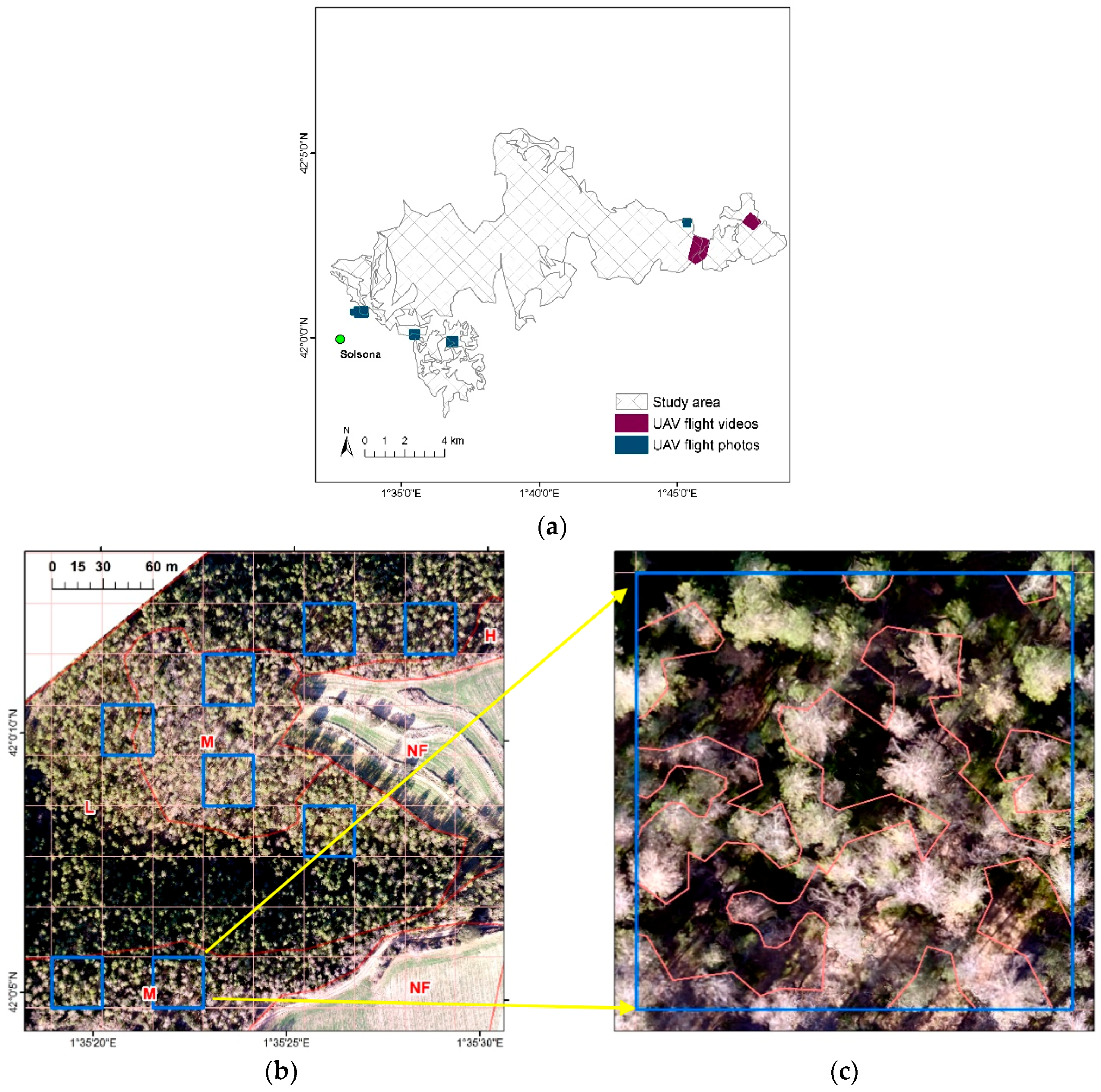
Figure 2.
Observed defoliations based on UAV imagery showing: (a) the location of UAV sample images captured in photos and videos where sketch map polygons were identified as most severely affected areas in 2016; (b) an example of the orthomosaic stratified by land cover and defoliation degree (NF—not forested, L—low, M—medium, H—high) showing selected grid cells of 30 m × 30 m; (c) visual interpretation of defoliation in percentage per grid cell (50% in this sample).

Figure 3.
Scatterplots of defoliation (%) as response variable and dVI as predictor variable: (a) dMID; (b) dMSI; (c) dNDMI; (d) dNDVI; (e) dNBR.
Figure 3.
Scatterplots of defoliation (%) as response variable and dVI as predictor variable: (a) dMID; (b) dMSI; (c) dNDMI; (d) dNDVI; (e) dNBR.

Figure 4.
Severity map of defoliation classified by threshold limits of dMSI representing pine-dominant stands (excluding non-forested areas and stands dominated by other tree species).
Figure 4.
Severity map of defoliation classified by threshold limits of dMSI representing pine-dominant stands (excluding non-forested areas and stands dominated by other tree species).


Table 1.
Vegetation indices derived from Landsat 8 multispectral bands.
| Index | Acronym | Formula | Reference |
|---|---|---|---|
| Middle Infrared Wavelengths | MID | Band 6 + Band 7 | [28] |
| Moisture Stress Index | MSI | [29] | |
| Normalized Difference Moisture Index | NDMI | [30] | |
| Normalized Difference Vegetation Index | NDVI | [31] | |
| Normalized Burn Ratio | NBR | [32] |
Table 2.
Selected UAV sample images for calibration in each category of defoliation severity.
| Severity | Defoliation (%) | Number of Samples |
|---|---|---|
| Nil | 0–5 | 10 |
| Low | 10–30 | 23 |
| Medium | 35–65 | 8 |
| High | 70–100 | 9 |
Table 3.
Summary of logistic regression models.
| Index | Equation | R2 (McFadden’s) |
|---|---|---|
| dMID | 0.740 | |
| dMSI | 0.815 | |
| dNDMI | 0.749 | |
| dNDVI | 0.787 | |
| dNBR | 0.776 |
Table 4.
Threshold limits and the range of vegetation indices.
| Index | Defoliation (%) | ||
|---|---|---|---|
| 10 | 35 | 70 | |
| dMID | −222 | −599 | −949 |
| dMSI | −125 | −295 | −453 |
| dNDMI | 963 | 2081 | 3121 |
| dNDVI | 743 | 1636 | 2466 |
| dNBR | 1034 | 2172 | 3229 |
Table 5.
Confusion matrix of a threshold classification using 50 pixel values of dMSI predicted from Landsat 8 in reference to four classes observed from UAV.
Table 5.
Confusion matrix of a threshold classification using 50 pixel values of dMSI predicted from Landsat 8 in reference to four classes observed from UAV.
| Class | Predicted (Landsat 8) | ||||||
|---|---|---|---|---|---|---|---|
| Nil | Low | Medium | High | Total | Producer’s Accuracy | ||
| Observed (UAV) | Nil | 9 | 1 | 0 | 0 | 10 | 0.90 |
| Low | 2 | 17 | 4 | 0 | 23 | 0.74 | |
| Medium | 0 | 3 | 4 | 1 | 8 | 0.50 | |
| High | 0 | 0 | 3 | 6 | 9 | 0.67 | |
| Total | 11 | 21 | 11 | 7 | 50 | ||
| User’s Accuracy | 0.82 | 0.81 | 0.36 | 0.86 | 0.72 | ||
© 2018 by the authors. Licensee MDPI, Basel, Switzerland. This article is an open access article distributed under the terms and conditions of the Creative Commons Attribution (CC BY) license (http://creativecommons.org/licenses/by/4.0/).
Share and Cite
MDPI and ACS Style
Otsu, K.; Pla, M.; Vayreda, J.; Brotons, L. Calibrating the Severity of Forest Defoliation by Pine Processionary Moth with Landsat and UAV Imagery. Sensors 2018, 18, 3278. https://doi.org/10.3390/s18103278
AMA Style
Otsu K, Pla M, Vayreda J, Brotons L. Calibrating the Severity of Forest Defoliation by Pine Processionary Moth with Landsat and UAV Imagery. Sensors. 2018; 18(10):3278. https://doi.org/10.3390/s18103278
Chicago/Turabian StyleOtsu, Kaori, Magda Pla, Jordi Vayreda, and Lluís Brotons. 2018. "Calibrating the Severity of Forest Defoliation by Pine Processionary Moth with Landsat and UAV Imagery" Sensors 18, no. 10: 3278. https://doi.org/10.3390/s18103278
Note that from the first issue of 2016, this journal uses article numbers instead of page numbers. See further details here.