Multi-Sensor Based Online Attitude Estimation and Stability Measurement of Articulated Heavy Vehicles


Abstract
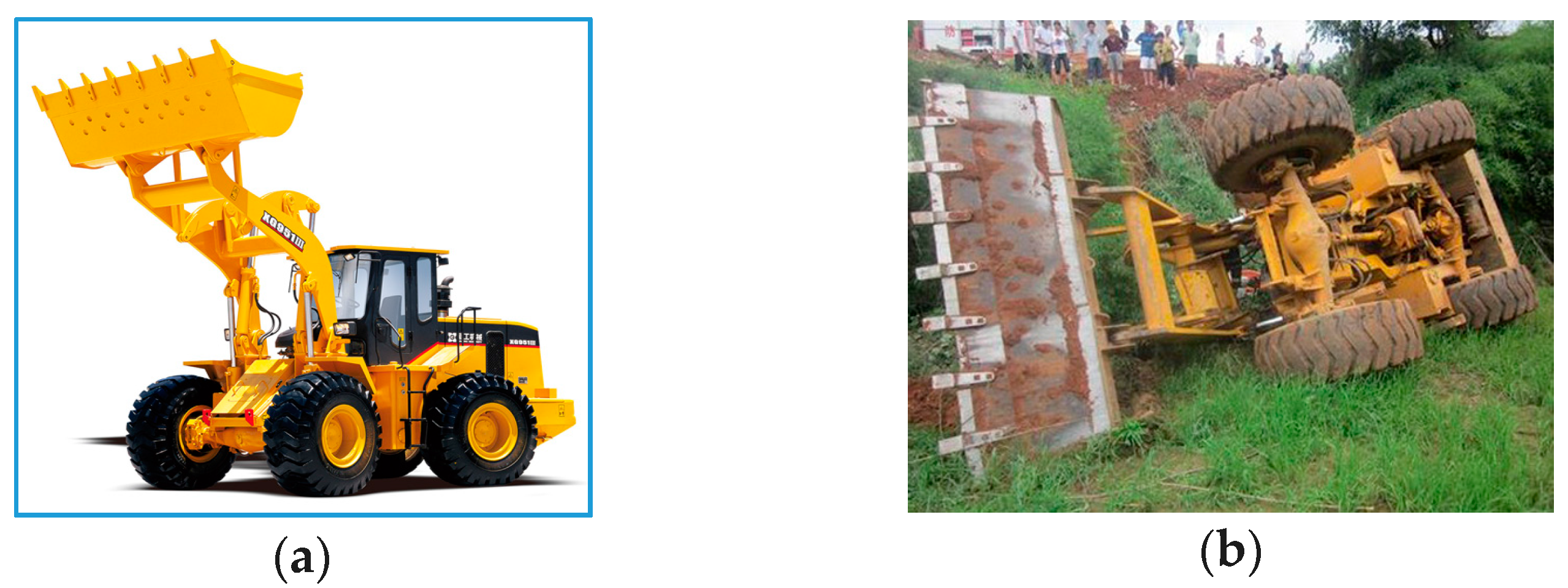
:1. Introduction
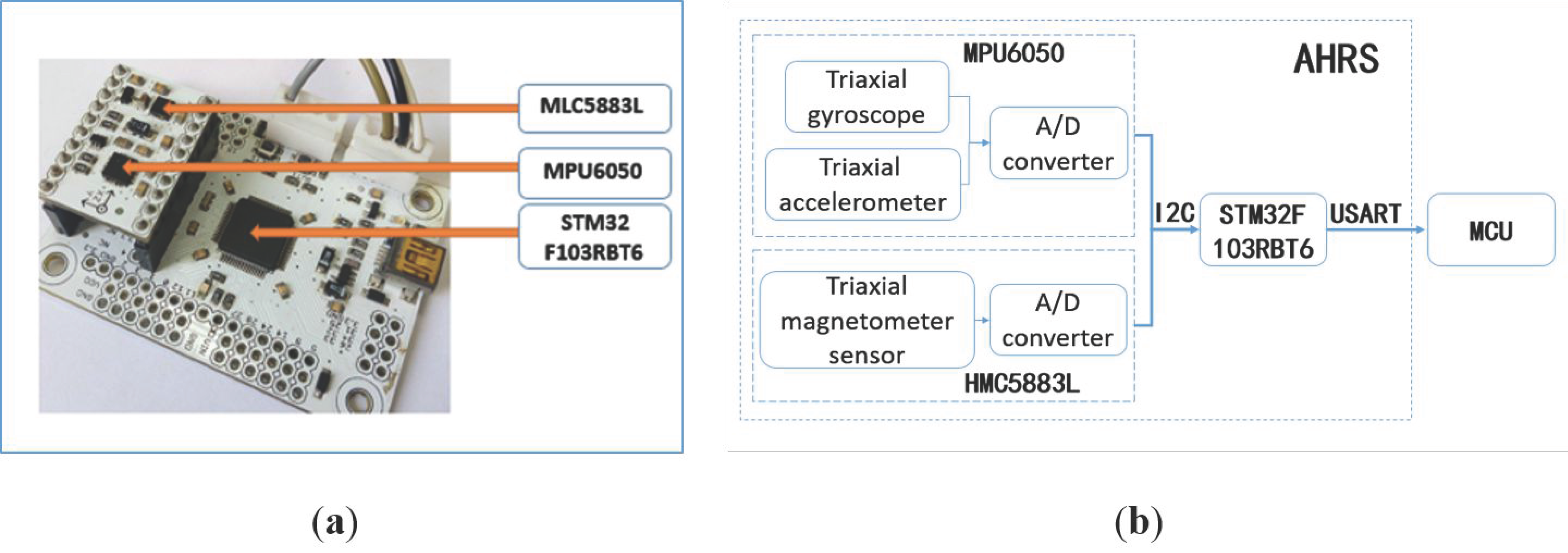
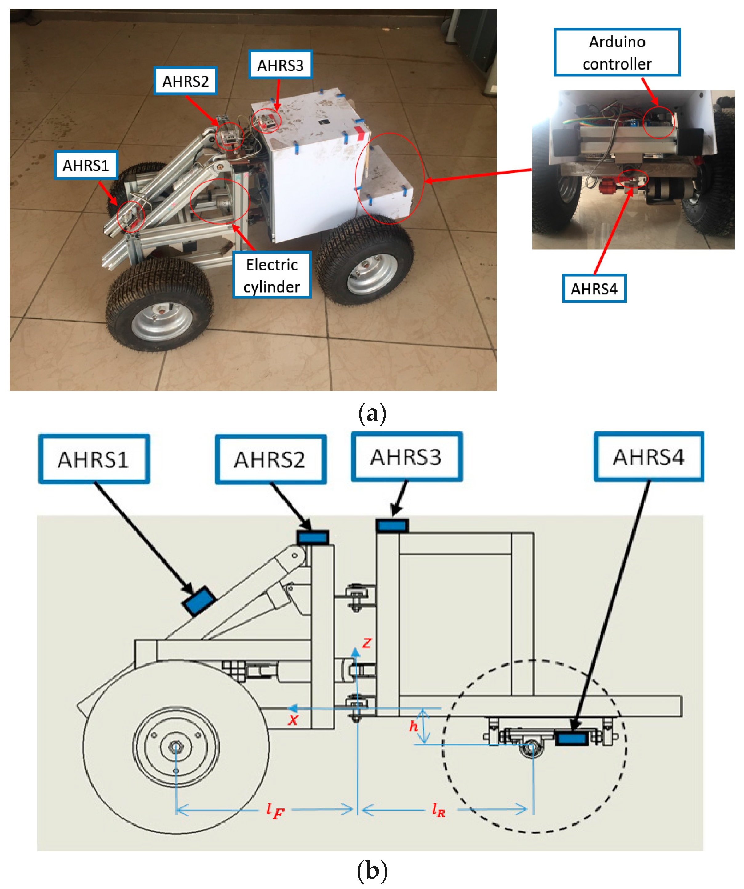
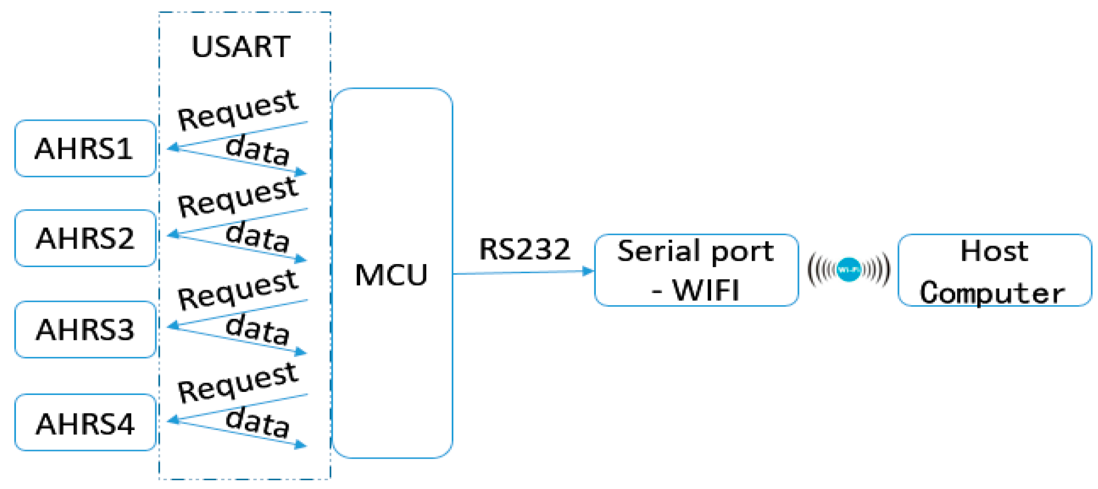
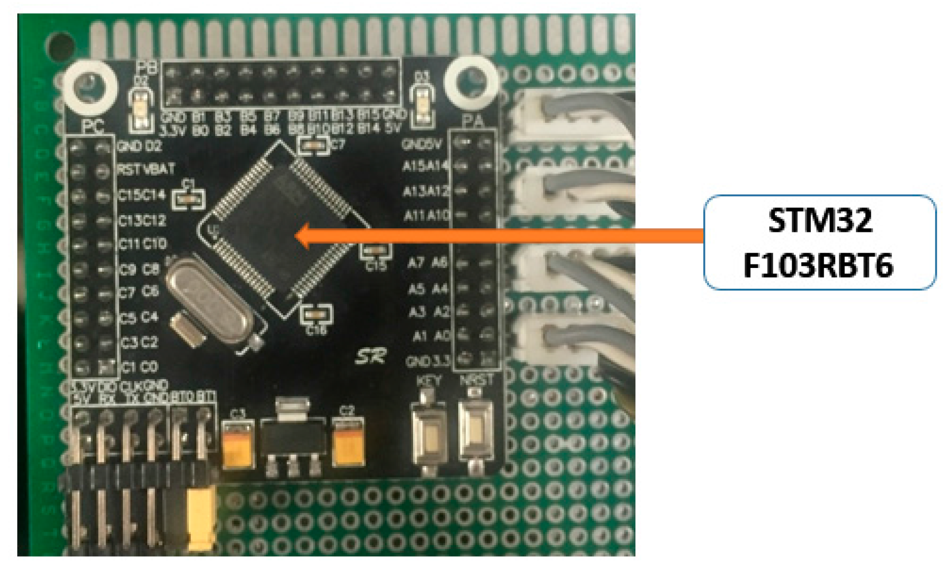
2. Measurement System Construction
3. SSMA Measurement Based on AHRS
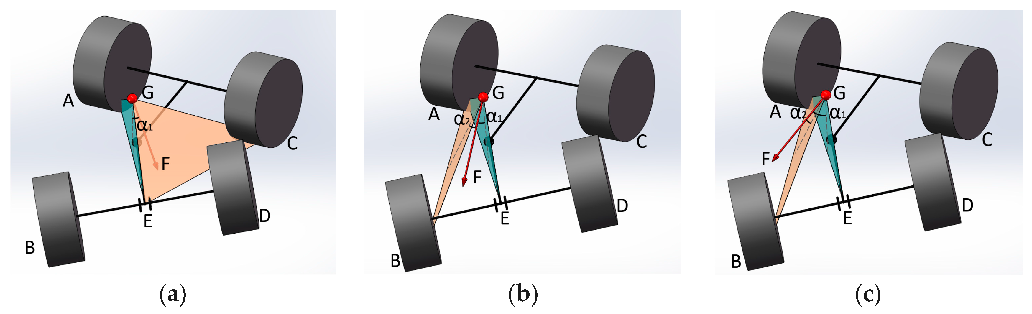
3.1. SSMA Definition
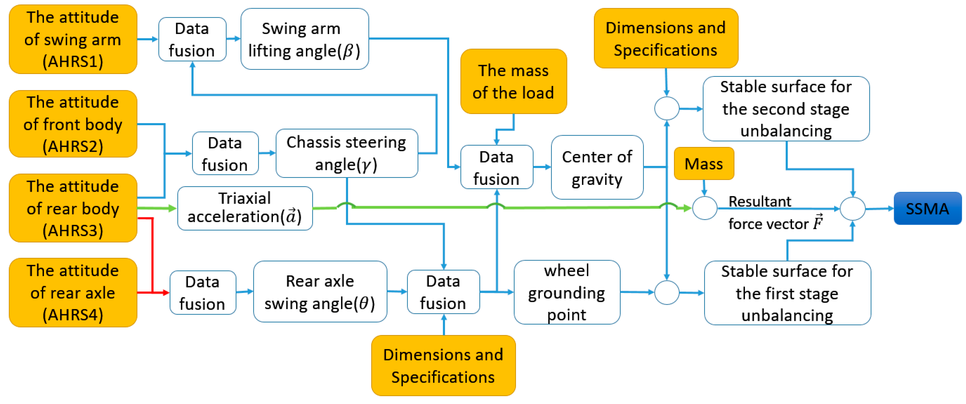
3.2. Measurement Principle
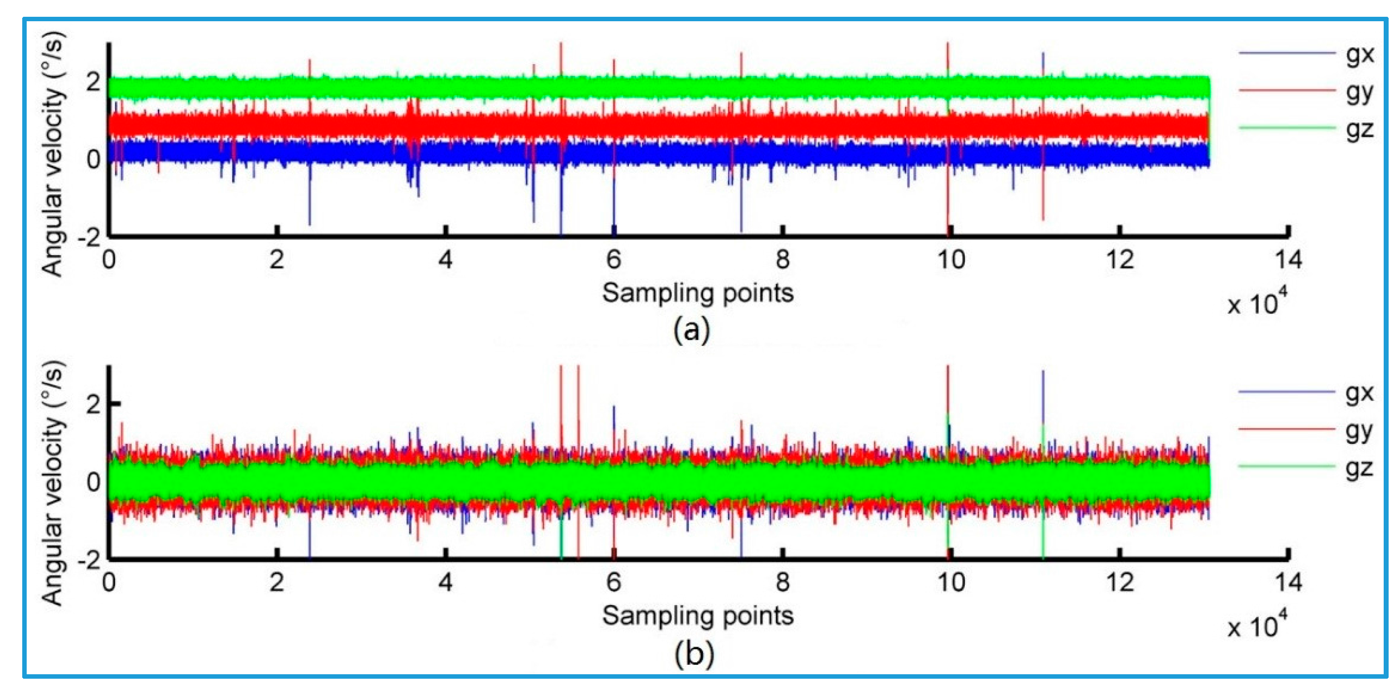
3.3. Measurement Accuracy Calibration of AHRS
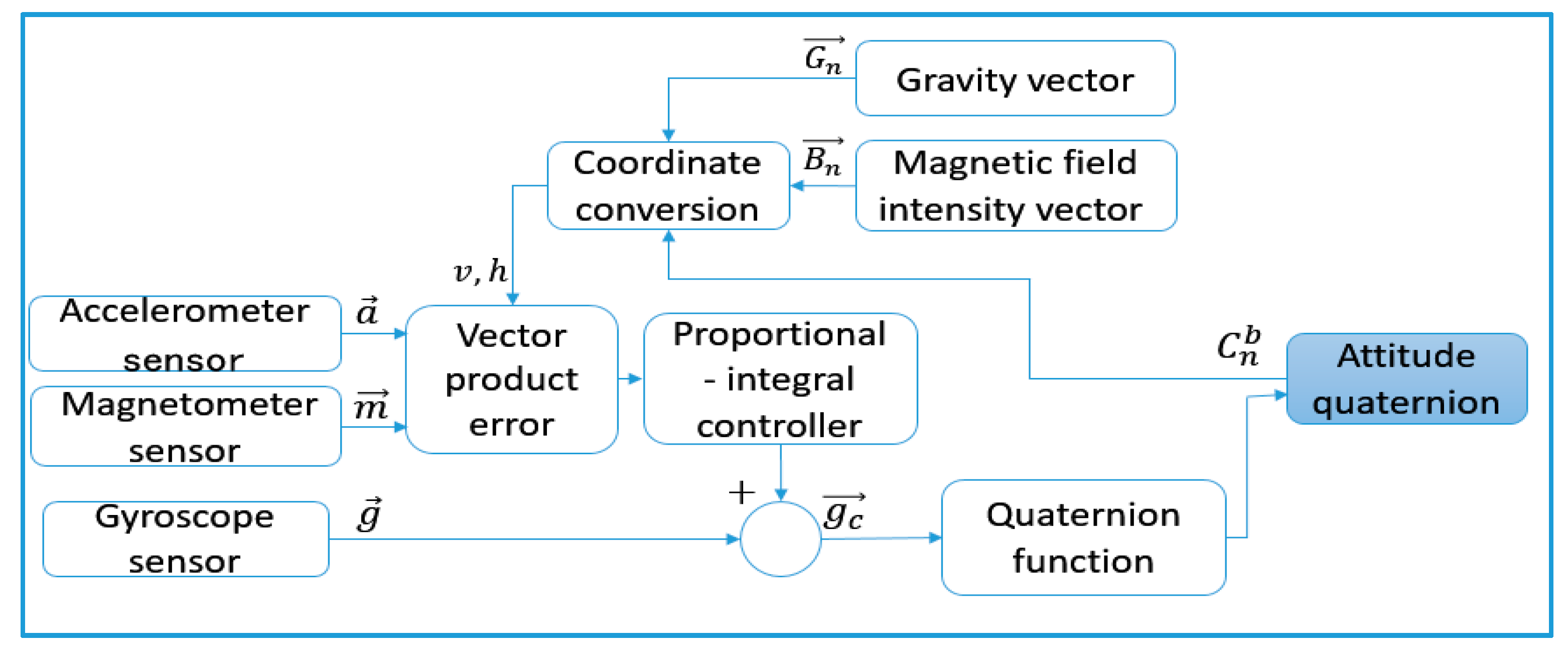
3.3.1. Complementary Filtering Algorithm
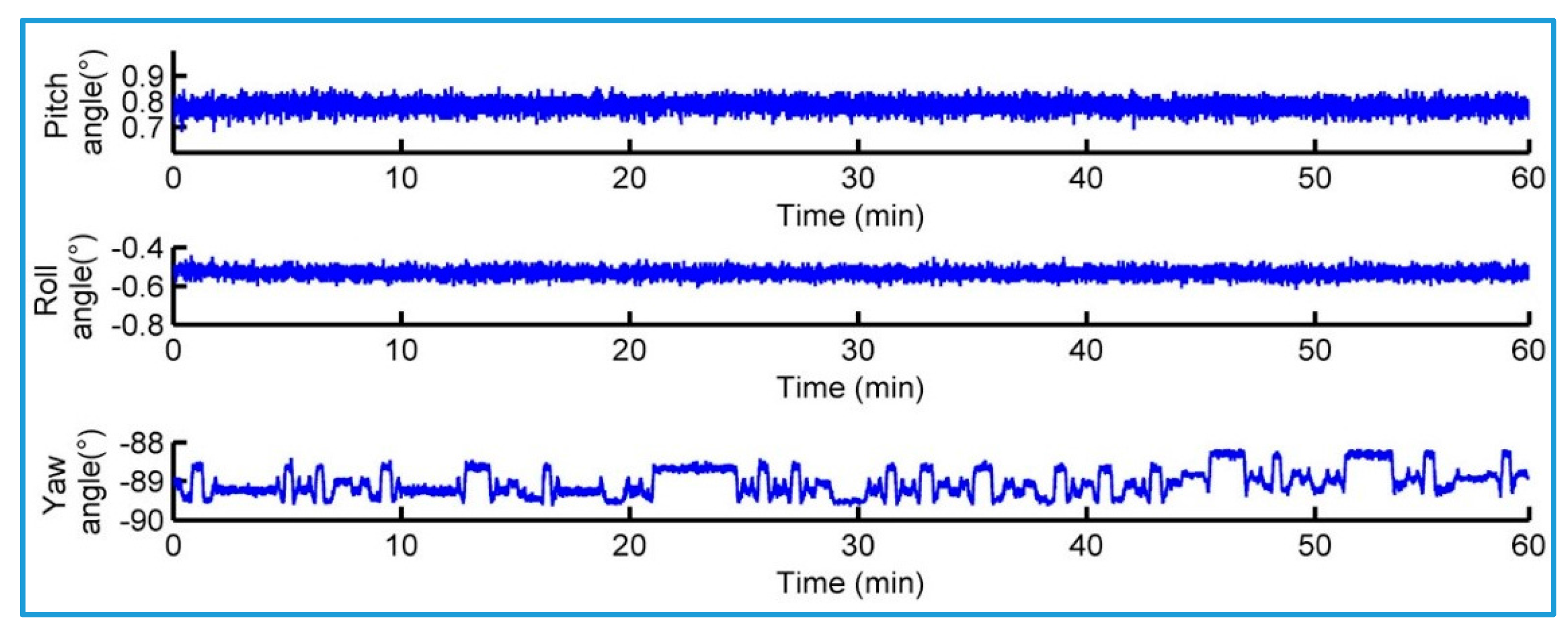
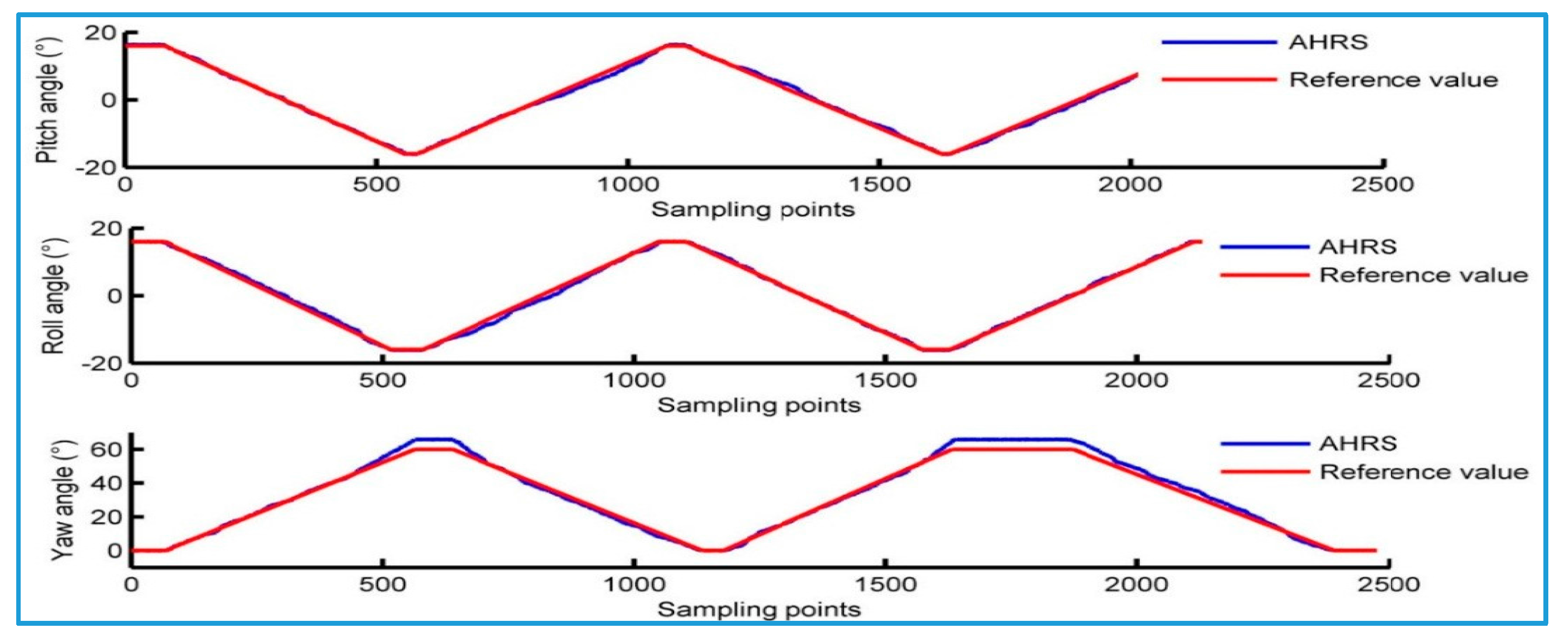
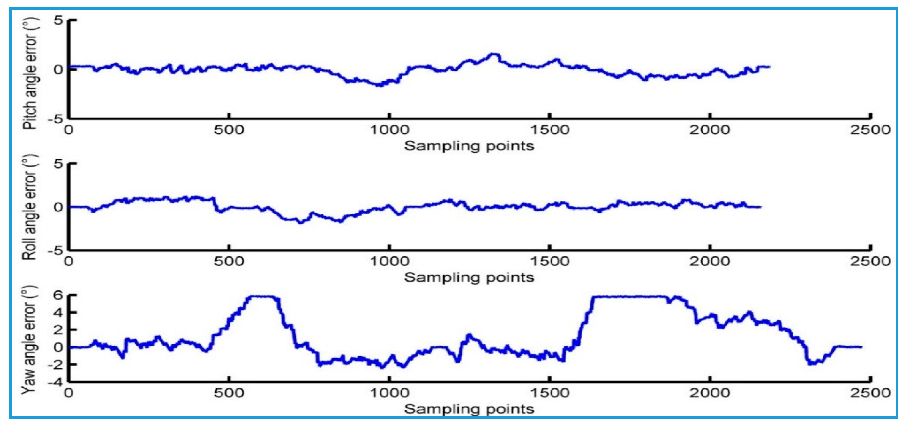
3.3.2. AHRS Calibration Results
4. Lateral Tilting Test and Data Analysis Results
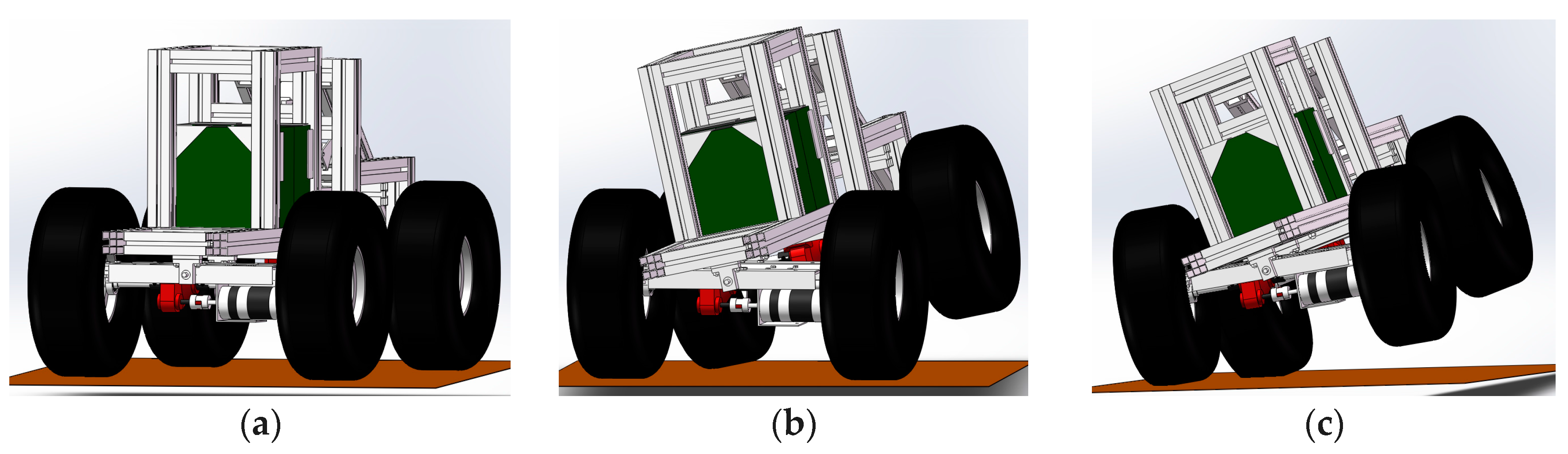
4.1. Static Test
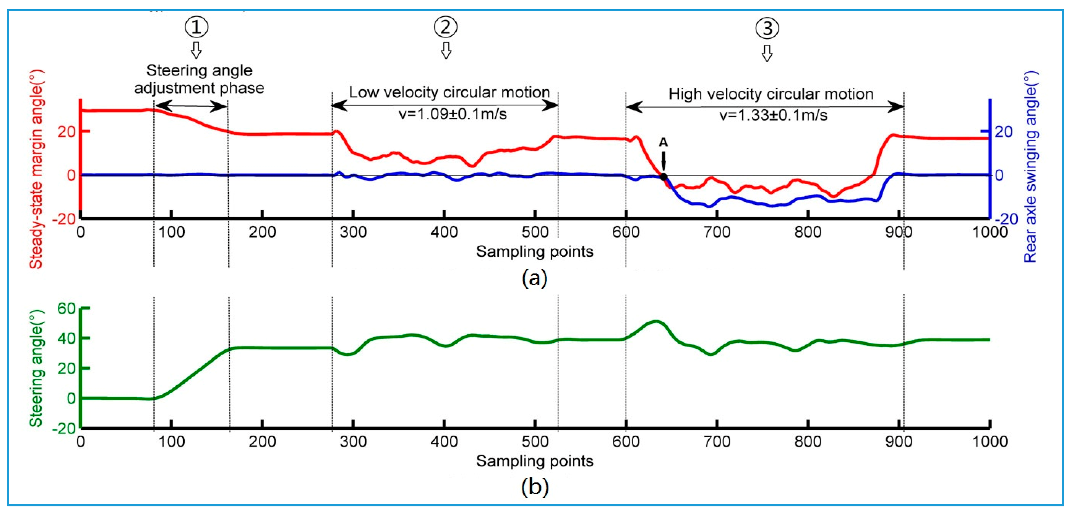
4.2. Dynamic Test
5. Conclusions
Acknowledgments
Author Contributions
Conflicts of Interest
Appendix A
| Algorithm: The Algorithm for SSMA Calculation |
| //The data acquisition algorithm is used to extract all sensor data; Generate Date List, Status list; Get all the date points , and put them in the Date List; Get all the status values , and put them in the Status list; ; ; For j = 0 to Date List.num do Start the timer; Send to; If , wait until the time end and get back; end If; Update the ; End //The calculation for SSMA Generate Date List, Status list; Get all the date points , and put them in the Date List; Get the status value in , and put it in the Status list; Put the default status value in the Status list; If , decode the , and save it to the queue, save the initial data ; If , get to calculate the angel of movable arm, and save it to Date List; If , get to calculate the steering angel, and save it to Date List; If , get to calculate the swing angel, and save it to Date List; Get all them out including to calculate SSMA, and save it to Date List; End If Update the, Update SSMA; End. |
Appendix B
| Algorithm: The Algorithm for Complementary Filtering |
| //Complementary algorithm; Generate Date List, Status list; Get all the date points , and put them in the Date List; Get all the status values , and put them in the Status list; For j = 0 to Date List.num do Get the out to calculate ; If ; ; Calculate; End If. |
References
- Rehnberg, A. Vehicle Dynamic AAnalysis of Wheel Loaders with Suspended Axles. Ph.D. Thesis, Royal Institute of Technology, Stockholm, Sweden, 2008. [Google Scholar]
- Available online: http://www.qihuiwang.com/product/q33310/157848.html (accessed on 10 January 2018).
- Available online: http://119.china.com.cn/qxjy/txt/2012-06/27/content_5115836.htm (accessed on 10 January 2018).
- Palkovics, L.; Semsey, A.; Gerum, E. Roll-over prevention system for commercial vehicles–additional sensorless function of the electronic brake system. Veh. Syst. Dyn. 1999, 32, 285–297. [Google Scholar] [CrossRef]
- Chen, B.-C.; Peng, H. Differential-braking-based rollover prevention for sport utility vehicles with human-in-the-loop evaluations. Veh. Syst. Dyn. 2001, 36, 359–389. [Google Scholar] [CrossRef]
- Mcghee, R.B.; Iswandhi, G.I. Adaptive locomotion of a multi-legged robot over rough terrain. IEEE Trans. Syst. Man Cybern. 1979, 9, 176–182. [Google Scholar] [CrossRef]
- Papadopoulos, E.; Rey, D.A. The force-angle measure of tipover stability margin for mobile manipulators. Veh. Syst. Dyn. 2000, 33, 29–48. [Google Scholar] [CrossRef]
- Nalecz, A.G.; Bindemann, A.C.; Bare, C. Sensitivity analysis of vehicle tripped rollover model. No. NAL-UMC-788. 1988. [Google Scholar]
- Nalecz, A.G. Influence of vehicle and roadway factors on the dynamics of tripped rollover. Tech. Phys. Lett. 1989, 24, 94–96. [Google Scholar]
- Moshchuk, N.K.; Chen, S.K.; Chen, C.F. Roll Stability Indicator for Vehicle Rollover Control. U.S. Patent 7,788,007, 31 August 2010. [Google Scholar]
- Iagnemma, K.; Rzepniewski, A.; Dubowsky, S.; Schenker, P. Control of robotic vehicles with actively articulated suspensions in rough terrain. Autonom. Robot. 2003, 14, 5–16. [Google Scholar] [CrossRef]
- Peter, S.C.; Iagnemma, K. Stability measurement of high-speed vehicles. Veh. Syst. Dyn. 2009, 47, 701–720. [Google Scholar] [CrossRef]
- Rakheja, S.; Piché, A. Development of directional stability criteria for an early warning safety device. Sea Pap. 1990. [Google Scholar] [CrossRef]
- Kamnik, R.; Boettiger, F.; Hunt, K. Roll dynamics and lateral load transfer estimation in articulated heavy freight vehicles. Proc. Inst. Mech. Eng. Part D J. Automob. Eng. 2003, 217, 985–997. [Google Scholar] [CrossRef]
- Miege, A.J.P.; Cebon, D. Active roll control of an experimental articulated vehicle. Proc. Inst. Mech. Eng. Part D J. Automob. Eng. 2005, 219, 791–806. [Google Scholar] [CrossRef]
- Jin, Z.L.; Weng, J.S.; Hu, H.Y. Rollover stability of a vehicle during critical driving manoeuvres. Proc. Inst. Mech. Eng. Part D J. Automob. Eng. 2007, 221, 1041–1049. [Google Scholar] [CrossRef]
- Larish, C.; Piyabongkarn, D.; Tsourapas, V.; Rajamani, R. A new predictive lateral load transfer ratio for rollover prevention systems. IEEE Trans. Veh. Technol. 2013, 62, 2928–2936. [Google Scholar] [CrossRef]
- Jin, Z.; Zhang, L.; Zhang, J.; Khajepour, A. Stability and optimized H∞ control of tripped and untripped vehicle rollover. Veh. Syst. Dyn. 2016, 54, 1–23. [Google Scholar] [CrossRef]
- Li, X.; Wu, Y.; Zhou, W.; Yao, Z. Study on roll instability mechanism and stability index of articulated steering vehicles. Math. Probl. Engeerg 2016, 2016, 1–15. [Google Scholar] [CrossRef]
- Zhu, Q.; Yi, J.; Chen, H.; Wen, C.; Hu, H. Lateral stability simulation and analysis for wheel loaders based on the steady-state margin angle. Int. J. Model. Identif. Control 2014, 22, 185–194. [Google Scholar] [CrossRef]
- Nygren, E.; Sitaraman, R.K.; Sun, J. The Akamai network: A platform for high-performance internet applications. ACM Sago’s Oper. Syst. Rev. 2010, 44, 2–19. [Google Scholar] [CrossRef]
- De Vito, S.; Palma, P.D.; Ambrosino, C.; Massera, E. Wireless sensor networks for distributed chemical sensing: Addressing power consumption limits with on-board intelligence. IEEE Sens. J. 2011, 11, 947–955. [Google Scholar] [CrossRef]
- Lai, Y.C.; Jan, S.S.; Hsiao, F.B. Development of a low-cost attitude and heading reference system using a three-axis rotating platform. Sensors 2010, 10, 2472–2491. [Google Scholar] [CrossRef] [PubMed]
- Madgwick, S.O.H.; Harrison, A.J.L.; Vaidyanathan, R. Estimation of Imu and Marg Orientation Using a Gradient Descent Algorithm. In Proceedings of the 2011 IEEE International Conference on Rehabilitation Robotics, Zurich, Switzerland, 29 June–1 July 2011. [Google Scholar]
- Fourati, H. Heterogeneous data fusion algorithm for pedestrian navigation via foot-mounted inertial measurement unit and complementary filter. IEEE Trans. Instrum. Meas. 2015, 64, 221–229. [Google Scholar] [CrossRef]
- Carminati, M.; Ferrari, G.; Grassetti, R.; Sampietro, M. Real-time data fusion and MEMS sensors fault detection in an aircraft emergency attitude unit based on Kalman filtering. IEEE Sens. J. 2011, 12, 2984–2992. [Google Scholar] [CrossRef]
- Li, X.; Li, Z. Vector-aided in-field calibration method for low-end mems gyros in attitude and heading reference systems. IEEE Trans. Instrum. Meas. 2014, 63, 2675–2681. [Google Scholar] [CrossRef]
- Sipos, M.; Paces, P.; Rohac, J.; Novacek, P. Analyses of tri-axial accelerometer calibration algorithms. IEEE Sens. J. 2012, 12, 1157–1165. [Google Scholar] [CrossRef]
- DIN ISO. Road Vehicles—Steady State Circular Test Procedure; DIN ISO 4138-1984; DIN ISO: Berlin, Germany, 1984. [Google Scholar]


| Principle of Indicators | Advantages | Disadvantages |
|---|---|---|
| Geometric principle | Simple principle | Ignore the changes in the height of the vehicle center of weight and the dynamic performance of the vehicle on its stability |
| Rollover energy | For tripping rollover | Ignore the various aspects of energy consumption in the rollover process |
| Contact force between tire and ground | Intuitively represent the stability of the vehicle | Tire ground contact force is difficult to accurately measure |
| Static threshold | Convenient and direct accurate | The warning performance is poor |
| Combination indicators | More reasonable and comprehensive represent of the vehicle rollover stability | Too many parameters need to be detected |
| Parameter | Explanation | Value |
|---|---|---|
| total mass of the prototype | 56.1 | |
| front body mass | 16.4 | |
| rear body mass | 26.4 | |
| rear axle mass | 13.3 | |
| moment of inertia of front body | 0.642,1.57,1.68 | |
| moment of inertia of rear body | 0.765,1.79,1.25 | |
| moment of inertia of rear axle | 0.413,1.58,1.89 | |
| center of weight of front body | 0.26,0,0.005 | |
| center of weight of rear body | −0.19,0,0.14 | |
| center of weight of rear axle | −0.33,0,−0.04 | |
| wheel track | 0.45 | |
| distance between pivot joint and the center of the front axle | 0.32 | |
| distance between pivot joint and the center of the rear axle | 0.32 | |
| tire radius | 0.15 | |
| distance between rear axle shaft and rear body longitude axis | 0.02 | |
| cornering stiffness of tire | 81,600 | |
| vertical stiffness of tire | 20,000 | |
| vertical damping of tire | 5000 |
| Parameter | Define |
|---|---|
| center of weight point | |
| the resultant force of weight and inertia force of the loader that acts on center of weight point G | |
| A | left front wheel grounding point |
| B | left rear wheel grounding point |
| C | right front wheel grounding point |
| D | right rear wheel grounding point |
| E | the panel point of rear body and rear axle |
| the angle between and the plane △GAE (or △GCE) | |
| the angle between and the plane △GAB (or △GCD) |
© 2018 by the authors. Licensee MDPI, Basel, Switzerland. This article is an open access article distributed under the terms and conditions of the Creative Commons Attribution (CC BY) license (http://creativecommons.org/licenses/by/4.0/).
Share and Cite
Zhu, Q.; Xiao, C.; Hu, H.; Liu, Y.; Wu, J. Multi-Sensor Based Online Attitude Estimation and Stability Measurement of Articulated Heavy Vehicles. Sensors 2018, 18, 212. https://doi.org/10.3390/s18010212
Zhu Q, Xiao C, Hu H, Liu Y, Wu J. Multi-Sensor Based Online Attitude Estimation and Stability Measurement of Articulated Heavy Vehicles. Sensors. 2018; 18(1):212. https://doi.org/10.3390/s18010212
Chicago/Turabian StyleZhu, Qingyuan, Chunsheng Xiao, Huosheng Hu, Yuanhui Liu, and Jinjin Wu. 2018. "Multi-Sensor Based Online Attitude Estimation and Stability Measurement of Articulated Heavy Vehicles" Sensors 18, no. 1: 212. https://doi.org/10.3390/s18010212
APA StyleZhu, Q., Xiao, C., Hu, H., Liu, Y., & Wu, J. (2018). Multi-Sensor Based Online Attitude Estimation and Stability Measurement of Articulated Heavy Vehicles. Sensors, 18(1), 212. https://doi.org/10.3390/s18010212