The construction and maintaining of the spanning tree, which is the core of our approach, is based on dynamic leader election, commonly studied in the field of fault tolerant distributed agreement [
12,
22,
23]. We present two alternative protocols to implement this approach. The first one (
Subsection 3.2.1) uses a reactive, asynchronous forwarding mechanism to propagate leader election messages. Differently, the second protocol (
Subsection 3.2.2) piggybacks the messages on periodic heartbeats messages.
3.1. Notation and Assumptions
We consider an architecture with an unknown set of n resource-constrained mobile sensor nodes and one more powerful mobile sink. We denote this set of sensor nodes as . When required for simplicity, we will also refer to a node as p, q, etc. We will denote as s the sink node. Every node of the system has a unique identifier and a local clock to measure real-time intervals.
Every node, including the sink node, can move. The mobility of a node is characterized according to two dimensions: velocity and direction. At any time t, a node p moves towards some direction with a velocity , being the maximum velocity of every node p in the system.
A node can leave the system, due to a fault or disconnection, or join the system. Connections and disconnections can be caused by mobility, as the node enters and comes out of the communication range of other nodes in the system, or for other reasons. In the following, we formalise this concept.
Every node uses broadcast communication to exploit the Wireless Broadcast Advantage (WBA) [
18]. At any time
t, a node
p can communicate directly (i.e., at one hop) with a subset
, which are the nodes that are at time
t into a radius
r from
p, also referred as the neighbourhood of
p. The communication range
r is a common parameter for all nodes in
V. For simplicity, we consider that message transmission delays are bounded.
We define the parameter link quality as a measure of the transmission power (in ), which can be easily extracted in a node p at the reception of a message by p from q. We will use the notation to refer to the link quality for a link at time t. We assume that . We define as the threshold for the RSSI (Received Signal Strength Indicator) such that a link can be considered to have good link quality.
When considering link quality, a graph representing the connectivity conditions in V at time t is obtained. We also define a spanning tree . Ideally, will include only links with good link quality.
Observe that partitions in are possible, but we assume that , . A node p can be disconnected from due to either: (a) , or (b) .
3.2. Building the Communication Tree
The goal of our approach is to provide an efficient communication route from any node p to the root node s in scenarios where sensor devices are mobile. To do so, our approach creates a spanning tree with the root in the sink node s. The spanning tree is continuously maintained in order to represent the best routing options at time t on the basis of the link quality information, providing a foundation for efficient routing by maximising the probabilities of successful communications, and henceforth increasing message delivery rates and reducing communication costs.
Figure 1a–f illustrate how a spanning tree is built in situations of node movement, the arrival of a new node (
Figure 1d), or a disconnection (
Figure 1f).
We now describe the algorithmic details of the approach. First, we focus on the common features of the two alternative protocols we propose in this work. Then, we devote two specific subsections to describe the different mechanisms used in each of the protocols. Please refer, for example, to the first of the protocols (Algorithms 1 and 2) to check the details of the common description.
Both protocols are based on a broadcast primitive. Note that, apart from providing energy-efficiency in the multi-hop information dissemination [
18], broadcast is also useful to detect changes in the neighbourhood.
The sink node s is in charge of generating new rounds in the spanning tree reconfiguration. The spanning tree is created from the sink node s, which is the root of the tree, to the rest of nodes. In this regard, s sends leader messages with refreshed round numbers each time (see Algorithm 2). Every node is continuously listening to the communication channel.
Every node proposes its leader, denoted . Leader election is executed at every node at time t such that and has the minimum distance to s in the spanning tree . Ties are broken on the basis of the node identifier.
The explicit perception that a node has about its connection with s is another common feature of both protocols. This perception is represented by the variable , which is when is connected. This explicit knowledge of connectivity is provided by the monitorization of the sink node s using the timer . Each time a node receives a new round identifier, re-sets again the timer, denoting as connected. Otherwise, if expires, will consider itself as not connected.
Observe that, while the round identifiers created by s lower-bounds the interval between two consecutive reconfigurations, upper-bounds the interval between two consecutive reconfigurations.
In the following subsections, we describe the two implementations of our leader-based routing (LBR) approach, namely the reactive, eager version (LBR1) and the synchronous, lazy version (LBR2).
3.2.1. Protocol LBR1
Our first implementation relies on delivering the routing information as soon as possible in a reactive way. In this regard, a node computes the election during a whole round. When a message with a higher round number is received by a node , broadcasts a leader message with the result of the previous round computation and the increase of the distance received (The distance is extracted from contextual information stored in the message.) (see Lines 5–11, of Algorithm 1). Thus, sends its own leader message using the last distance to s known by . Observe in Algorithm 2 that no other node but s will send in its leader message a zero distance value.
These new leader messages sent by is essential for multi-hop scenarios. First, leader messages propagate the existence of a sink node in the system. Second, the periodic broadcast of the leader message allows for other nodes to become connected. Finally, leader messages provide the required information to its neighbourhood to create the spanning tree. Consequently, the reception of a new round identifier from s by a node enables a new election round in every , which eventually results in a reconfiguration of the spanning tree.
| Algorithm 1: The algorithm LBR1 executed by any sensing node . Lines 26–38 are also shared with LBR2. |
![Sensors 17 01587 i001]() |
| Algorithm 2: Algorithm executed by the sink node s. |
![Sensors 17 01587 i002]() |
The fact that the sink node broadcasts
leader messages periodically (Algorithm 2) allows for a timer-based monitoring of connectivity changes. The first time that a node
receives a
leader message (let us say, at time
t) from any
,
becomes connected and will remain connected during the time interval
(The
variable has a common value slightly higher than
in order to prevent premature time outs.) by setting the timer
by Line 11. In this way, every
will become connected by Lines 21–24 and will change their variable
pointing to
s (Lines 7 and 8). If
does not receive a new round identifier timely, then, either
will shortly receive a new message by any other path, setting again
by Line 11 and reconfiguring the spanning tree, or, otherwise,
is no longer connected to the spanning tree
. In the last situation, the no reception of a new round identifier will cause
to expire and
will become not connected. Thus, the
variable represents the uncertainty of
to be connected to
s and the expiration of
results in
not connected (Lines 26 and 28).
Figure 1e,f illustrate this situation for node
.
3.2.2. Protocol LBR2
Observe than in our second protocol version, LBR2 (Algorithm 3), the broadcast at Line 6 of LBR1 in
Figure 1 has been removed. Instead, in LBR2, we introduce a task executed in every node
to broadcast every
time the current routing information of
when
considers itself as connected (see Lines 30–34 in Algorithm 3). This allows us to adopt a windowed mechanism at the MAC layer and reduce the probability of collision in communications.
| Algorithm 3: The modifications required by LBR2 to the previous algorithm to be executed by any sensing node . |
![Sensors 17 01587 i003]() |
Additionally, in this second protocol, we modify the leadership criteria as follows. The node will be the one with the lowest distance to s that firstly communicates with . This mechanism is a novel strategy that allows balancing the energy consumption in intermediate nodes at routing time. If many of the nodes share the same , this leader will eventually saturate and the system performance will decrease in terms of battery. To correctly load balance the spanning tree, in LBR2, we introduce an extra timer to monitor the current parent node. This is set when a new node is adopted by (Line 15 in Algorithm 3). Since every node sends its information periodically by Line 32, , it will also send a leader message resetting again the by Line 22. On the other hand, if expires (Lines 27–29), is allowed to re-elect another among those that have the same distance to s, i.e., the condition in Line 16 is satisfied since has been previously set to false by Line 28.
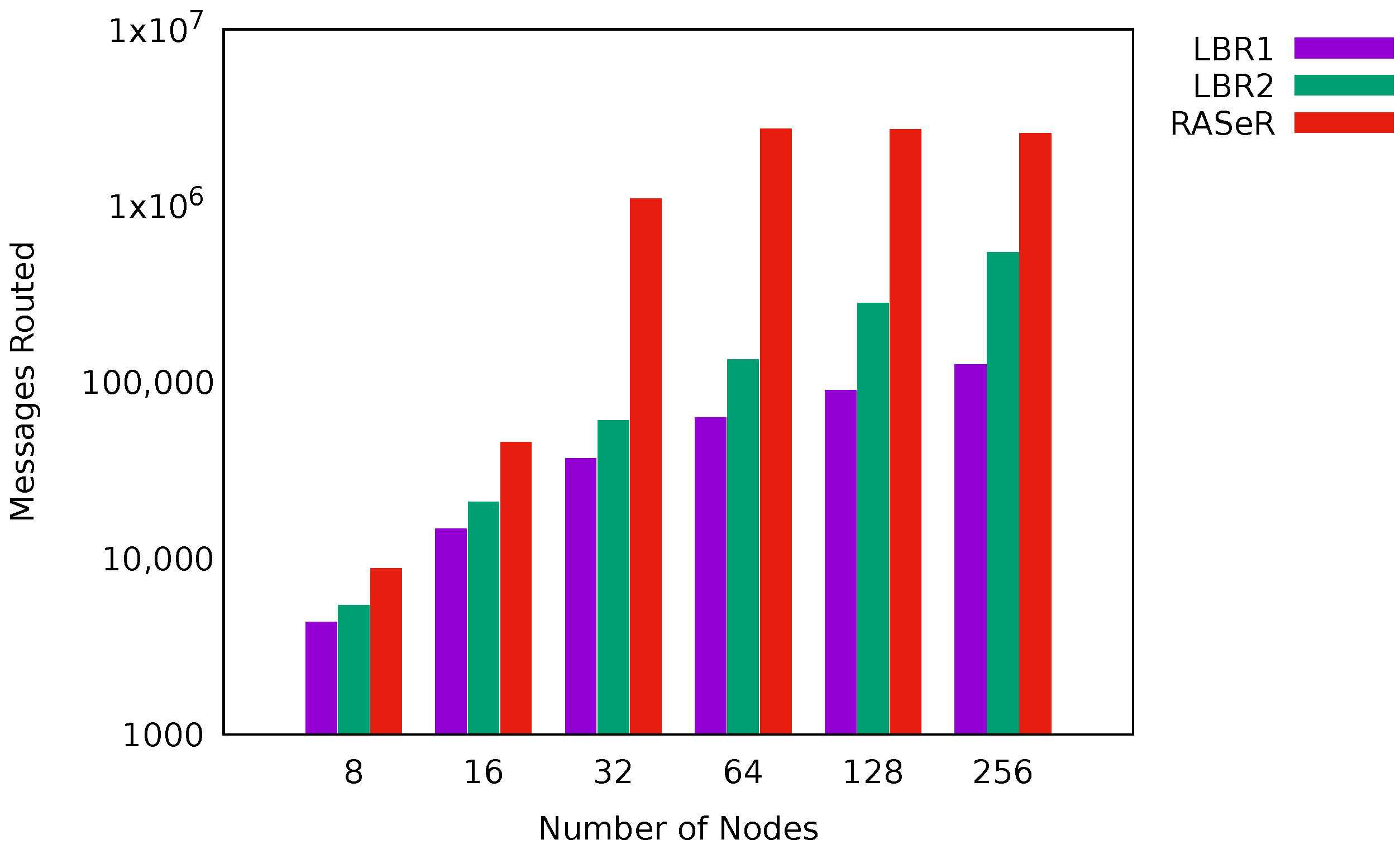
Note that the higher and values are, the slower the graph connectivity change detection is. This introduces a trade-off between the reaction time and the number of messages sent by the system in order to provide good QoS and energy-efficiency at the same time.
Observe also that the global number of messages sent is linear with the number of nodes in the system, which makes LBR2 scalable regarding communication cost.
3.3. Data Routing Protocol
Once an initial spanning-tree has been created, an application-data routing protocol is executed. In contrast to the spanning-tree creation, where we use broadcast as the communication primitive, for application data, we use one-to-one communication.
We have considered two different protocols for sending application data. The first one, which we have adopted in combination with LBR1, consists in the immediate forwarding of the received content to the node (Algorithm 4).
Alternatively, content can be buffered while it is received and be periodically sent piggybacked in leader messages. To do so, the primitive must be redefined as . This approach (Algorithm 5) is the one we have chosen in combination with LBR2.
| Algorithm 4: Direct forwarding strategy executed by node . |
![Sensors 17 01587 i004]() |
| Algorithm 5: Piggybacking strategy executed by node . |
![Sensors 17 01587 i005]() |


