6.1. Simulation Setup
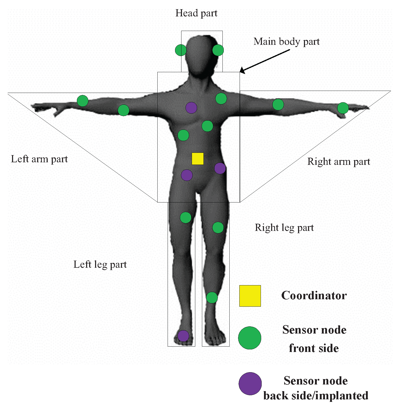
We have conducted simulations based on C++ platform. The WBAN in the simulation consists of one coordinator and 16 sensor nodes. Considering that sensor node executing a certain sensing task may not be always deployed at the same position but in a designated area, in order to show generality of sensor node deployment, we classify the human body into six parts in the simulations as shown in
Figure 1, which contains head part, main body part, left/right arm part and left/right leg part. The range values of each part are measured from a male human body whose height is 175 cm. In the simulations, we deploy six sensor nodes in main body part and two sensor nodes for every other parts. Sensor nodes are randomly deployed in the parts where they belong. Considering the possible implanted sensors or sensor nodes deployed in the backside of human body, we set the ratio of implanted/back side sensors to the total sensor nodes in the network to 25%.
The node distribution is decided based on the functionality each part contains referring to the general application scenarios for WBAN, where we sort that the main body part is responsible for tissue monitoring sensing like electrocardiogram (ECG) and capsule endoscope, positioning sensing, motion detection and drug delivery, arm parts for blood oxygen and glucose sensors, leg parts for lactic acid sensing, pressure sensing and, if possible, artificial support and head part for electroencephalogram (EEG) sensing. In addition, accelerator nodes can be deployed in all six parts. On the other hand, the main body part is physically more stable than other parts, so, in reality, functional sensor nodes that can be put either in the main body part or other parts are preferred to be deployed in the main body part. As a result, in the simulation scenario, we deploy more sensor nodes in the main body part since its physical stability and the fact that it contains more kinds of functional sensor nodes than other parts. The detailed information for node distribution and body parts are listed in
Table 1.
Each sensor node generates a fixed-size packet of
k bits in one superframe. In the simulation, we set
k as 1200 bits, which is a typical frame length in WBAN communication according to IEEE 802.15.6 [
8]. In addition, we adopt 128 kbps as the transmission rate specified in the IEEE 802.15.6. Depending on this, slot length is set to 10 ms. One superframe contains 65 transmission slots and its duration is set to be 700 ms considering the beacon frame transmission slot, which is in the available range described in IEEE 802.15.6 as well.
We adopt the parameter values in the Nordic nRF2401 low power single chip transceiver (Oslo, Skøyen, Norway), which is widely used in sensor node communication as the energy consumption parameters in Equations (1) and (2). The value of
n is set to be 3.38 when the channel between transmitter and receiver is LOS (line-of-sight) and 5.9 when channel is NLOS (non-line-of-sight). The values of
n are adopted from the measurement campaign in [
29] and widely used in the WBAN-related literature [
21,
27,
28,
30,
31]. That is, in
Figure 1, the front side sensors get LOS channels with the coordinator while the back side or implanted sensors get NLOS channels with the coordinator. Mean value
for the energy storage distribution is set to 2 J, and we set a 50% offset from the mean value as the upper and lower bound (
J) for the distribution.
When the first sensor node in the WBAN runs out, the simulation stops. The simulation runs for 1000 times, and the averaged results are taken. The system parameters used in the simulation are summarized in
Table 2.
6.2. Result Analysis
Firstly, before the lifetime performance comparison, the time complexity performance of the heuristic solution and its convergency loop condition are analyzed. From a theoretical perspective, when we use the enumeration method to solve the optimization, the time complexity is
. However, when it comes to the proposed heuristic iterative solution, the time complexity is only
. On the other hand, from the experimental perspective in
Table 3, which illustrates the average time cost to solve the optimization in the simulation with the varying number of nodes in the network, the enumeration costs much more than the proposed rapid solution. In more detail, the time taken by enumeration grows very fast with the increasing number of nodes, even more than an hour when the number of nodes is 20 in our simulation. While the proposed solution grows much more smoothly within a hundred microseconds. In a word, the simulation results in
Table 3 match the theoretical analysis on time complexity of enumeration and the proposed solution.
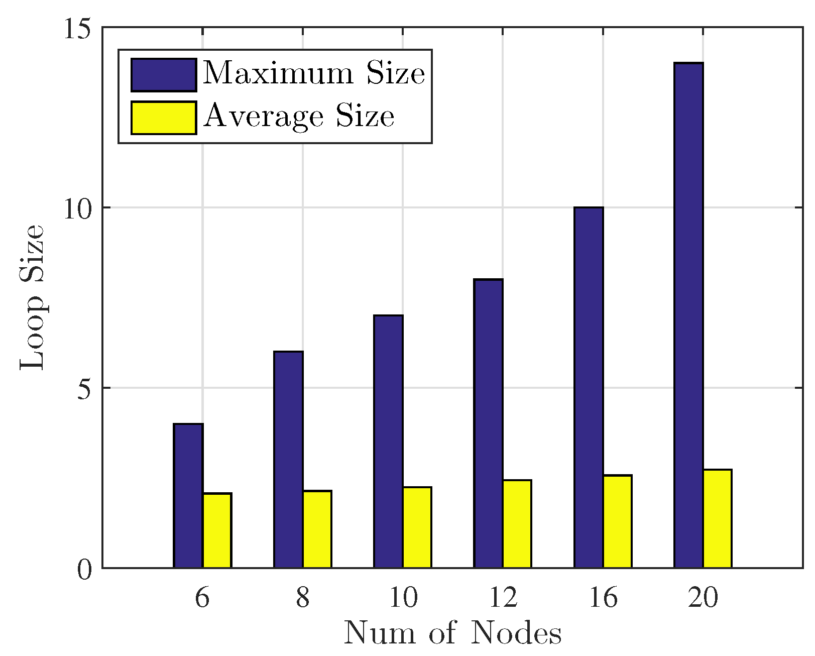
Figure 2 shows the convergency loop performance of the proposed rapid solution when the iteration ended in the simulation. It can be seen from the figure that the proposed solution always converges to a loop no matter how many nodes are involved (if the iteration can not converge to a loop, then the loop size will be represented by
∞), which means that the iteration of the proposed solution can always converge to an end in the simulation. The average loop size is close to 2 which indicates that the majority of the loop size in the simulation is 2. Furthermore, it can be seen that when the number of nodes grows, the maximum and average loop size increase due to the fact that the dimensions of
X become larger, which brings more binary value combinations for the relay selection matrix.
Next, we focus our attention on the performance comparison of network lifetime between our proposed scheme with some existing relay selection schemes: benchmark strategy, where each node in the network only uses direct transmission, the algorithm in [
13] (sum-rate algorithm), which is a popular relay selection scheme in WSNs aiming to minimize the total energy consumption, and the WBAN-specific relay selection algorithm in [
24] (maxi-rate algorithm), which formulates an optimization problem to minimize the maximum energy consumption rate among sensor nodes. In addition, the optimal value obtained from the optimization using enumeration is also presented in the comparison in order to show the performance gap between the proposed solution and the optimal value.
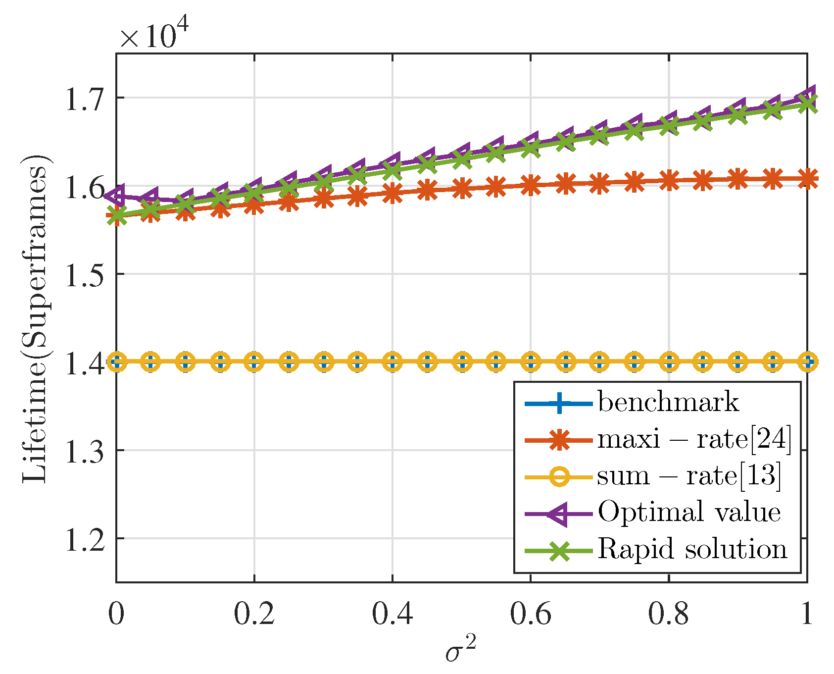
Figure 3 shows the lifetime performance of each algorithm with the variation of
. The larger the value of
is, the more serious the energy inequality in the network that exists. The lifetime on the
y-axis in the unit of superframes represents how many superframes the network gets through before the first sensor node runs out of energy under different relay selection algorithms. That is to say, more superframes means longer lifetime of the network. It can be firstly seen from the figure that the performance of the rapid solution is very close to the optimal value of the optimization. Precisely, the performance gap between the proposed heuristic solution and the optimal value of the optimization is only about 0.5% on average. Combining with the time complexity analysis in
Table 3 and
Figure 2, it can be inferred that the proposed heuristic iteration described in Algorithm 1 is an effective and time-efficient solution to the optimization problem. In addition, it is confirmed that, throughout the simulations in this paper, performance gap between the rapid solution and the optimal value of the optimization is always very small similar with the results shown in
Figure 2. Hence, for simple and clear illustration in the following performance analysis, we will use the results obtained from the rapid solution to represent the performance of LMRSS.
It can be obviously seen from
Figure 3 that LMRSS is always the better relay selection scheme in terms of lifetime performance no matter how
varies compared with the benchmark, sum-rate algorithm and max-rate algorithm. Furthermore, it could be found that with the increasing value of
, the advantages of Rapid MRS over these three algorithms become larger. When
, which means that residual energy is all equal to 2 J, the lifetime performance of the proposed algorithm increases by 11.8% compared with the benchmark and sum-rate and gradually goes up to 20.7% when
. In addition, the proposed algorithm outperforms the maxi-rate by a gap from 0–7% with the
variation from 0 to 1. It is because LMRSS considers residual energy conditions of each sensor node together with the energy consumption rate when making relay selection, while sum-rate and maxi-rate only concentrate on energy consumption. As a consequence, the bigger the energy difference degree is, the better lifetime performance the proposed algorithm can get.
In fact, the simulation results indicate that LMRSS always outperforms in the comparison in terms of network lifetime under different numbers of sensor nodes in the body-shaped model. For space restriction, the results are not presented here. However, the same trend of performance deviation under different numbers of nodes is illustrated in a more general WBAN model, which can be referred to Figure 8. It should also be noticed that the sum-rate algorithm is always the same with the benchmark in terms of lifetime, which means that this algorithm loses effectiveness in the environment of WBANs. The reason is that, in WSNs, distances between transmitters and receivers are much larger than WBANs. Using multi-hop transmission can effectively reduce transmission distance, resulting in energy cost decrease. While in WBANs, energy depletion of a sensor node reduced by two-hop transmission is smaller than extra costs for relay nodes. That is to say, when using benchmark strategy, the total consumption of the network is the minimum. As a result, the relay selection scheme obtained from the sum-rate algorithm is consistent with benchmark strategy.
Another observation is that when , the performance of the maxi-rate algorithm is the same with LMRSS and gradually falls behind with the increasing . This is because when all the sensor nodes have the same amount of energy, minimizing the maximum consumption rate is equivalent to maximizing the minimum lifetime among nodes. When energy difference degree becomes larger, only pursuing to minimize the consumption rate regardless of residual energy of sensor nodes may lead to allocating too much relay burden on a relay node, which relatively lacks residual energy and consequently hinders the enhancement of network lifetime.
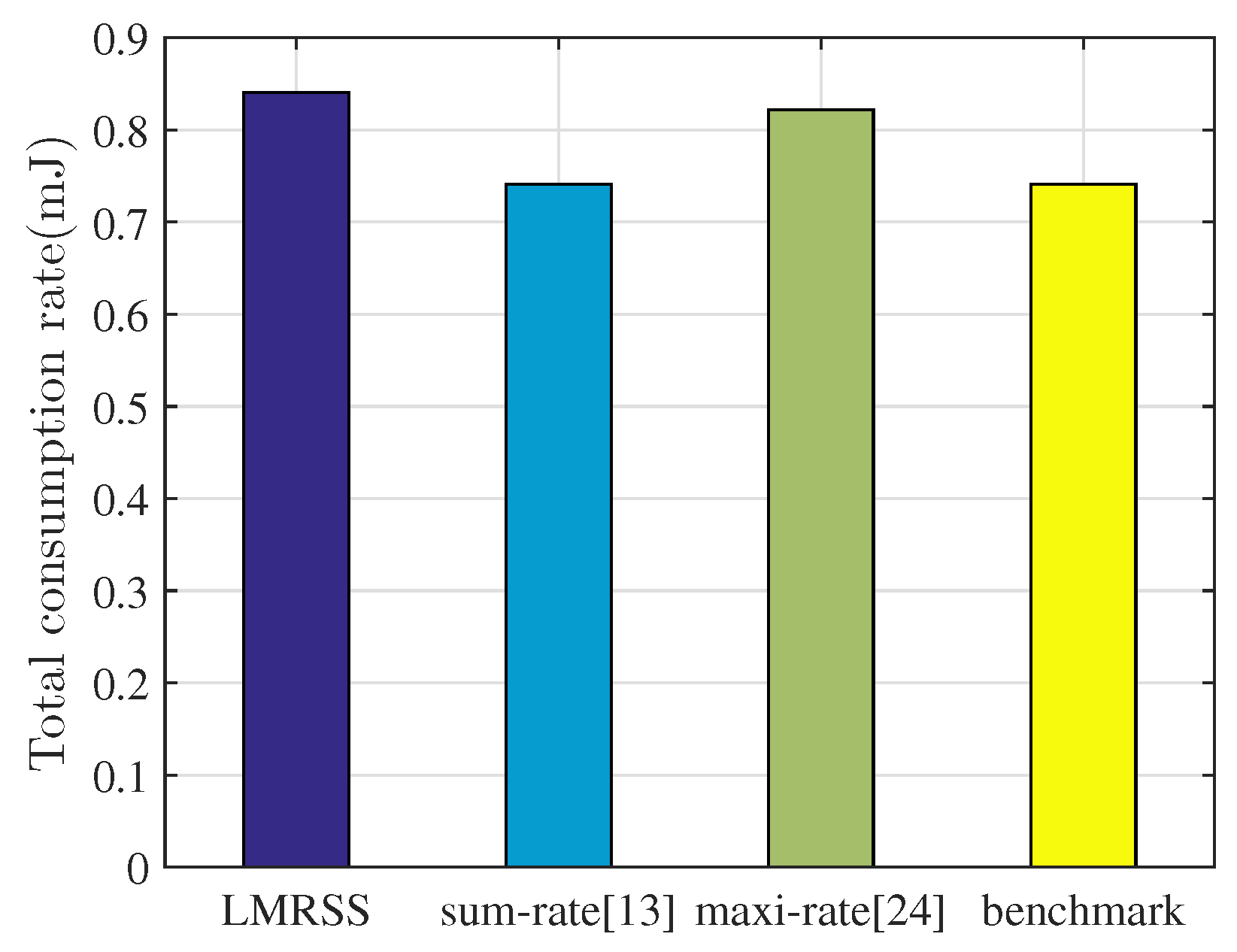
Figure 4 shows the averaged sum of energy consumption rates of sensor nodes in one superframe under different relay selection algorithms in the simulation. It can be seen that the sum-rate algorithm together with benchmark spends the least because of its optimization objective. LMRSS consumes 13% and 5% more energy than the sum-rate algorithm and maxi-rate algorithm, respectively. It is inferred from the figure that the sum-rate scheme realizes the best energy efficiency, which is the minimum sum of energy consumption rate of all of the sensor nodes in the network, but it does not get the best performance of enhancing network lifetime. Hence, just concentrating on network level energy efficiency is not an appropriate way to prolong network lifetime, as shown in
Figure 3. More specifically, in the environment of WBANs, where lifetime may be more important than energy efficiency, LMRSS results in a slight drop in energy efficiency; however, it produces more considerable improvement of network lifetime.
In addition to the explanation for the impact of energy consumption and energy storage of sensor nodes on network lifetime performance, we analyze the worst case for relay selection where sensor nodes in the main body part possess less energy than other nodes in the rest parts. That is, relay nodes are short of energy more seriously than faraway sensor nodes. In this case, LMRSS is out of action since it aims to protect relay nodes that are more energy-restrictive and may run out of energy first. In order to prolong the lifetime of relay nodes, LMRSS will not allocate faraway sensor nodes to any relay nodes so as to cut down on the energy depletion of relay nodes. As a consequence, LMRSS is equal to the direct transmission strategy in this case. On the contrary, the maxi-rate algorithm focuses only on energy consumption of WBANs, and it will still allocate faraway sensor nodes to energy-restrictive relay nodes to achieve its target on energy consumption rate. As a result, relay nodes will accelerate to exhaustion, which, in turn, degrades the network lifetime performance of WBANs.
Table 4 shows the network performances of different relay selection methods in the worst case via simulations to validate our analysis above. We set residual energy in sensor nodes belonging to the main body part as 1 J and as 2 J for the other sensor nodes in the network to simulate the worst case in relay selection. As shown in the table, for the maxi-rate algorithm, the maximum consumption rate of sensor nodes within the networks is the lowest. However, its network lifetime performance is decreased by 30% compared with the benchmark strategy since the maxi-rate algorithm only focuses on the energy consumption criterion and neglect energy storage of each sensor node. Meanwhile, as discussed before, LMRSS in this case selects to use direct transmission only, which is the same with benchmark strategy.
As stated in
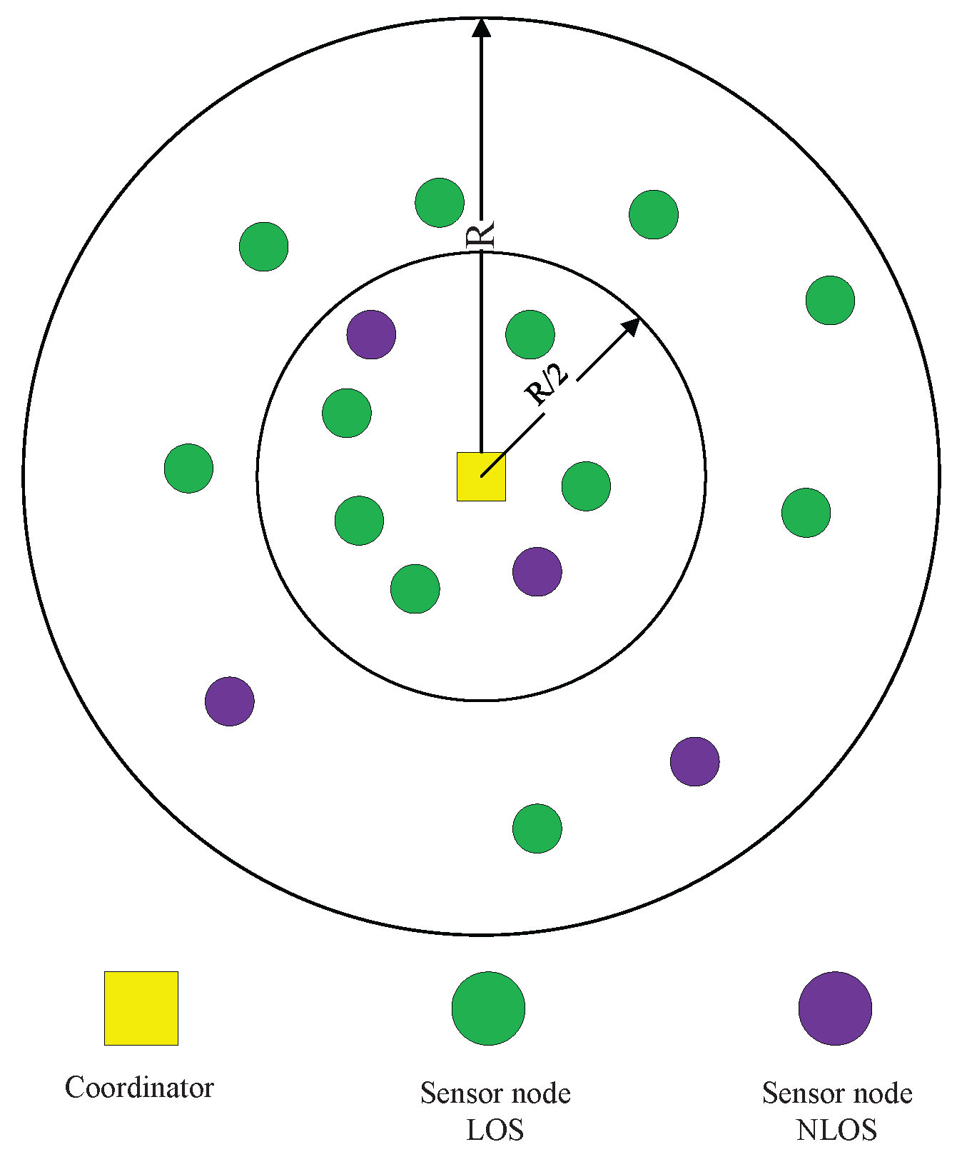
Section 1, WBANs are not only specified to be used on the human body. For example, in interactive gaming, robots whose shapes are not restricted to the human form but also tree-form or ball-shaped will also need deploying WBANs to fulfill their mission in the game. Therefore, in this paper, we design a more general WBAN model according to IEEE 802.15.6 to comprehensively evaluate our proposed algorithm. In this standard, the typical network range is regulated to be less than 3 m and the maximum number of nodes in a WBAN is up to 64. The designed model is illustrated in
Figure 5. In the figure, the coordinator is placed in the center of a circle whose radius is
R while sensor nodes are randomly placed in the area of the circle. When the distance of a sensor node from the coordinator is less than
, it is treated as a candidate relay node, which, in the figure, is deployed in the circle with the radius of
.
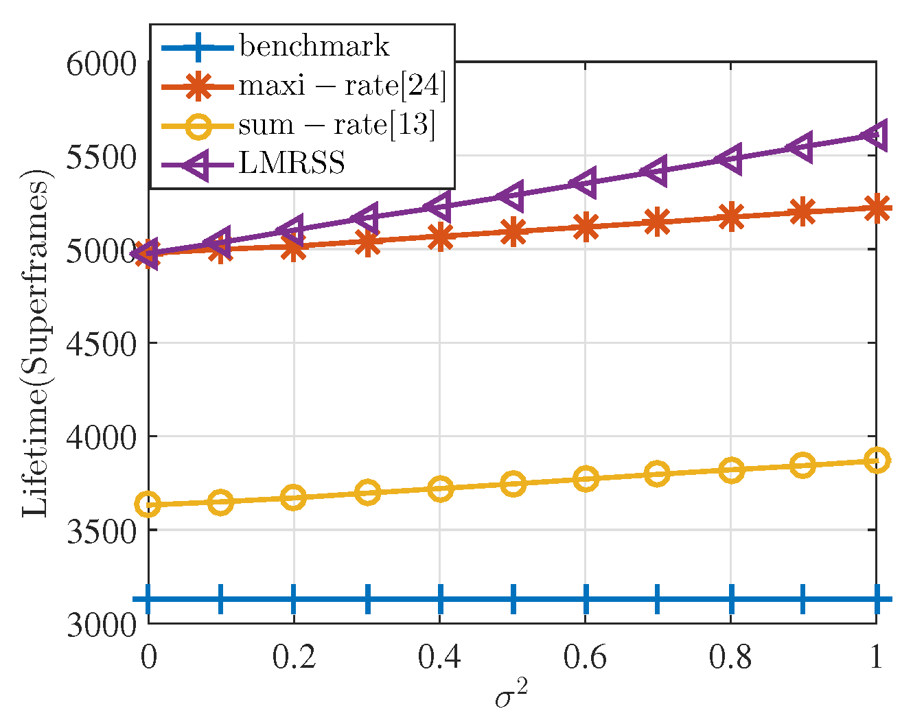
Figure 6 shows the lifetime performance with the variation of
on the aforementioned WBAN general model. The
R is set to be 3 m, and the number of nodes is 16 in the simulation. It is illustrated that the proposed algorithm outperforms the other three. In more detail, when
, the proposed algorithm improves network lifetime by 59%, 37%, and 0% compared with benchmark, sum-rate algorithm and maxi-rate algorithm, and gradually increases to 79.2%, 45% and 7.4% when
increases from 0 to 1. The increasing gaps result from the fact that the proposed algorithm considers the residual energy condition of each node as well as the consumption rate. It is also noticed that the performance of the sum-rate algorithm is not the same as the benchmark, which is different from the model in
Figure 1. This is because the distance in this model is larger, and two-hop transmission can be selected in certain conditions to effectively reduce the transmission energy for some far-away nodes, resulting in a decrease of the total network energy consumption.
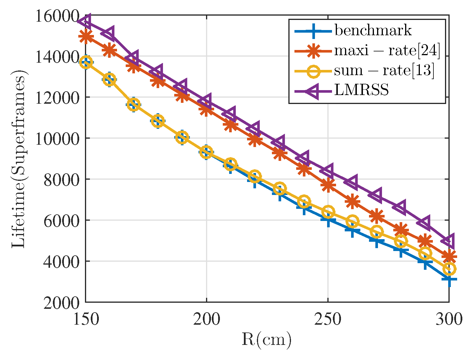
Figure 7 shows the lifetime performance with the variation of
R. The number of nodes is still 16 and the
is set to be 0.5 in the simulation. It is indicated from the figure that the proposed algorithm still has the best performance no matter how
R varies. The performance of the sum-rate algorithm is the same as the benchmark when
R is small and becomes better if
R is larger than 2 m. LMRSS improves network lifetime by 14% compared with the benchmark and sum-rate algorithm and increases to 59% and 37%, respectively, when
R is 3 m. Furthermore, when compared with the maxi-rate algorithm, the performance enhancement increases from 4.6% to 18% if the distance varies from 150 cm to 300 cm. It is true from the results that the advantage gap of LMRSS over the other three becomes larger with the increasing value of
R. The reason for this phenomenon is that with the growing network range, two-hop transmission brings about more transmission distance reduction, which leads to more transmission energy saving. Therefore, the impact of cooperative transmission and its relay selection on network lifetime becomes more and more significant.
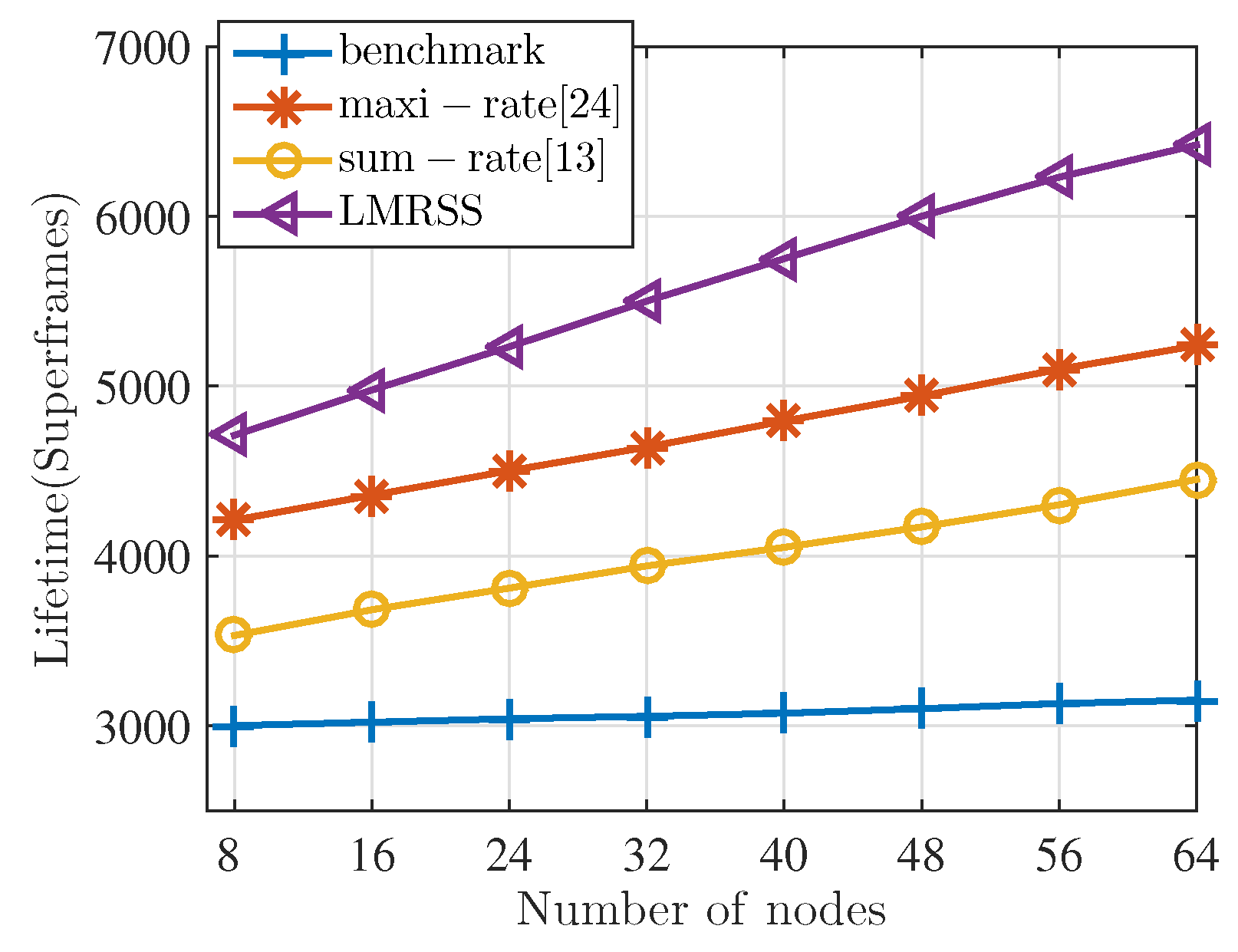
Figure 8 shows the lifetime performance under different total numbers of sensor nodes in WBANs.
R is set to be 3 m and the
is set to be 0.5 in this scenario. It can be seen from the figure that, except for the benchmark, which only utilizes direct one-hop transmission to communicate, the other three relay selection schemes will perform better if the total number of sensor nodes increases. The reason for this observation is that more sensor nodes in the network will provide more choices of relay nodes for the sensor nodes, which need two-hop cooperative transmission. As a result, relay selection schemes can allocate more appropriate relay selection to each sensor node in WBANs, which, in turn, prolongs the network lifetime. Furthermore, in the figure, LMRSS outperforms other schemes and the gap between LMRSS and the other two scheme becomes larger with the increasing number of nodes. In particular, the gap between LMRSS and benchmark varies from 57% to 103%, 33.4% to 44.3% for the sum-rate algorithm, and 12% to 22.4% for the maxi-rate algorithm.
To conclude the simulation results presented above, the advantages of LMRSS can be summarized as follows:
In a body-shaped WBAN application scenario, the proposed scheme can effectively improve the network lifetime of WBANs by 11.8% at least when compared with the direct transmission strategy and is also proved to be better than other existing relay selection methods. A comprehensive comparison between LMRSS, maxi-rate algorithm and sum-rate algorithm is summarized in
Table 5 based on the simulation results.
As LMRSS takes battery capacity diversity into account, it selects relay nodes depending on not only the energy consumption condition but also the remaining energy of each sensor node. When serious energy inequality conditions appear in the network, the advantage of network lifetime improvement of LMRSS is more significant when compared with other schemes.
The network lifetime advantage of the proposed LMRSS is not restricted in body-shaped WBAN applications. As in a more generalized WBAN model, which is specified in the IEEE 802.15.6 standard, LMRSS still performs better than direct transmission and other existing relay selection methods in terms of network lifetime, no matter how the factors (energy inequality degree, range, number of nodes) vary.
The time complexity of LMRSS is low, which can be implemented in a real-time WBAN system.
6.3. Implementation Discussion
In addition to the performance evaluation of our proposed relay selection scheme through simulations, in this part, we make a brief introduction to how to implement our relay selection scheme in a real WBAN system so as to validate the feasibility of the proposed scheme.
We firstly list the parameters needed to execute our relay selection scheme and describe the methods to obtain the values of these parameters:
: the distance between each pair of sensor nodes and the distance between sensor nodes and the coordinator;
n : the transmission path state (LOS/NLOS) between each pair of nodes including the coordinator;
: the energy consumption parameters;
k: the packet length in the network;
: the energy storage condition of each sensor node in the network.
As the total number of sensor nodes in a WBAN is not large, can be measured manually after the sensor nodes have been deployed as well as n, e.g., the transmission path state of each pair of nodes according to the location of each node. Furthermore, the energy consumption parameters are obtained depending on the transceiver types of sensor nodes in the networks. k is specified by the communication protocol and is easily known by WBAN users. can be known by two means depending on two conditions: (A) if the relay selection is invoked at the network initialization where each sensor node is full of energy, we can directly obtain the energy storage information from the sensor node type and battery information; (B) if the relay selection is invoked at a restart from a network recovery, the coordinator can set a request flag in the beacon frame in order to inform each sensor node to report its residual energy condition in the following transmitting time slots. When all of the above parameter values are obtained, the coordinator records this information in its memory and has the ability to execute the relay selection scheme.
Then, we illustrate how to implement our relay selection scheme in two cases. In the first case where a WBAN is at the initialization stage, the coordinator will directly execute the relay selection scheme at the beginning of the first superframe since it has all values needed to execute the relay selection scheme and load the relay allocation results and the corresponding timeslot allocation in the beacon frame. Then, in the beacon transmission slot, the coordinator broadcasts the beacon frame to all of the sensor nodes in the network. As each node must listen and receive this beacon frame, all of the sensor nodes in the network will know their transmission strategy and their relay nodes, if needed.
In the second case, e.g., a WBAN restarts, where the energy storage condition of sensor nodes is unknown, the coordinator sets a request flag in beacon frame at the beginning of the first superframe and allocates timeslots for each sensor node in the network to report their energy storage conditions. As a result, in the first superframe, sensor nodes send their energy storage information to the coordinator in their allocated report slots. After the coordinators have received all of the report frames, it invokes the proposed relay selection scheme and loads the results and the corresponding timeslot allocation in the next beacon frame, which will be broadcasted in the second superframe. Then, in the second superframe, each node will know its transmission strategy and their relay nodes.
It should be emphasized that the low complexity of the rapid solution in our proposed scheme guarantees that the coordinator can finish the algorithm in the interval between the point when the coordinator has received all the energy storage reports to the slot for broadcasting the next beacon frame. Furthermore, it should be noticed that the implementation discussed here does not involve the detailed interaction procedures between the coordinator and sensor nodes that will be further studied in the future.


