
Consensus-Based Cooperative Control Based on Pollution Sensing and Traffic Information for Urban Traffic Networks


Centre for Automation and Robotics (CSIC—UPM), Ctra. Campo Real Km. 0.2, Arganda del Rey, 28500 Madrid, Spain
*
Author to whom correspondence should be addressed.
Sensors 2017, 17(5), 953; https://doi.org/10.3390/s17050953
Submission received: 6 February 2017
/
Revised: 30 March 2017
/
Accepted: 21 April 2017
/
Published: 26 April 2017
(This article belongs to the Special Issue Selected Papers from the 3rd International Electronic Conference on Sensors and Applications)
Abstract
:Nowadays many studies are being conducted to develop solutions for improving the performance of urban traffic networks. One of the main challenges is the necessary cooperation among different entities such as vehicles or infrastructure systems and how to exploit the information available through networks of sensors deployed as infrastructures for smart cities. In this work an algorithm for cooperative control of urban subsystems is proposed to provide a solution for mobility problems in cities. The interconnected traffic lights controller (TLC) network adapts traffic lights cycles, based on traffic and air pollution sensory information, in order to improve the performance of urban traffic networks. The presence of air pollution in cities is not only caused by road traffic but there are other pollution sources that contribute to increase or decrease the pollution level. Due to the distributed and heterogeneous nature of the different components involved, a system of systems engineering approach is applied to design a consensus-based control algorithm. The designed control strategy contains a consensus-based component that uses the information shared in the network for reaching a consensus in the state of TLC network components. Discrete event systems specification is applied for modelling and simulation. The proposed solution is assessed by simulation studies with very promising results to deal with simultaneous responses to both pollution levels and traffic flows in urban traffic networks.
1. Introduction
Nowadays, the challenge of making sustainable and environmentally friendly cities is driving the activities of many stakeholders such as local and national authorities, the private sector, environmental pressure groups, university research institutes, and neighborhood associations. They are jointly promoting system-of-systems-based solutions for smart cities [1,2,3]. From a physical and system engineering standpoint, a city or an urban region can be considered as a physical system composed of several coupled physical subsystems with thousands of networked sensors and actuators (e.g., transportation, energy distribution systems, water supply systems, etc.). Thereby, the overall dynamic performance of the city can be assessed on the basis of the emerging behavior of these coupled physical subsystems having three important features: complexity, uncertainty and heterogeneity. Strict requirements for sustainability, resource availability, and optimality are then imposed. The ability to anticipate and control daily situations (e.g., traffic congestion and high levels of pollution) and unexpected events (e.g., power failures, traffic accidents and exceptional climate conditions) is a key issue to deal with complex and potentially unstable conditions. In addition, many sensors, actuators, communication systems, and computing platforms are available in each subsystem. Therefore, the development of integrated methods based on these sensory data, signal processing strategies and decision-making procedures is a challenge with no straightforward mathematical tractability, and difficult representation and evaluation by traditional modeling and simulation tools. New computing platforms are able to measure representative variables, perceive physical events that may occur in the environment, preprocess the events with embedded computing capabilities and send information to networked and distributed applications that can perform more complex tasks for managing complete urban systems.
Current research on smart cities aims to integrate urban subsystems [3]. These subsystems are usually from different domains or with different timing and bandwidths. Two examples are the pollution measurement systems and the traffic control and monitoring systems. The heterogeneity of the systems imposes new challenges in model-based design approaches. On the other hand, the increasing number of sensors, actuators, communication systems and computing devices already deployed in cities, enable new applications to go beyond particular solutions and cover wider urban systems and scenarios. These challenges have been recently addressed in other application fields by using machine learning techniques, data mining or artificial cognition-based strategies [4,5].
The System-of-Systems (SoS) paradigm emerges from the need to address the complexity of interconnected systems. In this context, systems are independently designed, evolve independently and can operate autonomously [6,7]. Nevertheless, the constituent systems of a SoS have their own individual goals while the whole SoS has global goals. The expected goal of operating sub-systems that work together is a better overall yield of the sum of the systems in comparison with each individual system. Their joint operation provides new functionalities; subsystems are also operationally independent and autonomous, so interactions between them are generally asynchronous and can be represented as discrete-event models [8]. This heterogeneity of the systems brings new challenges to the model-based design approach.
How can cooperative control and sensing systems be designed on the basis of SoS paradigm to provide new sensor-based solutions for smart urban systems?
The design of cooperative control strategies for urban subsystems can be supported on centralized and distributed coordination schemes [9]. In a centralized coordination scheme, it is assumed that each system has the ability to communicate with a central unit or share information via a fully connected network. On the contrary, distributed coordination schemes reduce communication requirements using local neighbor-to-neighbor interactions, thus improving scalability, flexibility, reliability and robustness.
Consensus is a fundamental issue to be considered for designing cooperative control for distributed multi-agents coordination. Some reports on cooperative control of sets of multiple subsystems such as vehicles, robots and rovers are inspired in consensus-based approaches [10]. Nanayakkara et al. [8], suggested a consensus-based control using the cooperative-control paradigm, to increase the expected benefits of the resulting system. These authors proposed to create a set of systems each pursuing its own objectives as well as their common goals, using communications between subsystems.
Consensus algorithms have been widely applied to distributed cooperative systems such as vehicle groups [9,11,12], swarm robots [10], traffic control systems [13,14,15], traffic speed density prediction [16] and wireless-sensor networks [17], among others. In these cases, consensus control enables each individual system or agent to ascertain the global goal and then, based on the state of the other system, to make decision on the best control signal to achieve the corresponding goal.
The problem of traffic optimization in urban environments based on city-pollution information can be addressed by a consensus-based approach between different control agents [18]. Focused on a similar problem (urban-traffic management and control), Castro et al. proposed a multilayer distributed model for predictive control of urban traffic. The control system was composed of local and global layers of controls where each control agent is responsible for traffic lights at one intersection. The system uses the principles of consensus between control agents and behavioral coordination, in order to conciliate local and global control objectives.
In another work reported in [19], the distributed control principle was applied to a network of intersections, with the aim of controlling the traffic at a macroscopic level. Wuthishuwong et al. implemented a discrete time-consensus algorithm, to coordinate the gross traffic density of an intersection and its neighborhoods in the network. The traffic density at each intersection was collected, by using Vehicle-to-Infrastructure (V2I) communication, and the information was distributed to the neighborhood via Infrastructure-to-Infrastructure (I2I) communication link. Each intersection performed as a centralized controller that computed the control signal using both, own and neighborhood information on traffic density. Intersections were considered individual nodes, in order to apply the consensus strategy, and each node shared information on its traffic density and coordination variables.
In this work, the System-of-Systems (SoS) engineering paradigm sets the foundation for developing a cooperative control strategy applied to an urban scenario. For this purpose, the air-pollution information service and the traffic control subsystem are put together, and the control system makes use of available information to modify or adjust traffic-light cycles at intersections. Due to the distributed nature of the main subsystems, a distributed consensus-based control method is developed. Pollution levels and traffic densities are considered inputs of the proposed control strategy based on subsystems cooperation. It should be noted that sources of air pollution in cities are not only coming from vehicle emissions but also from industrial activity, domestic fuel burning, boilers for heating, etc.; which increases the complexity for considering the whole problem. Modeling and simulation are not straightforward according to the complexity of main subsystems, instead both can be powerful tools to address the problem and generate the basic knowledge on this field. The discrete event systems specification (DEVS) is applied for modeling and simulation in this work. The main rationale for using DEVS relies on the suitability of this framework for modeling complex dynamical systems and their interactions [20].
From the best of authors’ knowledge the main contribution of this work is the design and evaluation of a strategy for improving the performance of urban traffic networks in specific regions of a city taking into account traffic and pollution sensory information. A consensus-based cooperative control method is proposed by taking advantage of new developments on technologies and concepts for smart cities. This paper is organized as follows: in Section 2, a brief review of pollution and traffic sensing systems is presented. Section 3 introduces the problem and the proposed solution. Section 3.1 deals with the modeling technique for representing the behavior of the main subsystems components. Section 3.2 addresses the consensus-based cooperative control and presents the proposed cooperative control solution. Section 3.3 and Section 3.4 show open-loop and closed-loop simulation results. Discussions on the main results are given in Section 4. Finally, the conclusions are presented in Section 5.
2. Review of Pollution and Traffic Sensing Systems
In the last years, the interest in collecting data in cities has increased substantially. The current trend is to make a better use of public resources while increasing the quality of the services that citizens can access [21]. In particular, urban air quality sensing and traffic information are attracting a lot of research because of growing population in cities. In this section, a brief review about pollution and traffic sensing systems in cities is presented.
2.1. Pollution Sensing Systems
The basis for the consensus-based cooperative control is the pollution sensing system. Current sensors for pollution concentration measurement are based on different chemical of physical principles such as chemoresistance, solid electrolyte, absorption, etc. These sensors can measure different pollutants such as O2, O3, CO, carbon dioxide (CO2), mono-nitrogen oxides (NOx), PM, and volatile organic compounds (VOCs), in different range of sensitivity, selectivity and response time. Depending on the application, the sensor can be chosen with the required specific parameters e.g., in [22] an O2 with a sampling time of 1.6 s and NO2 with a sampling time of 41 s are selected.
Traditional approaches for pollution monitoring in urban or rural areas are based on networks of fixed stations for measuring air quality. Typically, these networks can provide detailed data but limited to the location of the stations. This makes that modelling approaches are usually used for obtaining representative pollution information in the area of interest [23].
The current challenges in the assessment of human exposure to pollution are how to make available reliable pollution data in cities, and how to handle large amounts of data from high resolution sensors and process it. Most recent methods propose the deployment of low-cost sensors that can provide emission information that allows the development of mitigation strategies [23]. In contrast with traditional approaches, the advances in sensor compactness, robustness, and wireless communications let sensor networks to be remotely managed, to easily transmit collected data and to report high spatial-resolution information in near-real time [24]. Data from these new pollution information systems enable a better pollution assessment and the development of new control strategies for pollution reduction [23].
2.2. Traffic Sensing Systems
The performance and safety of traffic control and management systems depend directly on traffic sensing systems. As in the case of pollution sensing systems, in the last decade there has been significant progress in the application of computer, sensing and communication technologies to traffic management and sensing systems [25]. Nowadays, there exist different technologies for traffic sensing that are suitable for several scenarios depending on the installation of the sensors, maintenance, performance, atmospheric conditions, etc. Some of them are: inductive loops, radio-frequency identification (RFID), microwave radar, acoustic, magnetic, ultrasonic and video image processor (VIP) [25]. Inductive loop detectors are commonly used for traffic sensing in cities and highways due to their characteristics: they are suitable for different weather conditions and different traffic volumes [26]. They also provide consistent and accurate measurements. Induction loops are also capable of measuring vehicle speed and vehicle classification, what make them appropriate and reliable for provide data to traffic control systems [27].
3. General Scenario and the Proposed Solution
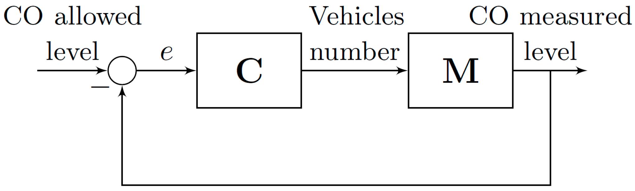
We have defined a general scenario based on a smart mobility application with the aim of improving the performance of urban traffic networks in urban regions of a city. The scenario is based on an emission control scheme proposed by Andò et al. [28]. These authors suggested the idea of a vehicles emission control scheme for traffic flow control as a possible solution to address the problem of urban air quality (see Figure 1). However, they do not provide specific solution for designing the emission controller. Authors proposed the number of allowed vehicles as the main control signal whereas the difference between the innocuous allowed CO level and the CO measured level is the input signal.
A new control scheme and a procedure that can be integrated into the Adaptive Traffic Control System (ATCS) of an urban area are proposed in this work [29]. The ATCS adjusts, in real time, signal timing plans based on the current traffic conditions, demand, system capacity, among other conditions. In the control scheme suggested in this work, we focused on designing the adaptive component for traffic lights cycles . The traffic lights cycles can vary on the basis of the following relationship , where is the value set by other components of the ATCS or by traffic engineers.
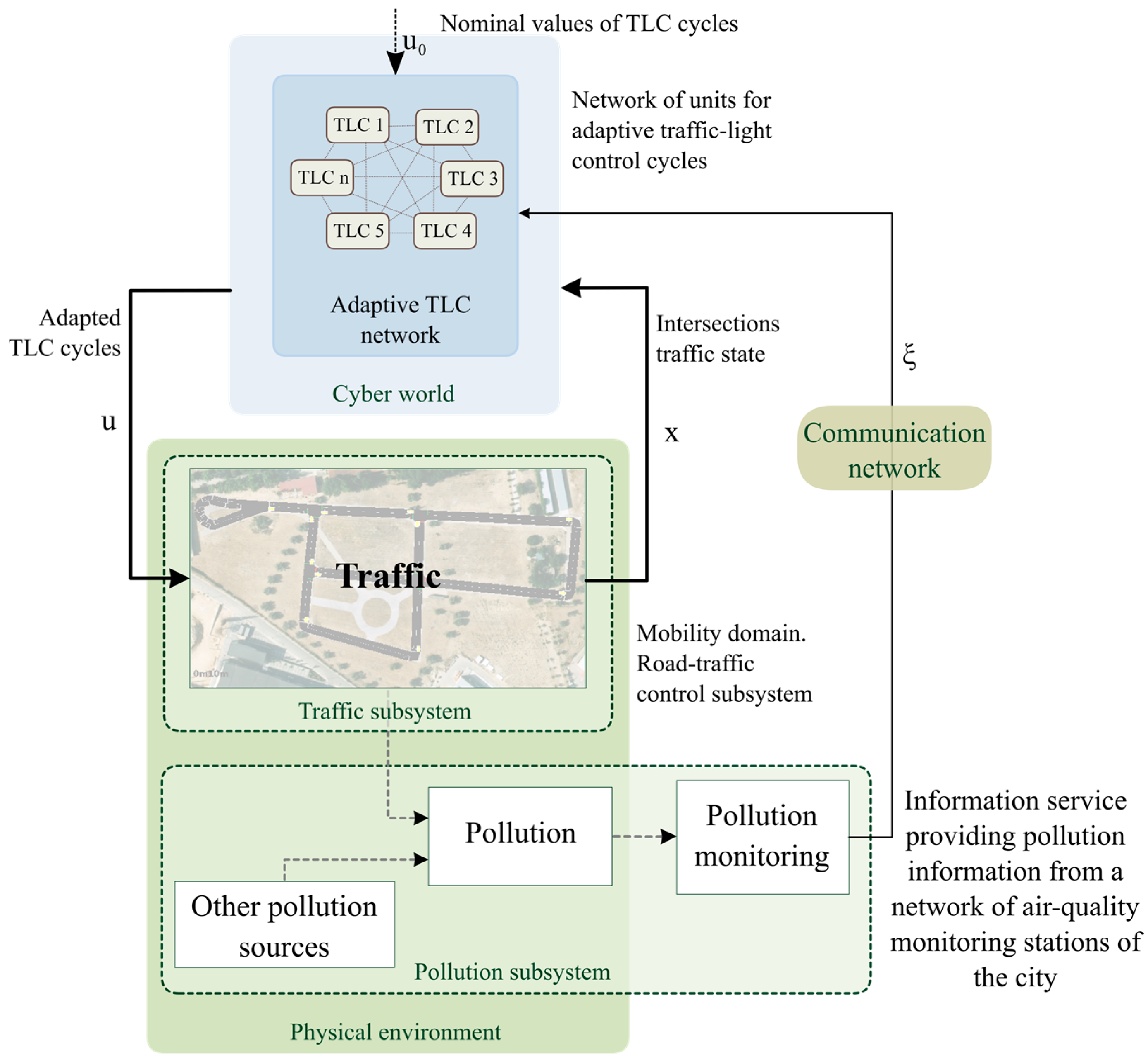
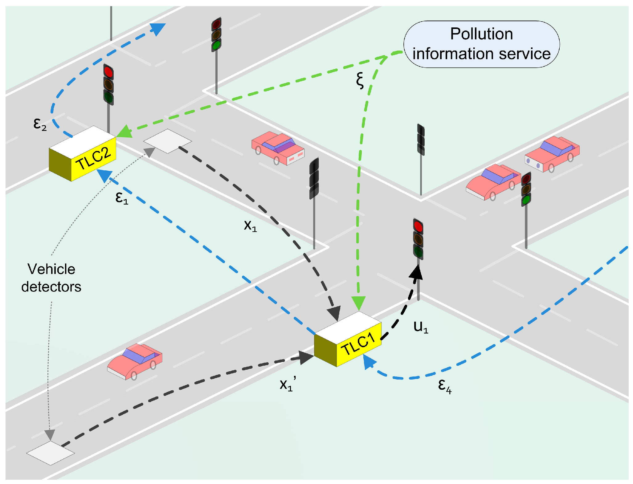
Figure 2 depicts a general diagram of the scenario and the strategy proposed in this work. Interconnected traffic lights control (TLC) network adapts the traffic-light cycles based on air pollution data provided by the city information service and local traffic measurements. The air pollution information service provides data () from the city pollution sensing system. Moreover, traffic information () is given by the vehicle detection sensor placed at each intersection of the urban traffic network. The traffic lights cycles () are updated by TLC units which make decisions based on a consensus variable () derived from the consensus-based control method.
The following subsections address the modeling, control design, and simulation of the whole system.
3.1. Modeling
In order to study the dynamic behaviour and the interaction between the different components of the scenario, Discrete Event Systems Specification (DEVS) formalism is selected as a framework for SoS modeling and simulation. This formalism can be used for modeling and simulating complex dynamical systems and their interactions [20]. The DEVS modeling-based approach enables specification of basic models and how they are connected together. These basic models, known as atomic models, are modular systems with inputs (through input ports), changing states, and outputs (through output ports) running in a time frame. The couplings between atomic models generate coupled models.
In this work we used Parallel DEVS formalism (PDEVS) which solves collisions between internal and external transitions allowing all components to be activated and to send their output to other components. A basic PDEVS model can be represented as:
where,
- is the set of input ports (p) and values (v)
- is the set of output ports (p) and values (v)
- is the set of states
- is the internal transition function
- is the external transition function
- is the confluent transition function
- is the total state set and e is the time since the previous transition
- is the output function
- is the time advance function
Basic PDEVS models have a bag of inputs. A bag is a set with possible multiple occurrences of its elements e.g., {a,b,a,c} [30]. PDEVS also introduces the confluent transition function (), which decides the next state in case of collision between external and internal events () without the need for a priority scheme. This option provides a complete control over the collision behavior. Instead of serializing model behavior through the select function at the coupled-model level, PDEVS leaves this decision to the individual component. After modeling, it is necessary to conduct simulation studies. DEVS simulation methods generate the corresponding behaviors of each model, which are trajectories that can even reach illegal states by following execution protocols. This modeling paradigm serves to represent each subsystem as an atomic model that can be coupled with other model, forming coupled models.
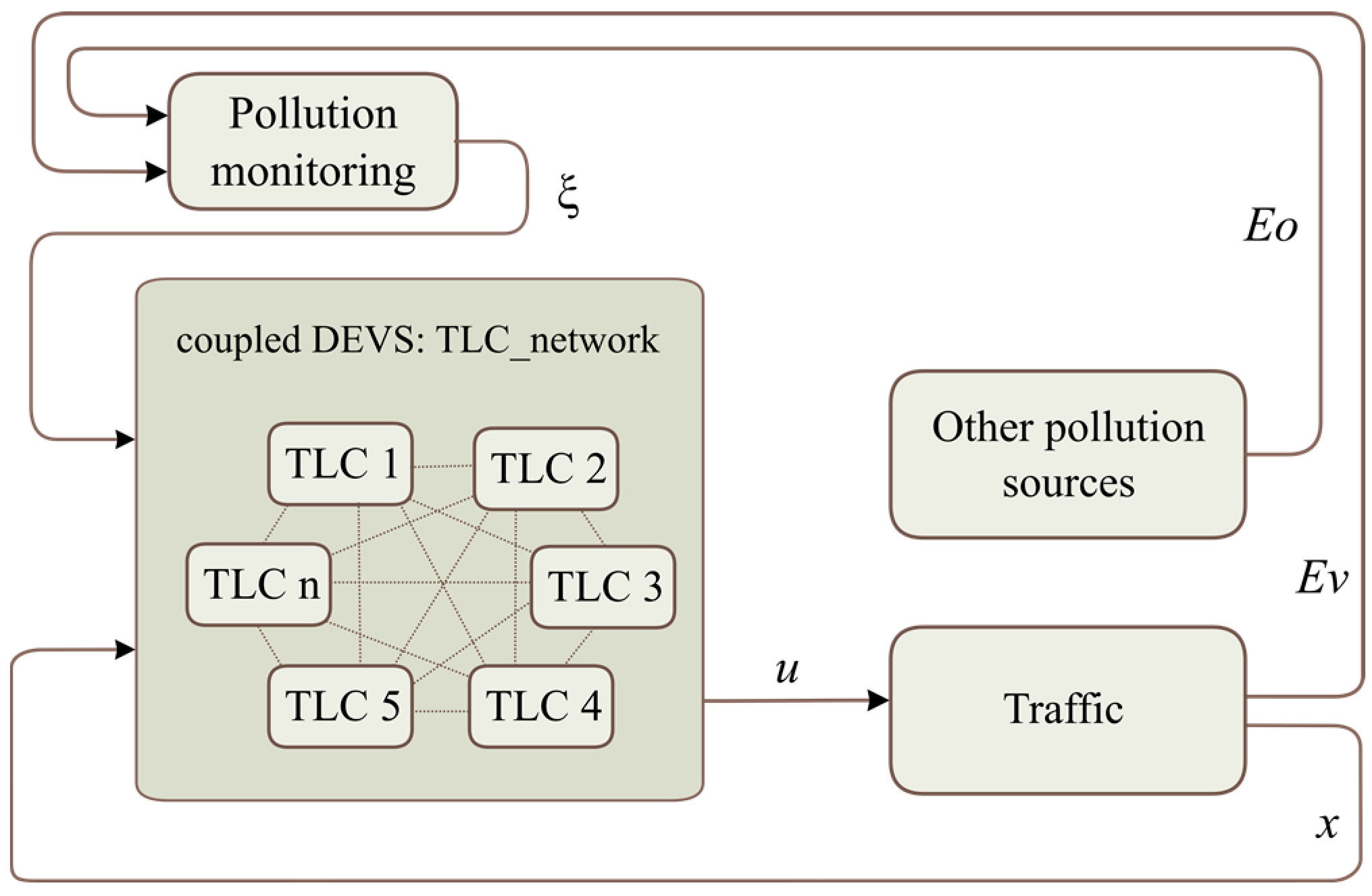
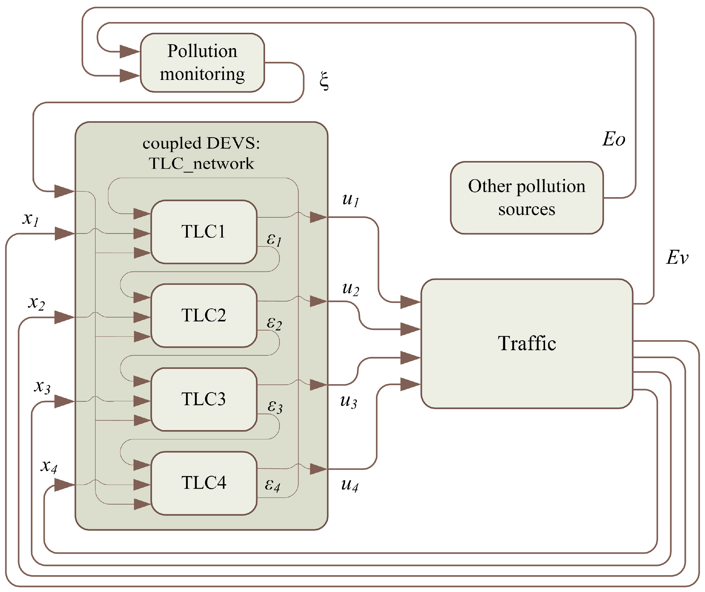
This section addresses the representation of the system based on a conceptual model and the data flows between subsystems. Every system is represented as an atomic discrete system. The coupling of atomic models forms a coupled model. Figure 3 depicts the structure of a DEVS model of the general scenario and how the subsystems are connected.
In the above model, the following systems are defined as atomic models:
- Traffic-light control unit (TLC)
- Pollution-monitoring service
- Traffic system (i.e., road network, vehicles, traffic lights, etc.)
- Other pollution sources
The network of interconnected TLCs shares information (consensus variable, ) to achieve a consensus between each other. This network is modeled as a coupled model. Each TLC is connected with a Traffic system to adapt the cycle length () of the corresponding traffic lights. The output of the Traffic subsystem is the traffic information (i.e., traffic flow at every intersection, ) and the pollution data from urban road traffic (Ev). The system called “Other pollution sources” emulated the pollution contribution of other urban subsystems (e.g., building heating systems, other transportation systems, etc., Eo). The Pollution monitoring system is represented by the urban pollution-measurement system that brings information on air quality to the TLC network (). Data flows illustrated in Figure 2 and Figure 3 are summarized in Table 1.
3.2. Consensus-Based Cooperative Control Design
Consensus algorithms are thought to be distributed algorithms that assume only neighbor-to-neighbor interactions between subsystems. Subsystems update their information states based on their neighbors. The aim is to design a control strategy for updating the information states of all of the subsystems in the network, so that they converge to a common value.
The main rationale of a consensus-based procedure is to impose similar dynamics on the information states of each subsystem of the network [9]. Depending on the typology of the network for connecting subsystems, two different approaches can be applied. Firstly, if the network allows continuous communication, then the information state is modeled using differential equations. Secondly, if the data are communicated through discrete packets, the information state is represented by difference equations.
The topology for interactions in a network of agents is represented using a graph , where is a finite none-empty node set and is an edge set of ordered nodal pairs, called edge. The edge (i, j) in the edge set of a graph denotes that node j can obtain information from node i. The neighbors of a node i are denoted by . An iterative form of the consensus algorithm to reach an agreement in relation to the state of n integrator nodes with dynamics can be represented in discrete time as follows:
where, is the entry in row i and column j of the adjacency matrix associated with , and is the information state of the i-th system. A consequence of this equation is that the information state of the system i is driven toward the information states of its neighbors. The consensus is achieved if, for all and for all , , as .
The procedure to apply the consensus-based control and the results are then presented. The goal of the control system is to achieve a consensus between the intersections related to an estimation of local emissions (consensus state variable) by adapting local traffic-light cycles. The consensus-based decision-making takes into consideration the air-pollution state, provided by the air pollution information service, and the local traffic state. Specifically, a discrete consensus-based control algorithm is applied to control the coordination of the TLC network. The main steps for designing the control system are described in the following subsections.
3.2.1. System Dynamics
A consensus variable that represents the system dynamics should be defined. Each TLC uses local traffic and pollution sensing information from a pollution information service. Therefore, an estimation of the pollutant concentration at each intersection as the consensus state variable is taken. The dynamics of each intersection is the same and it is assumed to behave as a local linear system. The discrete dynamic model of the node, that includes traffic information and pollution sensing data, is defined by the following recursive equation:
where,
- [gNOx/m3] is the state of the system at instant . The state of the system is related to the pollution levels and the traffic state at each intersection. The pollutant considered in this study is NOx (mononitrogen oxides).
- [gNOx/m3] is a system input. It contains the pollution information provided to the TLCs at instant where is the delay between pollution production and pollution information reception by the TLCs.
- is a dimensionless parameter that represents the contribution of intersection to overall city pollution. It is computed on the basis of the maximum occupancy of intersection over the total maximum occupancy.
- [veh] is a system input. It contains the summation of vehicle queues at every approach of the intersection controlled by TLCi. represents the delay between traffic queue measurement and traffic information reception at TLCi.
- [gNOx/veh/m3] is the pollutant emissions of a given traffic queue at an intersection. , where is the emission factor of the pollutant (gNOx/veh/km), is the dispersion factor of the pollutants (s/m2) and is the simulation step [31].
- [% T.L. cycle] is the consensus-based cooperative control output of TLCi. The control signal is a percentage change of the cycle length of the traffic lights with respect to the initial cycle length in a limited range. This component is defined later (control law design).
- [gNOx/m3/% T.L. cycle] represents the influence of the pollutant emissions on traffic-light timing. , where [veh/% T.L. cycle] is a parameter that represents the queue length with respect to changes in traffic-light cycle lengths. Therefore there is a proportional relationship between and .
3.2.2. Design of a Consensus-Based Control Strategy
The control strategy adopted for each TLC (nodes of the network) makes use of pollution and traffic information as well as information from neighbors. Taking into account the dynamic model considered in (2) and applying the consensus control described in (1), the control strategy is represented by:
where,
- is a parameter that refers to system stability. If , where is the maximum degree of the graph, consensus convergence is guaranteed in a connected graph [32].
- is the corresponding value of the adjacency matrix.
This control law contains three components, shown in Table 2.
In order to avoid large dissimilarities with the original traffic-light cycle lengths, the values of the control input are constrained to a variation of ±50% over the initial value.
3.3. Open-Loop Simulation for Test Scenario: Pollution and Traffic-Based Control Are Switched Off
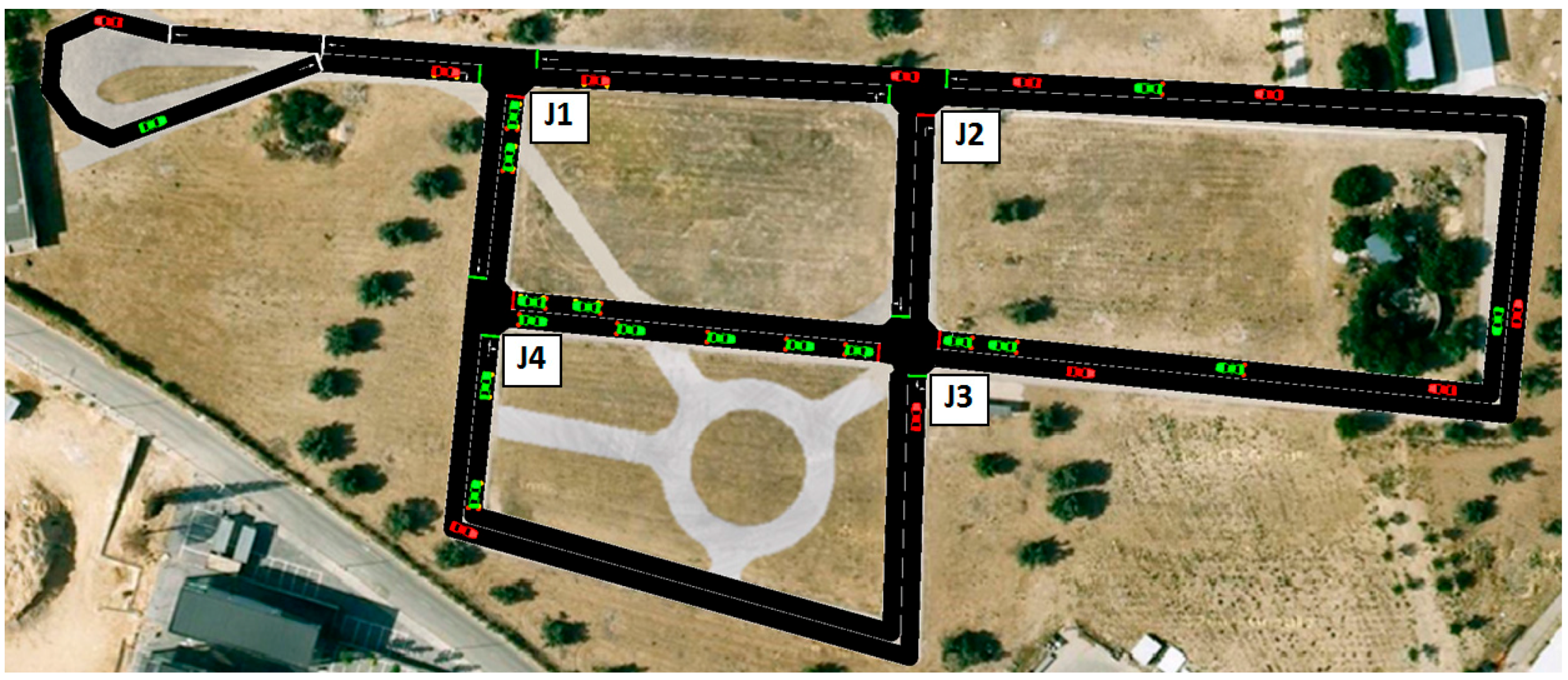
The scenario is based on an urban-like road network depicted in Figure 4. In order to simplify the description of the proposed solution, we considered a test scenario composed of four signalized traffic intersections (junctions J1, J2, J3 and J4) and interconnected TLCs. Vehicles are moving on the road network, following predefined routes randomly generated for imitating urban traffic. The vehicles included in the scenario are of the same type and use the same car-following model which is a version of the model defined by Krauß et al. [33]. In this version, different deceleration capabilities of the vehicles are handled without violating safety (the original model allowed for collisions in this case), and the formula for safe velocity is adapted to maintain safety when using the current Euler-position update rule. The parameters defined for vehicles and the car-following model are shown in Table 3.
The number of trips is defined by the repetition rate (number of trips per second). The repetition rate is calculated randomly by using a normal distribution with a mean of 5 and standard deviation of 0.25. Routes were generated, ensuring a minimum straight-line distance between the start and the end edges of a 170-m trip.
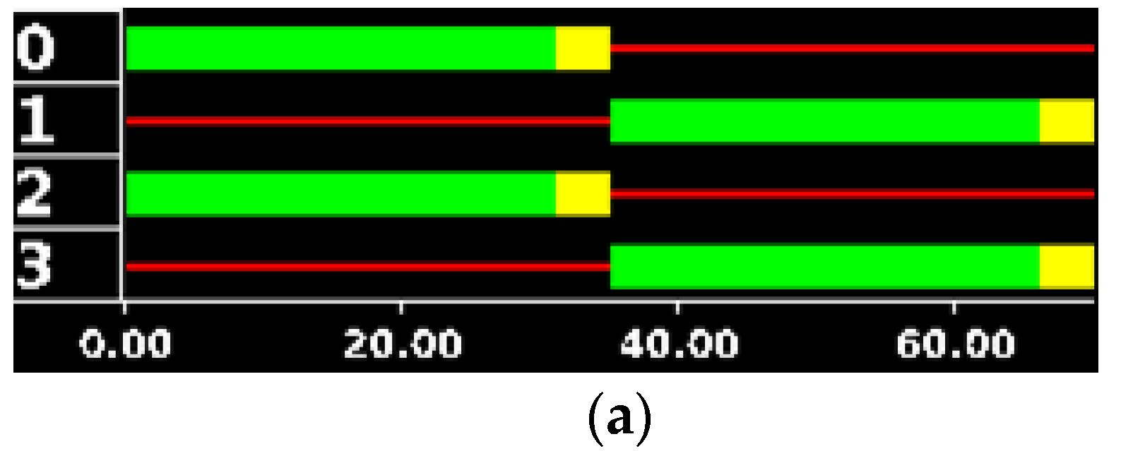
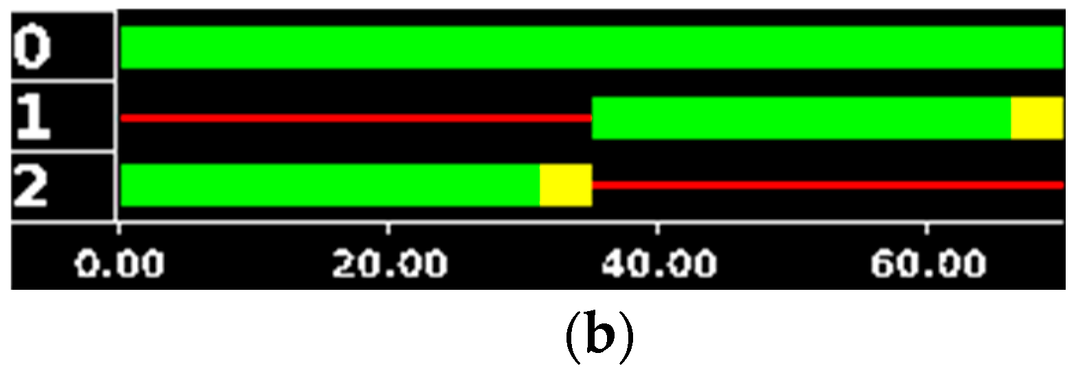
In this scenario, TLCs work with a fixed timing (), because there is no control system running. This initial timing () is shown in Figure 5. The simulation ran 2 h (7200 s) with a simulation step size of 1 s.
We used the SUMO simulator [34] for emulating the urban traffic network. This is a microscopic traffic simulator which enables interaction with an external application through an interface (TraCI: Traffic Control Interface). This simulator feeds traffic information from the traffic detectors, taking raw-pollution data of vehicles and traffic-light actions. TraCI4Matlab [35] is a library of functions for interaction with SUMO from the Matlab command line. It was used for linking SUMO simulator to Matlab models.
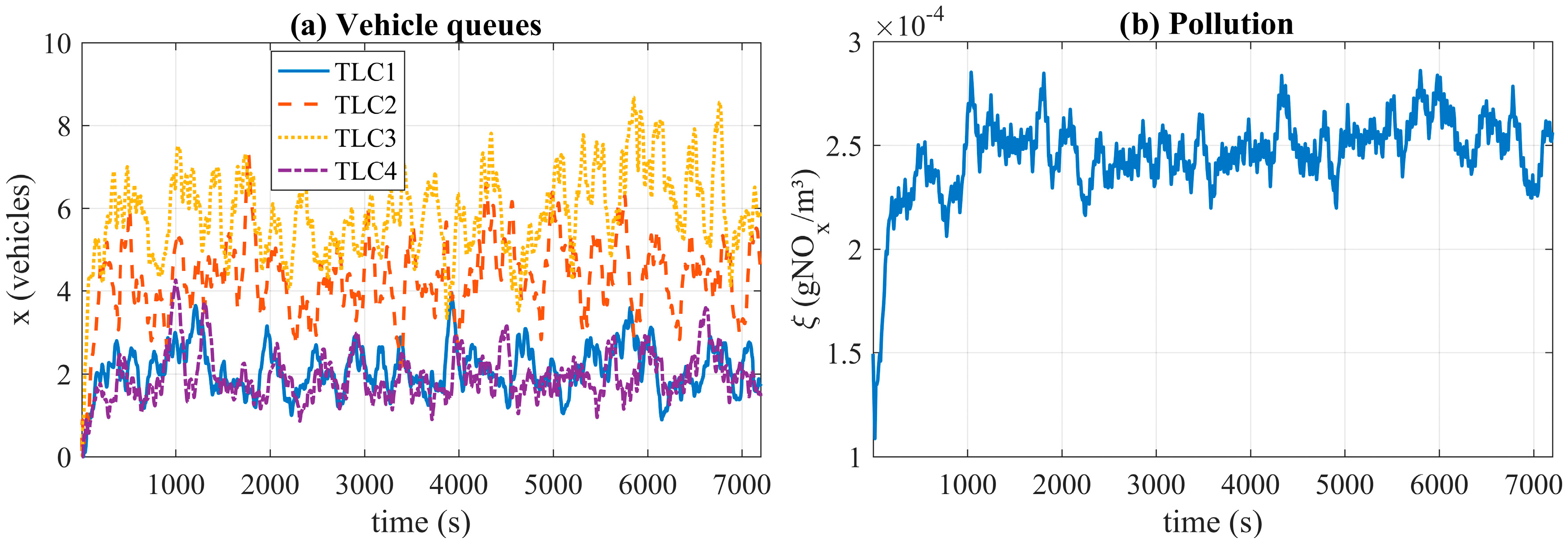
Figure 6a shows the traffic queues obtained at all junctions. The plotted data corresponds to the average vehicle queues at every approach to each junction in a time window of 20 s. Figure 6b shows the average value of NOx emissions of the whole scenario, also in a time window of 20 s. As can be noted, there are no vehicles in the scenario at the beginning of the simulation. Nonetheless, after 100 s from the start of the simulation, the vehicle numbers stabilize.
3.4. Consensus-Based Control Applied to the Test Scenario
In this subsection, the simulation of the cooperative control system in the test scenario is described. The scenario is composed of four interconnected TLCs. The system components and the interaction between them are represented in Figure 7.
The structure of DEVS model for carrying out the study is depicted in Figure 8. MatlabDEVS Toolbox [36] is used for the implementation of the DEVS models and the DEVS simulation. This toolbox has the necessary functions and scripts related with PDEVS formalism, making use of object-oriented language. This toolbox also permits us to run the PDEVS simulator and hybrid simulations by using continuous variables within atomic models.
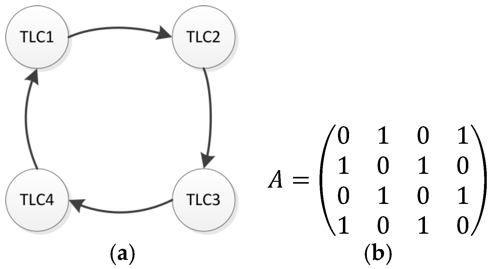
Figure 9 describes the network topology and the associated adjacency matrix. The adjacency matrix represents the connections of the nodes with their neighbors. The communication topology is defined by a directed cycle graph composed of four nodes for this specific test scenario. This communication topology is a key issue for emulating the system behavior. We can extract the adjacency matrix from this representation. If a communication link exists the corresponding value is , otherwise .
For testing the whole system, the scenario was run during 7200 s (2 h) and the control system for TLCs starts at second 100. The following parameters of the models were defined for the simulation of the control system:
- The pollutant considered in this work was NOx. The NOx produced by vehicles was taken from the HBEFA [37], assuming the vehicles were passenger cars built between 2005 and 2015 (0.35 gNOx/veh/km).
- The DEVS model of “Other pollution sources” produces pollution information every 5 s from statistical data of a common urban area, without taking into account the traffic contribution to the pollution. It generates random numbers from the normal distribution with mean: μEo = 30.36 µgNOx/m3 and standard deviation σEo = 10.48 µgNOx/m3.
- The DEVS model “Pollution monitoring” filters the input data by using a moving average filter with a window size of 100 s and outputs a value every 10 s.
- The execution period of TLC DEVS model is 1 s. It filters the input traffic data using a moving average filter with a window size of 100 s.
- The value of was set to 0.15 to guarantee consensus stability ().
- At each TLC, a threshold value of variation of 1% was defined for , in order not to send continuous new values to the traffic lights when the variation of is minimal.
- The value of was estimated by applying a linear regression with values obtained via simulation. The adopted value was 12.68 [veh/% T.L. cycle].
Each TLC calculates the new values of traffic queues (based on vehicles detector sensors placed at each intersection), the consensus variable and the control signal . After that, the cycle length of each traffic light is calculated and updated as , where represents its initial value. Finally, the new value of is sent to the corresponding TLC, in order to modify the cycle length.
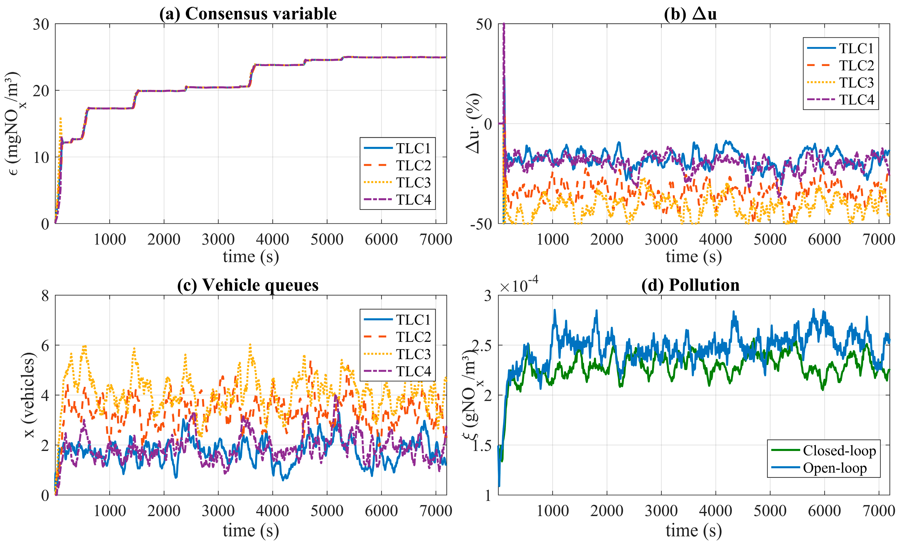
Once the cooperative control is activated at second 100, each TLC begins to exchange information with the neighbors and calculates the control input . Figure 10 shows the simulation results of the interconnected systems. Figure 10a shows the evolution of the consensus variable of each TLC when the control is activated. The consensus variable achieves the same values after 40 s of execution time. Figure 10c shows the amount of vehicles in each intersection () while Figure 10d reflects the total pollution level () in both cases open-loop and closed-loop control. The results depicted in this figure show a reduction in the total pollution level in comparison to the study presented in Section 3.3 without a control mechanism (i.e., open loop).
4. Results and Discussion
The behaviour of the system is highly dependent of traffic conditions, therefore 50 runs for simulating the scenario of both open loop (TLCs work with a fixed timing or ) and closed-loop were performed to carry the comparison. In every new simulation random vehicle routes were generated.
In order to assess the performance of the control system, two key performance indicators (KPIs) were defined, i.e., the mean absolute value of vehicle queues at all intersections and the global pollution during the simulation time (2 h). Both are selected because they serve to evaluate the actual behaviour of the consensus-based control system. The KPIs values are shown in Table 4.
In the case of vehicle queues, the average value for all simulations was 13.48 for open-loop and 12.04 for closed-loop, representing an improvement of 10.70%. Table 4 shows smaller KPIs for closed-loop strategy than open-loop ones. It also demonstrates that vehicle queues are therefore decreased by applying the consensus-based cooperative control system for the urban traffic network. Accordingly, the effect of balancing consensus variables in every TLC produces a global reduction of vehicle queues. As shown in Figure 10b,c, the control system implements a greater decrease in the timing of intersections with larger numbers of vehicles. This makes the number of vehicles at these intersections smaller compared to the case of the open-loop system.
Regarding the key performance indicator related to global pollution, there is a small reduction when the control system is activated. In the case of the mean value of this KPI, the difference between the close-loop and open-loop performance is not as significant as in the case of the KPI related to vehicle queues at all intersections. However, despite the presence of traffic pollution and disturbances in the pollution produced by other sources, we consider that the performance of control system is appropriate since a positive effect is achieved because global pollution is slightly reduced.
5. Conclusions
In this work a cooperative control approach for a smart city environment based on pollution sensing and traffic information is presented. By applying a System-of-Systems engineering design paradigm, a traffic control subsystem uses information from the city pollution sensing system for adjusting the cycle length of the traffic lights. Furthermore, a consensus-based control method was developed to address specific problems related with traffic congestion and air pollution. Discrete event system specification was used to represent and simulate the whole system. This modelling paradigm serves to deal with interoperability of heterogeneous systems.
The proposed method is evaluated in a defined scenario. The study demonstrates that the proposed method is a powerful strategy to deal simultaneously with different sensing systems and for integrating information from pollution levels and traffic flows in urban traffic networks. The results are promising because the number of vehicles in queue decreased, while consensus state variable at each intersection tended towards a common value, demonstrating the validity of the proposed solution. Further research will be conducted to test the solution in larger and more complex scenario and to extend the simulation results to real-time platforms.
Acknowledgments
Authors wish to thank the support given by the project IoSENSE: Flexible FE/BE Sensor Pilot Line for the Internet of Everything, funded by the Electronic Component Systems for European Leadership Joint (ECSEL) Undertaking under grant agreement No 692480.This work has been also supported by MINECO (Spain) through the project RTC-2015-3942-4 TCAP: Auto. Moreover, Raúl M. del Toro acknowledges the financial support received from MINECO through grant “Juan de la Cierva-incorporación”, code IJCI-2014-20169.
Author Contributions
Rodolfo Haber contributed to the review of the state of the art and control system design. Antonio Artuñedo was in charge of modeling and simulation tasks and analyzed the data. Raúl M. del Toro and Antonio Artuñedo designed the scenario, the control system and wrote the paper.
Conflicts of Interest
The authors declare no conflict of interest.
References
- Harrison, C.; Donnelly, I.A. A theory of smart cities. In Proceedings of the 55th Annual Meeting of the ISSS-2011, Hull, UK, 17–22 July 2011. [Google Scholar]
- Naphade, M.; Banavar, G.; Harrison, C.; Paraszczak, J.; Morris, R. Smarter Cities and Their Innovation Challenges. Computer 2011, 44, 32–39. [Google Scholar] [CrossRef]
- Gurgen, L.; Gunalp, O.; Benazzouz, Y.; Gallissot, M. Self-aware cyber-physical systems and applications in smart buildings and cities. Presented at 2013 Design, Automation & Test in Europe Conference & Exhibition (DATE), Grenoble, France, 18–22 March 2013; pp. 1149–1154. [Google Scholar]
- Sánchez Boza, A.; Guerra, R.H.; Gajate, A. Artificial cognitive control system based on the shared circuits model of sociocognitive capacities. A first approach. Eng. Appl. Artif. Intell. 2011, 24, 209–219. [Google Scholar] [CrossRef]
- Precup, R.-E.; Angelov, P.; Costa, B.S.J.; Sayed-Mouchaweh, M. An overview on fault diagnosis and nature-inspired optimal control of industrial process applications. Comput. Ind. 2015, 74, 75–94. [Google Scholar] [CrossRef]
- Boardman, J.; Sauser, B. System of Systems—The meaning of of. Presented at 2006 IEEE/SMC International Conference on System of Systems Engineering, Los Angeles, CA, USA, 24–26 April 2006; p. 6. [Google Scholar]
- Adler, J.L.; Blue, V.J. Toward the design of intelligent traveler information systems. Transp. Res. Part C Emerg. Technol. 1998, 6, 157–172. [Google Scholar] [CrossRef]
- Nanayakkara, T.; Sahin, F.; Jamshidi, M. Intelligent Control. Systems with an Introduction to System of Systems Engineering; CRC Press: Boca Raton, FL, USA, 2010. [Google Scholar]
- Ren, W.; Beard, R. Distributed Consensus in Multi-Vehicle Cooperative Control: Theory and Applications; Springer: London, UK, 2007. [Google Scholar]
- Joordens, M.A.; Jamshidi, M. Consensus Control for a System of Underwater Swarm Robots. IEEE. Syst. J. 2010, 4, 65–73. [Google Scholar] [CrossRef]
- Fax, J.A.; Murray, R.M. Information flow and cooperative control of vehicle formations. IEEE Trans. Autom Control 2004, 49, 1465–1476. [Google Scholar] [CrossRef]
- Qu, Z.; Jing, W.; Hull, R.A. Cooperative Control of Dynamical Systems with Application to Autonomous Vehicles. IEEE Trans. Autom Control 2008, 53, 894–911. [Google Scholar] [CrossRef]
- Kim, B.Y.; Ahn, H.S. Distributed Coordination and Control for a Freeway Traffic Network Using Consensus Algorithms. IEEE Syst. J. 2016, 10, 162–168. [Google Scholar] [CrossRef]
- Wang, Z.; Sui, C. Distributed traffic network control system. Presented at 2013 IEEE International Conference on Signal Processing, Communication and Computing (ICSPCC), Kunming, China, 5–8 August 2013; pp. 1–4. [Google Scholar]
- He, Z.H.; Chen, Y.Z.; Shi, J.J.; Wu, X.; Guan, J.Z. Consensus based Approach to the Signal Control of Urban Traffic Networks. Procedia Soc. Behav. Sci. 2013, 96, 2511–2522. [Google Scholar]
- Safarinejadian, B.; Estahbanati, M.E. Consensus Filter-Based Distributed Variational Bayesian Algorithm for Flow and Speed Density Prediction With Distributed Traffic Sensors. IEEE Syst. J. 2015, PP, 1–10. [Google Scholar] [CrossRef]
- Jeličić, V.; Tolic, D.; Bilas, V. Consensus-based decentralized resource sharing between co-located Wireless Sensor Networks. Presented at 2014 IEEE Ninth International Conference on Intelligent Sensors Sensor Networks and Information Processing (ISSNIP), Singapore, 21–24 April 2014; pp. 1–6. [Google Scholar]
- Castro, G.; Martini, J.; Hirakawa, A. Multilayer distributed model predictive control of urban traffic. WIT Trans. Ecol. Environ. 2013, 179, 967–976. [Google Scholar]
- Wuthishuwong, C.; Traechtler, A. Consensus Coordination in the Network of Autonomous Intersection Management. Presented at Conference on Informatics in Control, Automation and Robotics (ICINCO), 2014 11th International, Vienna, Australia, 1–3 September 2014. [Google Scholar]
- Zeigler, B.P.; Sarjoughian, H.S. Guide to Modeling and Simulation of Systems of Systems; Springer: London, UK, 2013. [Google Scholar]
- Zanella, A.; Bui, N.; Castellani, A.; Vangelista, L.; Zorzi, M. Internet of Things for Smart Cities. IEEE Internet Things J. 2014, 1, 22–32. [Google Scholar] [CrossRef]
- Srbinovski, B.; Magno, M.; Edwards-Murphy, F.; Pakrashi, V.; Popovici, E. An Energy Aware Adaptive Sampling Algorithm for Energy Harvesting WSN with Energy Hungry Sensors. Sensors 2016, 16, 448. [Google Scholar] [CrossRef] [PubMed]
- Kumar, P.; Morawska, L.; Martani, C.; Biskos, G.; Neophytou, M.; di Sabatino, S.; Bell, M.; Norford, L.; Britter, R. The rise of low-cost sensing for managing air pollution in cities. Environ. Int. 2015, 75, 199–205. [Google Scholar] [CrossRef] [PubMed]
- Penza, M.; Suriano, D.; Villani, M.G.; Spinelle, L.; Gerboles, M. Towards air quality indices in smart cities by calibrated low-cost sensors applied to networks. Presented at IEEE SENSORS 2014, Valencia, Spain, 2–5 November 2014; pp. 2012–2017. [Google Scholar]
- Nellore, K.; Hancke, G. A Survey on Urban Traffic Management System Using Wireless Sensor Networks. Sensors 2016, 16, 157. [Google Scholar] [CrossRef] [PubMed]
- Imawan, A.; Indikawati, F.I.; Kwon, J.; Rao, P. Querying and extracting timeline information from road traffic sensor data. Sensors 2016, 16, 1340. [Google Scholar] [CrossRef] [PubMed]
- Klein, L.A.; Mills, M.K.; Gibson, D.R. Traffic Detector Handbook; U.S. Department of Transportation: Washington, DC, USA, 2006; Volume II.
- Ando, B.; Baglio, S.; Graziani, S.; Pecora, E.; Pitrone, N. A predictive model for urban air pollution evaluation. Procceding of the IMTC/97 Instrumentation and Measurement Technology Conference, Ottawa, ON, Canada, 19–21 May 1997. [Google Scholar]
- Hamilton, A.; Waterson, B.; Cherrett, T.; Robinson, A.; Snell, I. The evolution of urban traffic control: Changing policy and technology. Transp. Plan. Technol. 2013, 36, 24–43. [Google Scholar] [CrossRef]
- Wainer, G.A.; Mosterman, P.J. Discrete-Event Modeling and Simulation: Theory and Applications; CRC Press: Boca Raton, FL, USA, 2010. [Google Scholar]
- Belalcazar, L.C.; Fuhrer, O.; Ho, M.D.; Zarate, E.; Clappier, A. Estimation of road traffic emission factors from a long term tracer study. Atmos. Environ. 2009, 43, 5830–5837. [Google Scholar] [CrossRef]
- Olfati-Saber, R.; Fax, J.A.; Murray, R.M. Consensus and Cooperation in Networked Multi-Agent Systems. Proc. IEEE 2007, 95, 215–233. [Google Scholar] [CrossRef]
- Krauß, S. Microscopic Modeling of Traffic Flow: Investigation of Collision Free Vehicle Dynamics. Ph.D. Thesis, Universitat zu Koln, Koln, Germany, 1998. [Google Scholar]
- Krajzewicz, D.; Erdmann, J.; Behrisch, M.; Bieker, L. Recent development and applications of SUMO–simulation of urban mobility. Int. J. Adv. Syst. Meas. 2012, 5, 128–138. [Google Scholar]
- Acosta, A.; Espinosa, J.; Espinosa, J. TraCI4Matlab: Enabling the Integration of the SUMO Road Traffic Simulator and Matlab® Through a Software Re-engineering Process. In Modeling Mobility with Open Data; Behrisch, M., Weber, M., Eds.; Springer International Publishing: Berlin, Germany, 2015; pp. 155–170. [Google Scholar]
- Pawletta, T.; Deatcu, C.; Pawletta, S.; Hagendorf, O.; Colquhoun, G. DEVS-based modeling and simulation in scientific and technical computing environments. Simul. Ser. 2006, 38, 151. [Google Scholar]
- Rexeis, M.; Hausberger, S.; Kühlwein, J.; Luz, R. Update of Emission Factors for Euro 5 and Euro 6 Vehicles for the HBEFA Version 3.2; TUG Report I-31/2013/Rex EM-I 2011/20/679 TU Graz; Graz University of Technology: Graz, Austria, 2014; Available online: http://www.hbefa.net/ (accessed on 19 May 2015).
Figure 1.
The schematic concept of a vehicle emission control system.

Figure 2.
Diagram of the general scenario.

Figure 3.
Structure of DEVS models.

Figure 4.
Simulated road network.

Figure 5.
Initial timing of J3 (a), initial timing of J1, J2 and J4 (b).


Figure 6.
Vehicle queues (a) and pollution behavior (b) in an open-loop simulation.

Figure 7.
TLCs interaction scheme.

Figure 8.
Schematic DEVS models for the test scenario.

Figure 9.
Network communication topology (a) and associated adjacency matrix (b).

Figure 10.
Close-loop simulation results: (a) Consensus variable (); (b) Control input (); (c) Vehicle queues (); (d) Pollution level () (closed-loop and open-loop).
Figure 10.
Close-loop simulation results: (a) Consensus variable (); (b) Control input (); (c) Vehicle queues (); (d) Pollution level () (closed-loop and open-loop).


Table 1.
Description of data flows.
| Variable | Description |
|---|---|
| Ev | Vehicle emissions monitoring |
| Eo | Other emissions |
| Area-wide air-quality information. Includes current pollution-status details for a given geographic area. | |
| Consensus variable that represents the TLC dynamics (see Section 3.2.1) | |
| Processed traffic-detector data which allows derivation of traffic-flow variables (density, occupancy, flow measures, etc.). It can be represented as a vector that refers to the signal of each sensor. | |
| Data flow contains the system configuration data for a traffic signal controller. It includes the parameters required to reconfigure its operations. |
Table 2.
Components of the control method
| Component | Expression | Description |
|---|---|---|
| 1 | Feed-forward action related to local pollution data. | |
| 2 | Feed-forward action related to local traffic data. | |
| 3 | Consensus-based control signal that makes use of information from the neighbor of each network node. |
Table 3.
Vehicle and car-following model parameters.
| Variable | Value |
|---|---|
| Length (m) | 5.00 |
| Minimum gap (m) | 2.50 |
| Maximum speed (m/s) | 55.56 |
| Maximum acceleration (m/s2) | 2.60 |
| Maximum deceleration (m/s2) | 4.50 |
| Imperfection | 0.50 |
| Reaction time (s) | 1.00 |
| Person capacity | 4 |
Table 4.
KPIs for the evaluation of the control system.
| KPI | Open-Loop | Closed-Loop | Differences Relative to Open-Loop | |
|---|---|---|---|---|
| Vehicle queues 1. | μ | 13.4815 | 12.0382 | 10.70% |
| max | 15.0661 | 13.6345 | 9.50% | |
| Global pollution 2. | μ | 2.3879×10⁻⁴ | 2.3791×10⁻⁴ | 0.37% |
| min | 2.2732×10⁻⁴ | 2.1910×10⁻⁴ | 3.62% | |
© 2017 by the authors. Licensee MDPI, Basel, Switzerland. This article is an open access article distributed under the terms and conditions of the Creative Commons Attribution (CC BY) license (http://creativecommons.org/licenses/by/4.0/).
Share and Cite
MDPI and ACS Style
Artuñedo, A.; Del Toro, R.M.; Haber, R.E. Consensus-Based Cooperative Control Based on Pollution Sensing and Traffic Information for Urban Traffic Networks. Sensors 2017, 17, 953. https://doi.org/10.3390/s17050953
AMA Style
Artuñedo A, Del Toro RM, Haber RE. Consensus-Based Cooperative Control Based on Pollution Sensing and Traffic Information for Urban Traffic Networks. Sensors. 2017; 17(5):953. https://doi.org/10.3390/s17050953
Chicago/Turabian StyleArtuñedo, Antonio, Raúl M. Del Toro, and Rodolfo E. Haber. 2017. "Consensus-Based Cooperative Control Based on Pollution Sensing and Traffic Information for Urban Traffic Networks" Sensors 17, no. 5: 953. https://doi.org/10.3390/s17050953
Note that from the first issue of 2016, this journal uses article numbers instead of page numbers. See further details here.