
A Cost-Effective Geodetic Strainmeter Based on Dual Coaxial Cable Bragg Gratings

Abstract
:1. Introduction
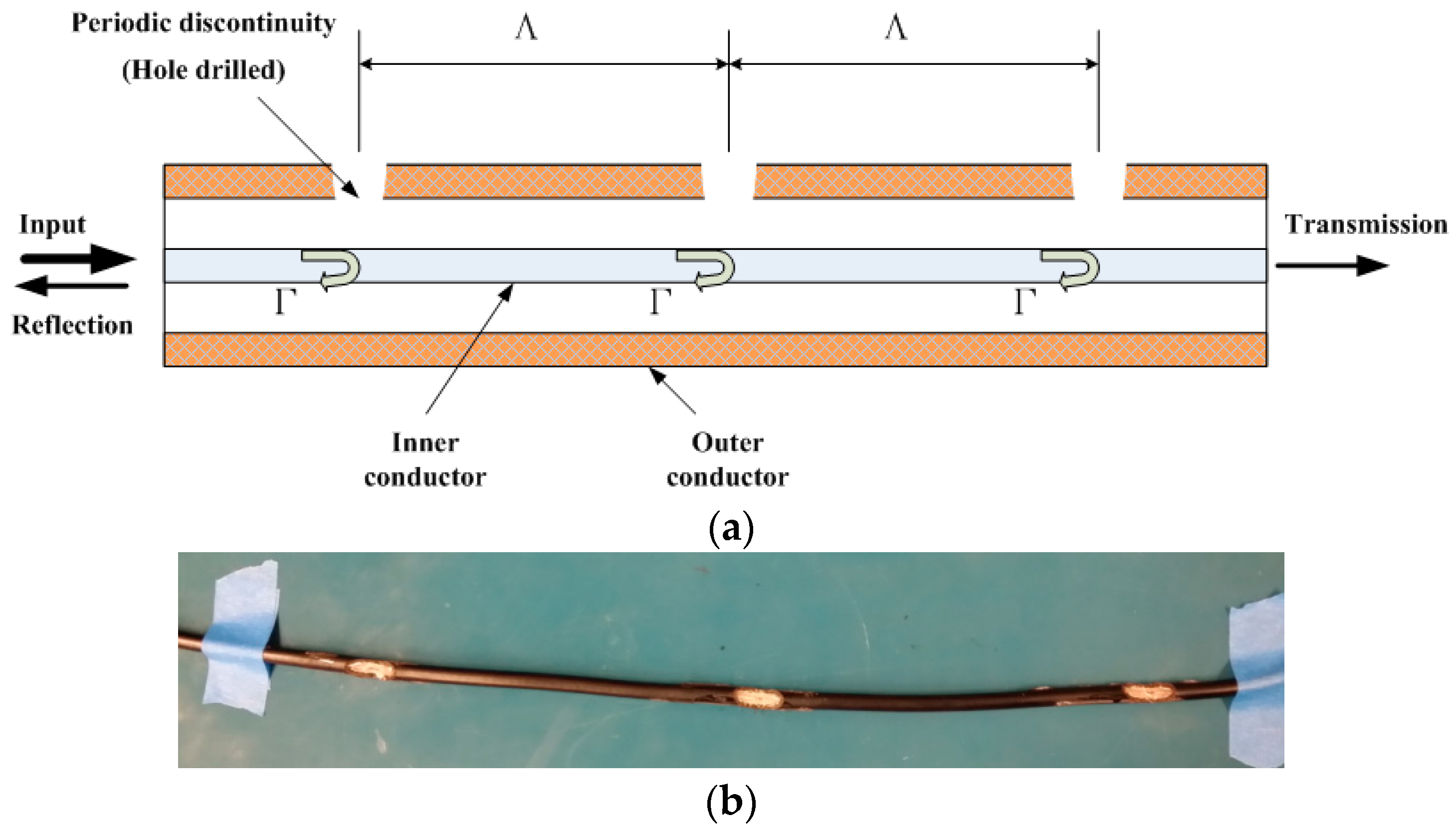
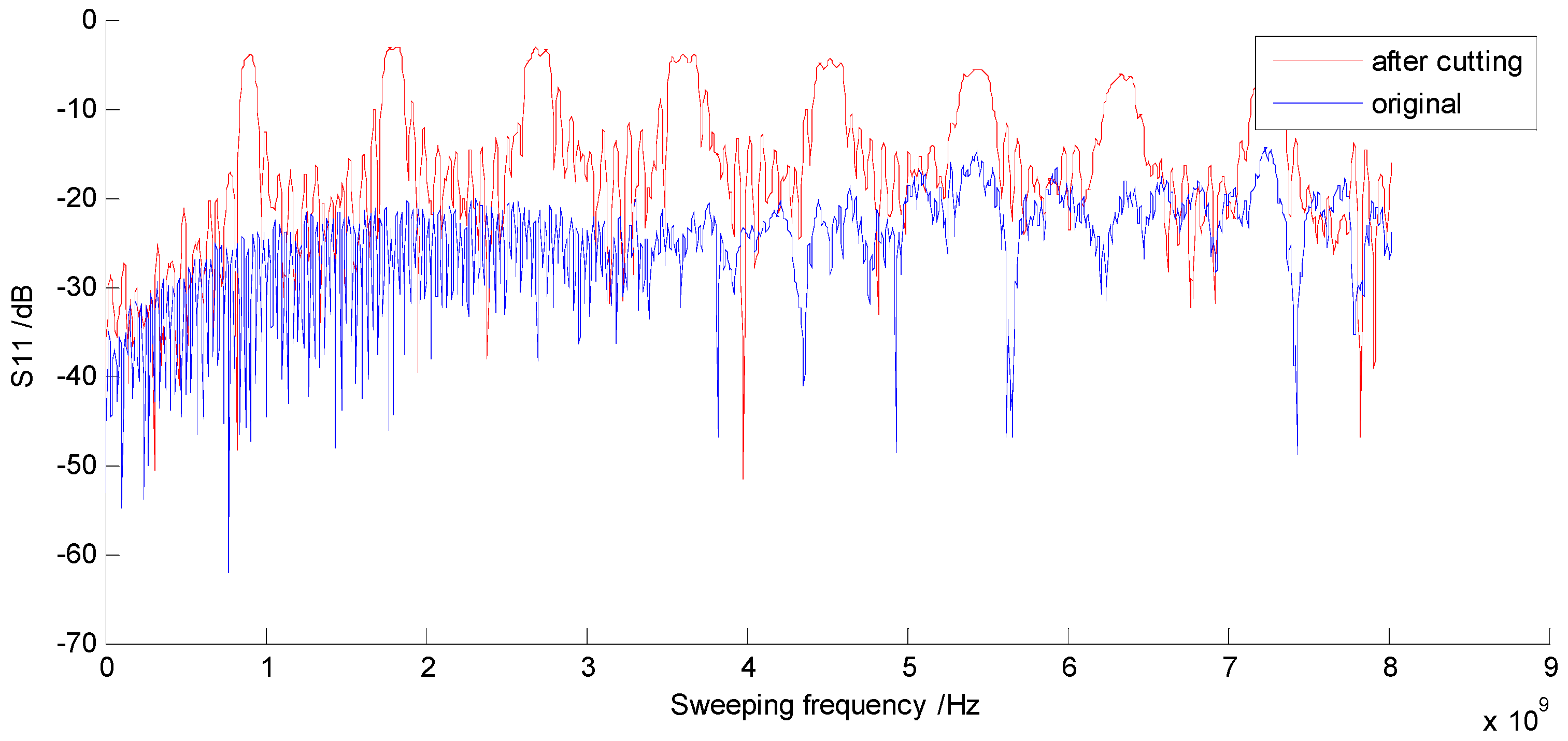
2. Working Principle of CCBG
3. Geodetic Strainmeter Design
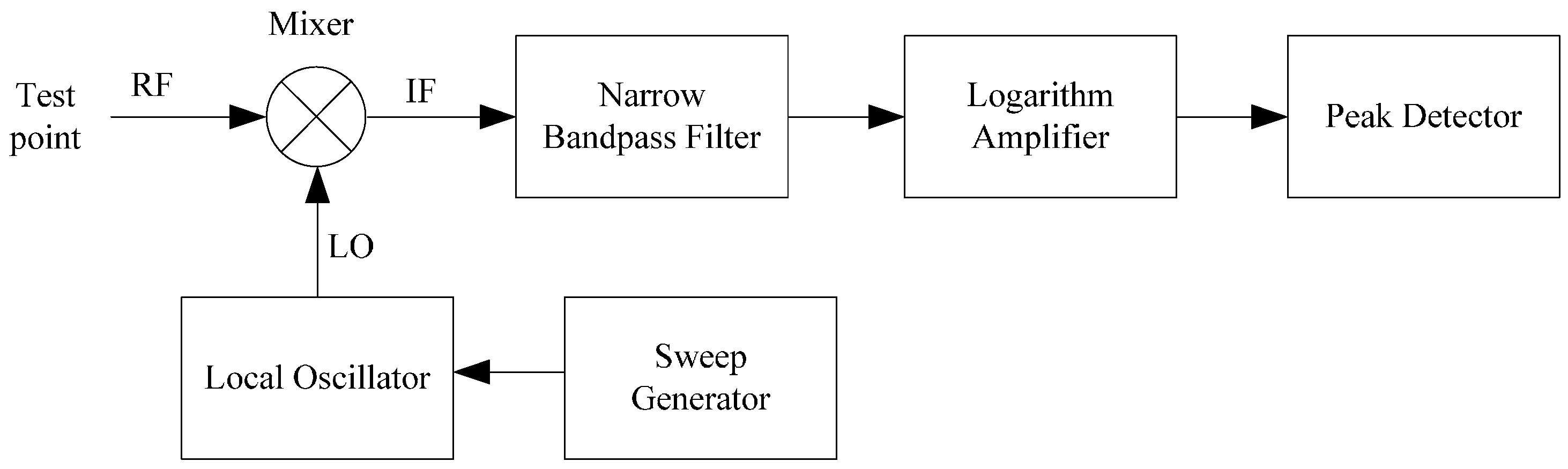
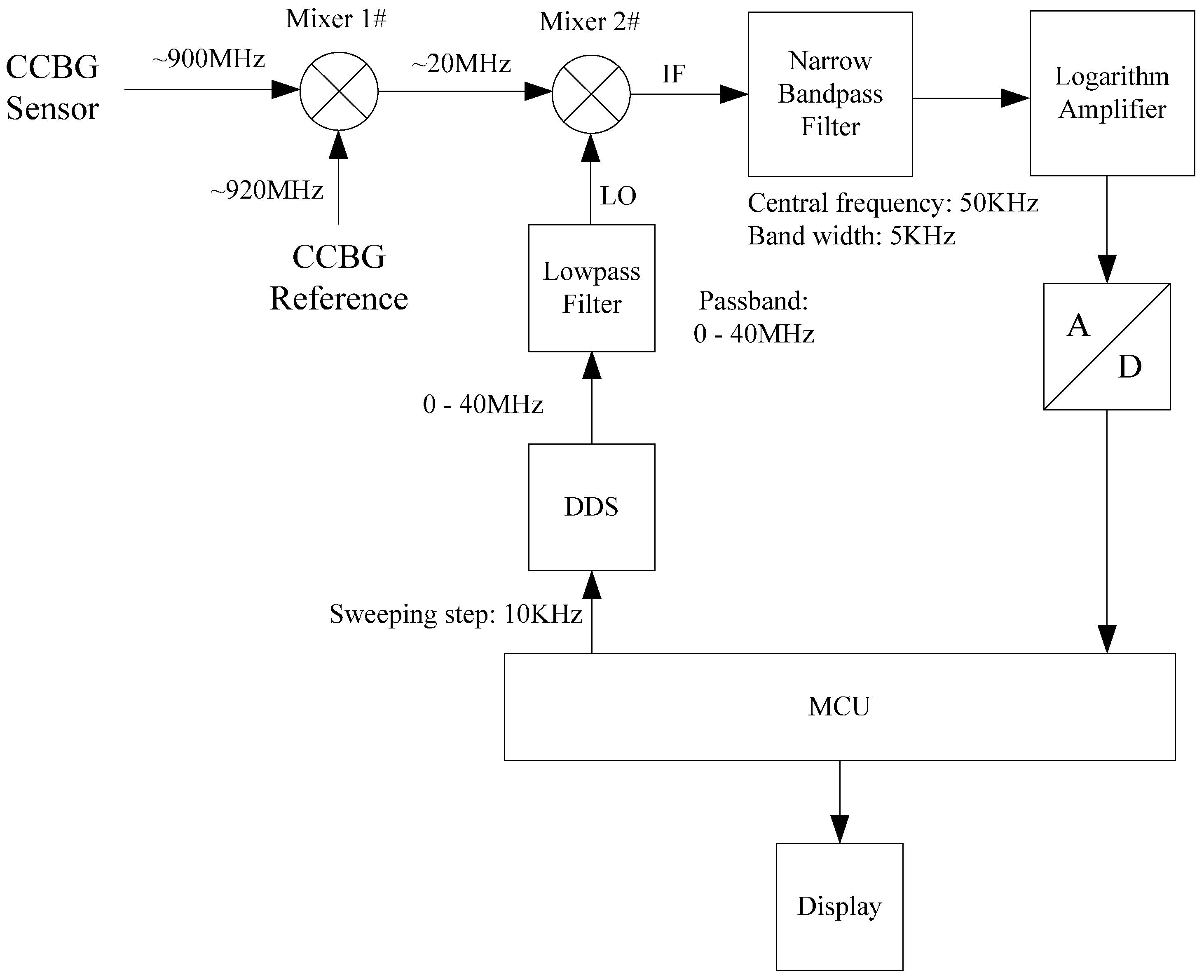
3.1. Hardware Design
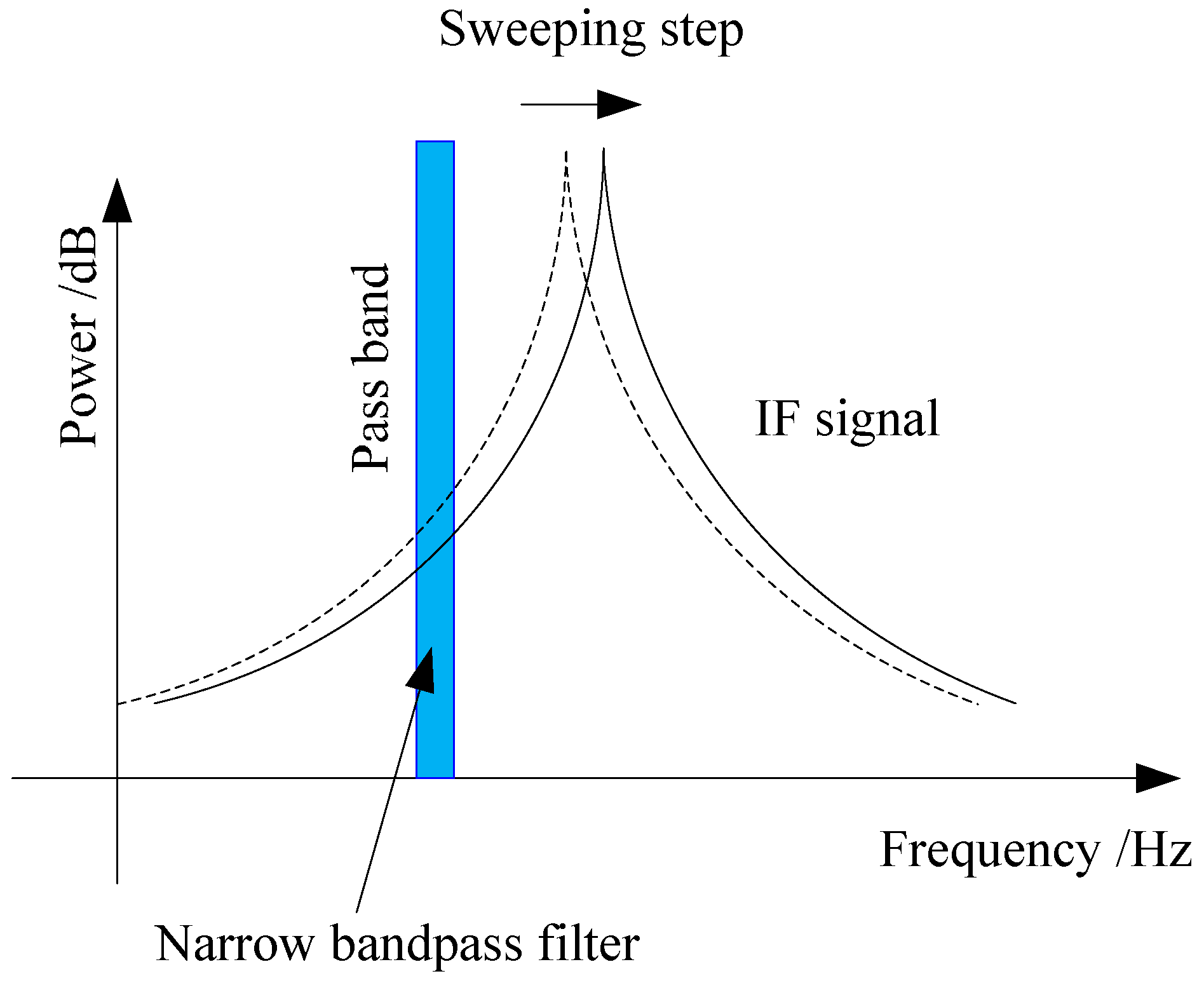
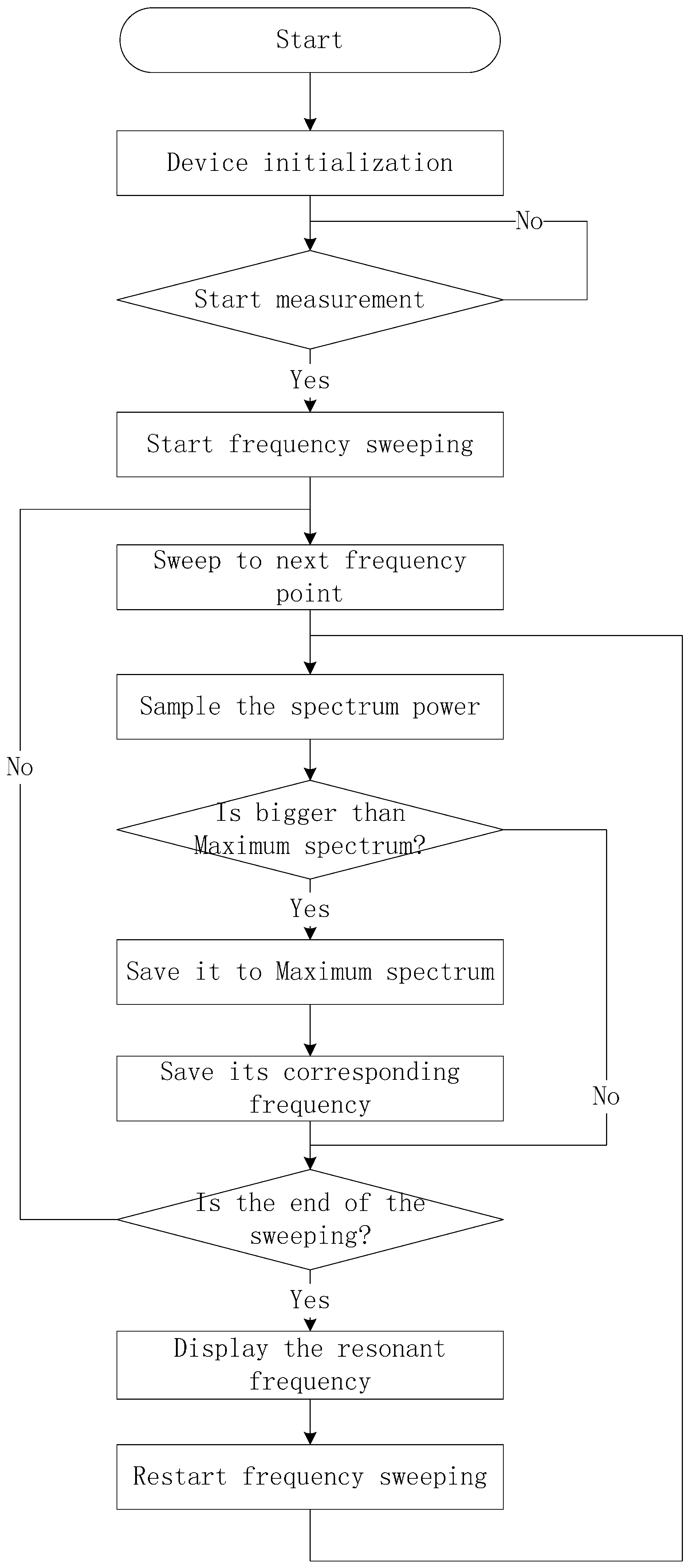
3.2. Software Design
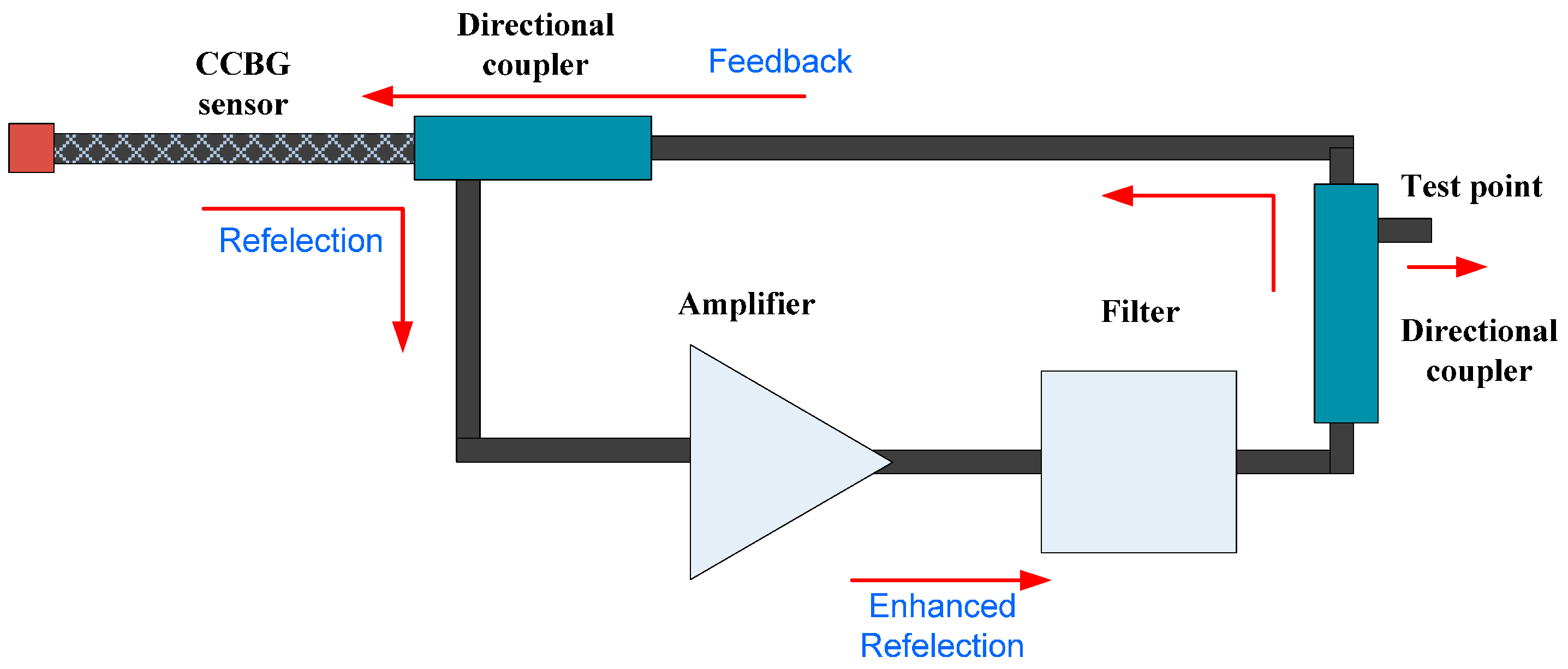
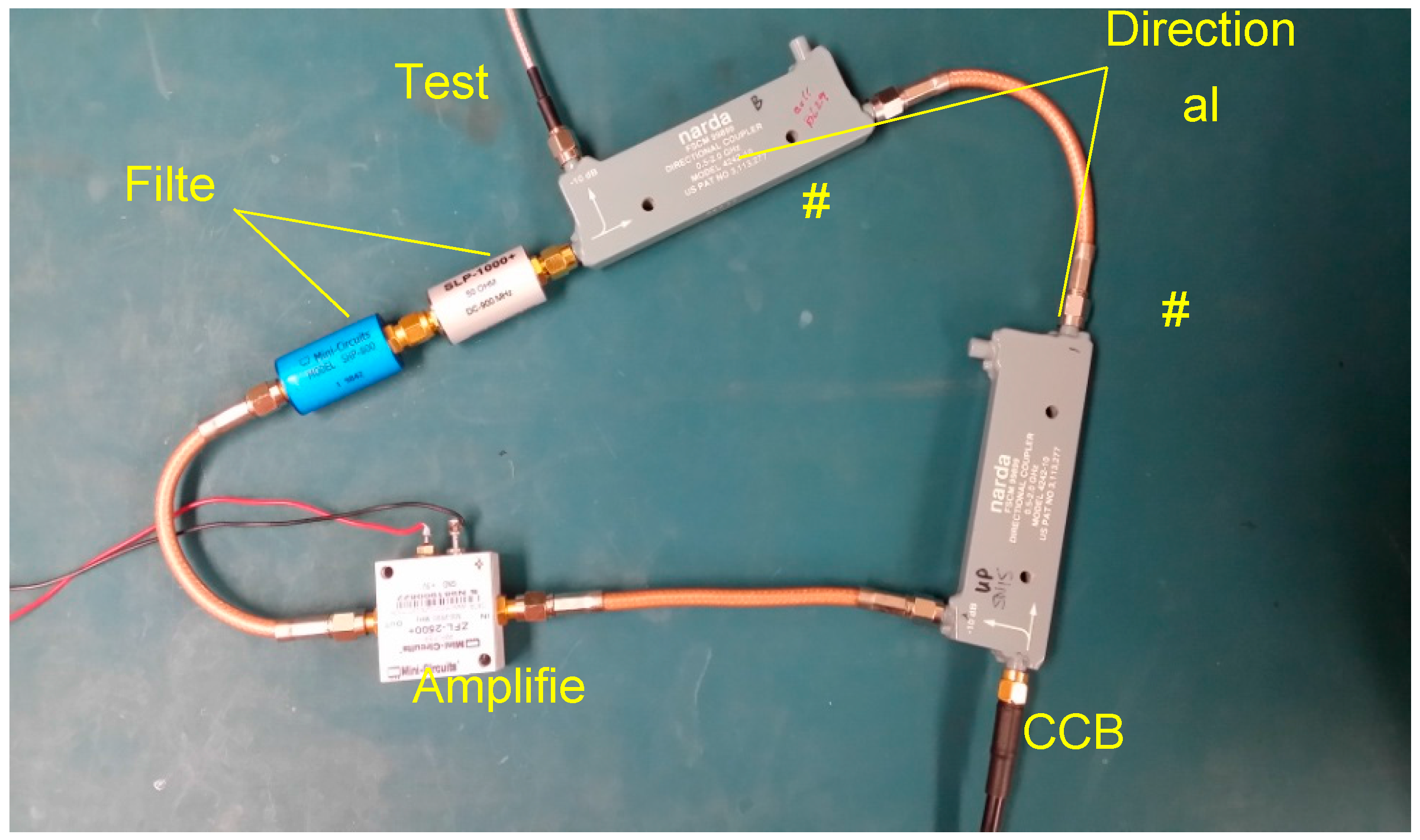
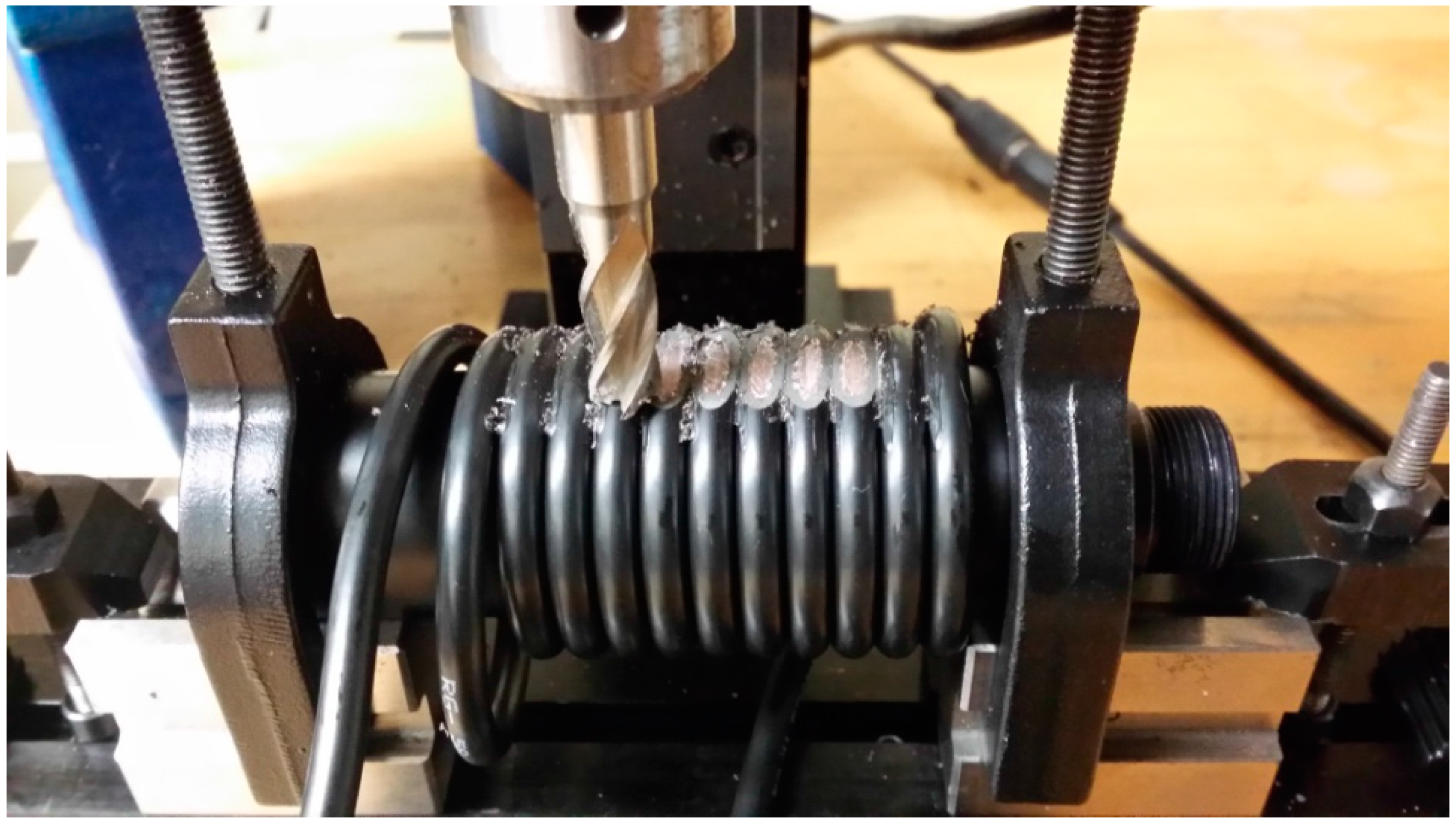
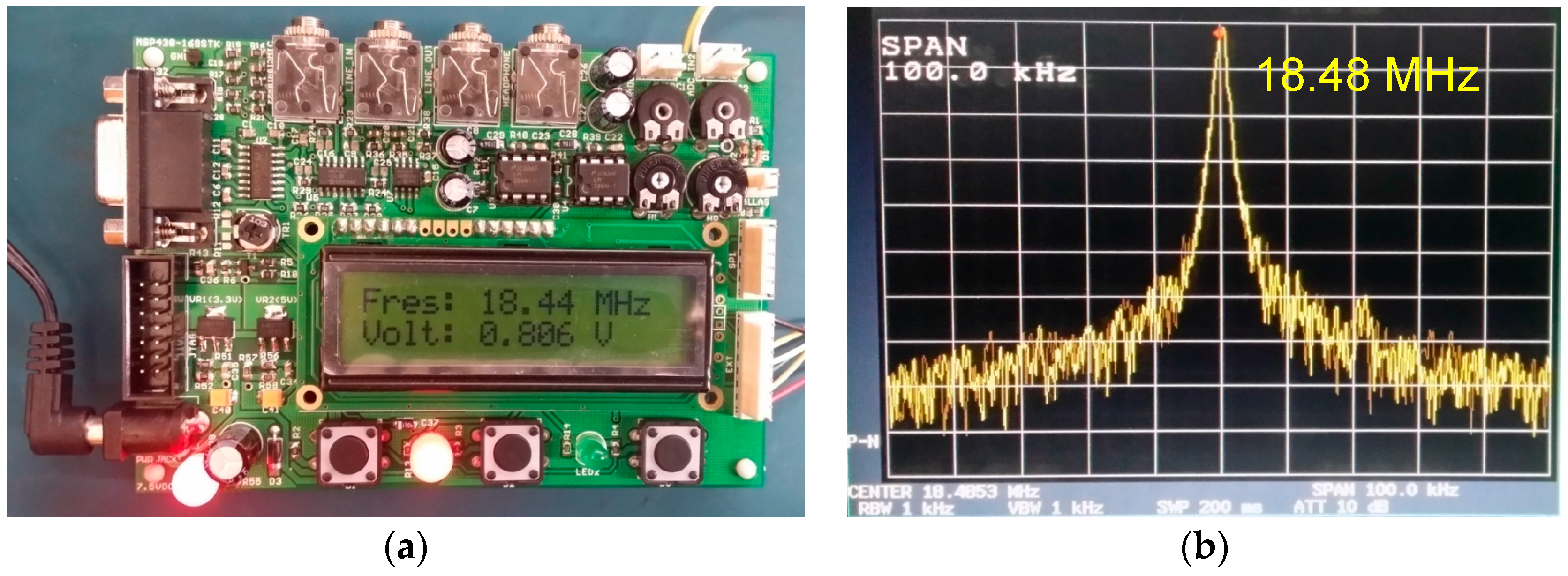
4. Demo System
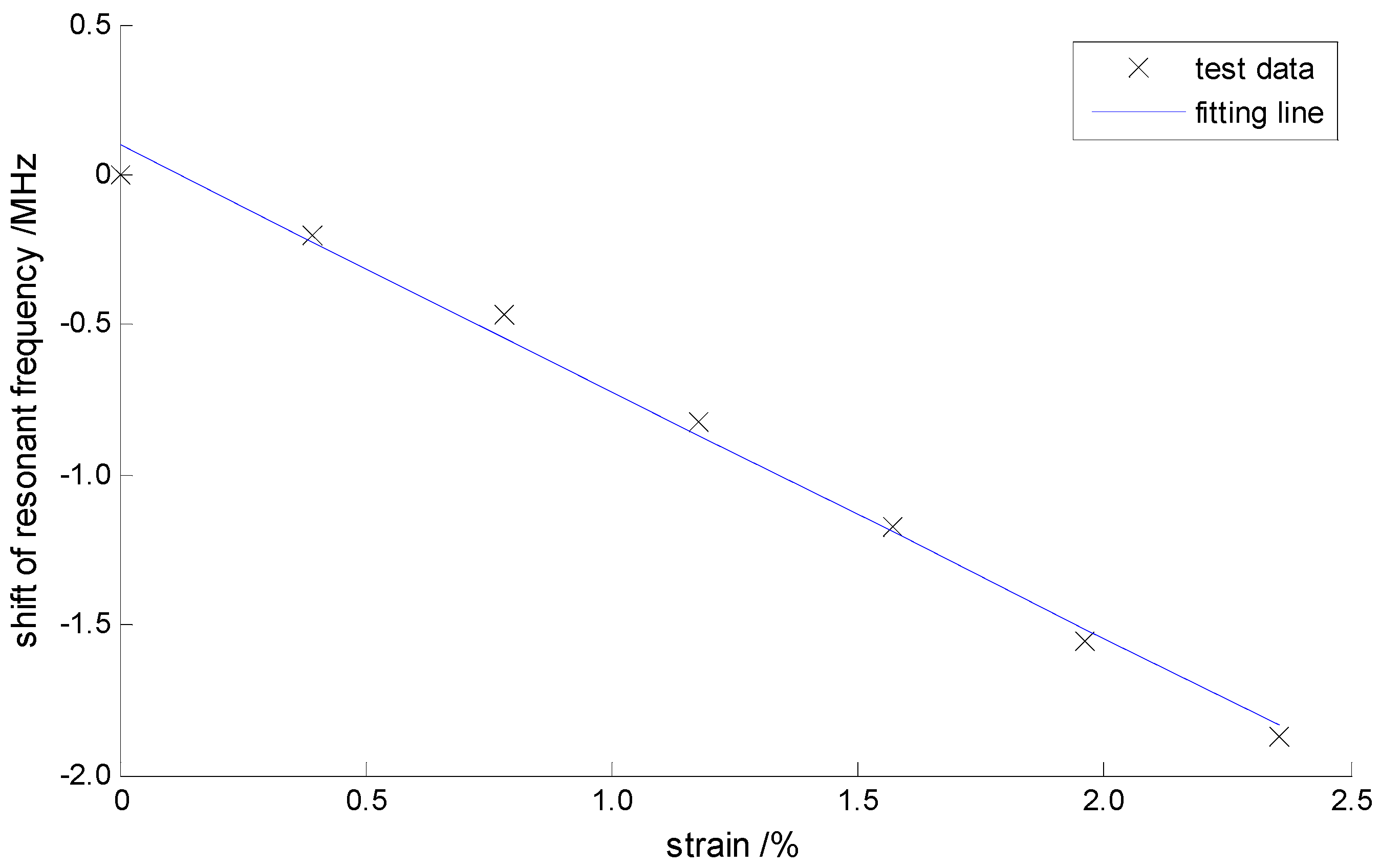
5. Results
6. Conclusions
Acknowledgments
Author Contributions
Conflicts of Interest
References
- Simons, M.; Minson, S.E.; Sladen, A.; Sladen, A.; Ortega, F.; Jiang, J.; Owen, S.E.; Meng, L.; Wei, S.; Chu, R.; et al. The 2011 magnitude 9.0 Tohoku-Oki earthquake: Mosaicking the megathrust from seconds to centuries. Science 2011, 332, 1421–1425. [Google Scholar] [CrossRef] [PubMed]
- Sato, M.T.; Ishikawa, T.; Ujihara, N.; Yoshida1, S.; Fujita, M.; Mochizuki, M.; Asada, A. Displacement above the hypocenter of the 2011 Tohoku-Oki earthquake. Science 2011, 332, 1395. [Google Scholar] [CrossRef] [PubMed]
- EarthScope. Available online: http://www.earthscope.org/ (accessed on 20 June 2014).
- Crustal Movement Observation Network of China. Available online: http://www.neiscn.org/ (accessed on 2 July 2014). (In Chinese).
- Yin, H.; Zhang, P.; Gan, W.; Wang, M.; Liao, H.; Li, X.; Li, X.; Xiao, G. Near-field surface movement during the Wenchuan Ms8.0 earthquake measured by high-rate GPS. Chin. Sci. Bull. 2010, 55, 2621–2626. [Google Scholar] [CrossRef]
- Araya, A. Iodine-stabilized 633 nm He-Ne laser for long-baseline interferometers. Jpn. J. Appl. Phys. 1997, 36, 3515–3516. [Google Scholar] [CrossRef]
- Nissen, E.; Maruyama, T.; Arrowsmith, J.R.; Elliott, J.R.; Krishnan, A.K.; Oskin, M.E.; Saripalli, S. Coseismic fault zone deformation revealed with differential lidar: Examples from Japanese Mw~7 intraplate earthquakes. Earth Planet. Sci. Lett. 2014, 405, 244–256. [Google Scholar] [CrossRef]
- Kersey, A.D.; Davis, M.A.; Patrick, H.J.; LeBlanc, M.; Koo, C.P.; Askins, C.G.; Putnam, M.A.; Friebele, E.J. Fiber grating sensors. J. Lightw. Technol. 1997, 15, 1442–1463. [Google Scholar] [CrossRef]
- Kuang, K.S.C.; Quek, S.T.; Tan, C.Y.; Chew, S.H. Plastic optical fiber sensors for measurement of large strain in geotextile materials. Adv. Mater. Res. 2008, 47–50, 1233–1236. [Google Scholar] [CrossRef]
- Wei, T.; Wu, S.P.; Huang, J.; Fan, J. Coaxial cable Bragg grating. Appl. Phys. Lett. 2011, 99, 113517. [Google Scholar] [CrossRef]
- Wu, S.P.; Wei, T.; Huang, J.; Xiao, H.; Fan, J. Modeling of coaxial cable bragg grating by coupled mode theory. IEEE Sens. J. 2014, 62, 2251–2259. [Google Scholar] [CrossRef]
- Huang, J.; Wei, T.; Lan, X.W.; Fan, J.; Xiao, H. Coaxial cable bragg grating sensors for large strain measurement with high accuracy. Proc. SPIE 2012, 8345. [Google Scholar] [CrossRef]
- Wu, S.P. Modeling of Novel Coaxial Cable Bragg Grating Sensor by Coupled Mode Theory. Ph.D. Thesis, Missouri University of Science and Technology, Rolla, MO, USA, 2011; p. 2214. [Google Scholar]


| Part | Item | Symbol | Value | Comments |
|---|---|---|---|---|
| Demo system | Measuring range | D | ±20,000 με (2%) | respected |
| Resolution | R | 20 με | respected | |
| CCBG sensor | Resonant frequency | fres | 900 MHz | designed |
| Theory sensitivity | A | −0.7 kHz/με | by Equation (3) | |
| Resolution in frequency | Rf | 14.00 kHz | |AR| | |
| Output Range | 900 ± 14 MHz | fres ± |AD| | ||
| CCBG reference | Resonant frequency | fref | 920 MHz | designed |
| Narrow bandpass filter | Central frequency | f0 | 50 kHz | designed |
| Band width | fbw | 5 kHz | <Rf/2 | |
| DDS | Sweeping frequency | fwp | 0 to 40 MHz | >(fref − fres) ± |AD| |
| Sweeping step | fstp | 10 kHz | <Rf | |
| Low pass filter | Passband | 0 to 40 MHz | same as fwp |
| No. | Portable Spectrum Analyzer’s/MHz | R3272’s/MHz | Relative Error/% |
|---|---|---|---|
| 1 | 18.44 | 18.48 | −0.22 |
| 2 | 17.32 | 17.38 | −0.34 |
| 3 | 16.56 | 16.59 | −0.18 |
| 4 | 15.87 | 15.92 | −0.31 |
| No. | Strains/% | Frequency Shifts/MHz | Nonlinear Errors/% |
|---|---|---|---|
| 1 | 0 | 0 | 5.28 |
| 2 | 0.392% | −0.20 | −1.36 |
| 3 | 0.784% | −0.47 | −4.19 |
| 4 | 1.176% | −0.82 | −2.65 |
| 5 | 1.569% | −1.17 | −1.11 |
| 6 | 1.961% | −1.55 | 2.07 |
| 7 | 2.353% | −1.87 | 1.97 |
© 2017 by the authors. Licensee MDPI, Basel, Switzerland. This article is an open access article distributed under the terms and conditions of the Creative Commons Attribution (CC BY) license (http://creativecommons.org/licenses/by/4.0/).
Share and Cite
Fu, J.; Wang, X.; Wei, T.; Wei, M.; Shen, Y. A Cost-Effective Geodetic Strainmeter Based on Dual Coaxial Cable Bragg Gratings. Sensors 2017, 17, 842. https://doi.org/10.3390/s17040842
Fu J, Wang X, Wei T, Wei M, Shen Y. A Cost-Effective Geodetic Strainmeter Based on Dual Coaxial Cable Bragg Gratings. Sensors. 2017; 17(4):842. https://doi.org/10.3390/s17040842
Chicago/Turabian StyleFu, Jihua, Xu Wang, Tao Wei, Meng Wei, and Yang Shen. 2017. "A Cost-Effective Geodetic Strainmeter Based on Dual Coaxial Cable Bragg Gratings" Sensors 17, no. 4: 842. https://doi.org/10.3390/s17040842