Modeling and Density Estimation of an Urban Freeway Network Based on Dynamic Graph Hybrid Automata


Abstract
:1. Introduction
2. Preliminaries
2.1. Dynamic Graph
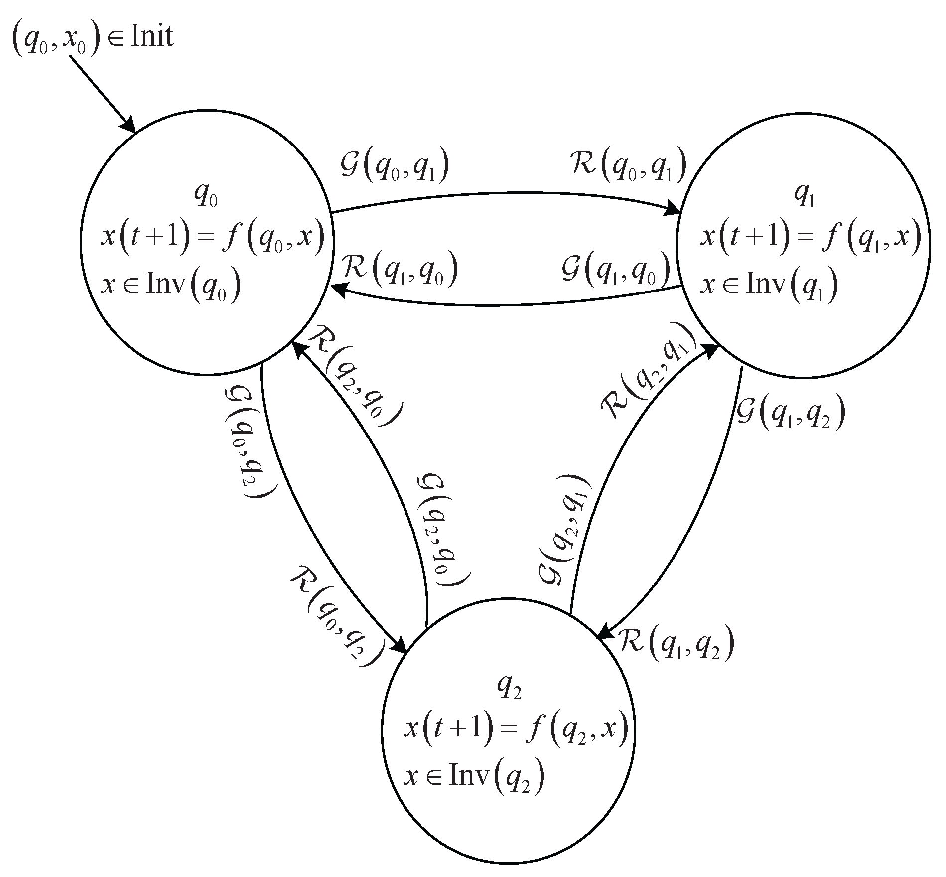
2.2. Hybrid Automaton
- is a state space of hybrid state variables , where Q is a finite set of discrete states q and is a n-dimensional state space of continuous state vector x;
- is a set of initial hybrid states;
- is a set of continuous input variable u;
- is a vector field describing the continuous state dynamics defined by
- is a transition map describing the discrete state dynamics. One can also use a binary relation set to express the discrete state transition;
- defines the domain of continuous state vector under each discrete state. The domain is also called invariant set of continuous state vector;
- defines a guard condition for each discrete state transition;
- is a reset map to assign a new initial state to the continuous state variable after the transition of the discrete state.
- is a set of continuous output variable y;
- is an output map defined as
2.3. Dynamic Graph Hybrid Automata
- (1)
- Fully weighted dynamic digraph. In , is a finite set of N fixed vertices, and is a set of directed edges, and Φ are sets of the automata and the functions that assign the vertex weights and edge weights, respectively, which are described in detail as follows;
- (2)
- Vertex dynamics. The elements in are hybrid automata to describe the dynamics of vertex , whose components are similarly defined as in Subsection B.
- (3)
- Edge weight functions. The set consists of the functions that assign a weight for each edge ;
- (4)
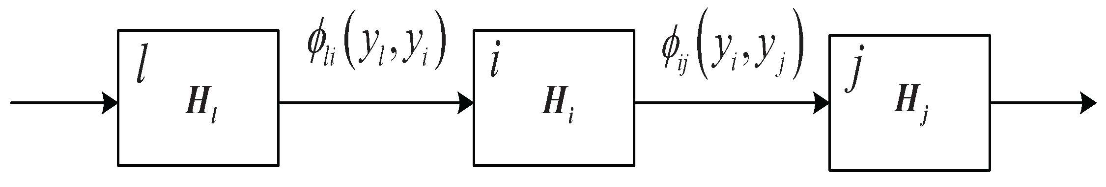
- Composition of hybrid automata. In , is the closed hybrid automaton over the digraph obtained by parallel composition of hybrid automata in , i.e., with and ; ; is defined as and describes the dynamics of vertex i by substituting in the the following equationwith the following relation:where denotes the projected subspace of S on the state components with indices in , and for any the output is given bytransition map is defined by the following rule:; ; .
3. DGHA Model For Urban Freeway Network
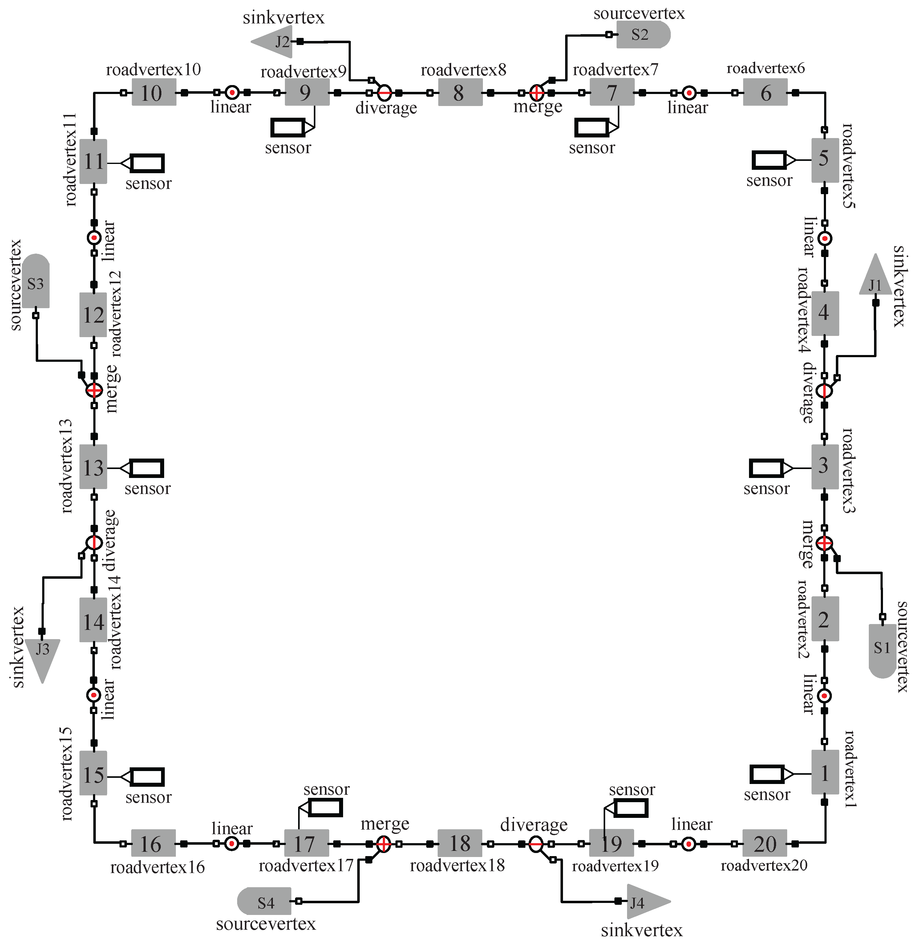
3.1. The Dual Digraph Description of Road Network
3.2. Dynamics of Traffic Flow in Road Segment
- , where , “, ”, and the continuous state space is since only density is adopted as continuous state variable;
- can be given arbitrarily;
- The input variable represents the changed flow of road segment i during the time period , where T is the sample time period. Thus we have the input space ;
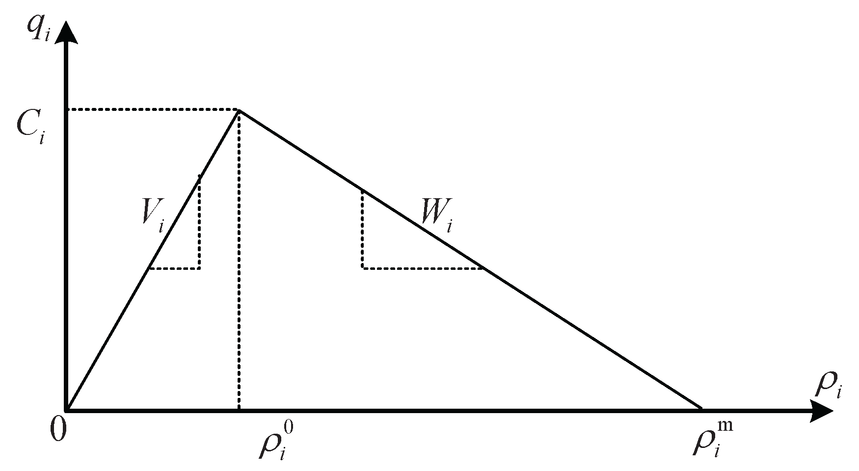
- The vector field is described by the following equation:where and is the length of the road segment (cell) i. Here and henceforth for simplicity we omit the time t in various variables and use to express ;
- The transition map is defined according to the guard conditions, i.e., a transition happens if and only if the corresponding invariant set is damaged and the guard condition is satisfied; The reset map is identical and thus is omitted;
- The invariant sets are and ;
- The guard conditions are and ;
- The output space is ;
- The output function is defined as , where is the flow that can be received by cell i over the interval ), is the flow that can be supplied by cell i over the interval ), i.e.,
3.3. Multi-Mode Description of Transited Traffic Flows
3.4. Composition for DGHA Model of Traffic Flow Network
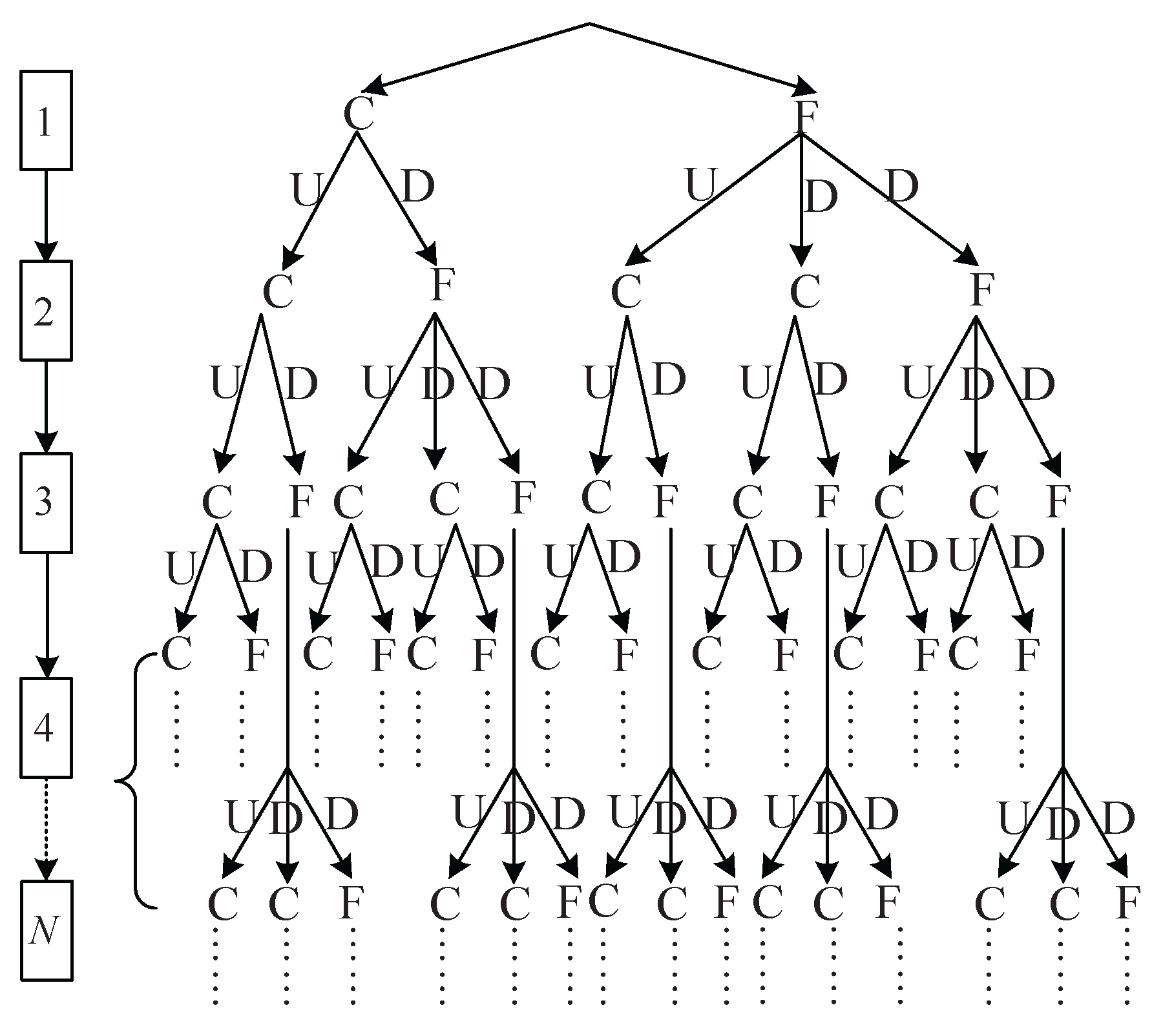
3.5. Analysis of the Number of Combined Modes
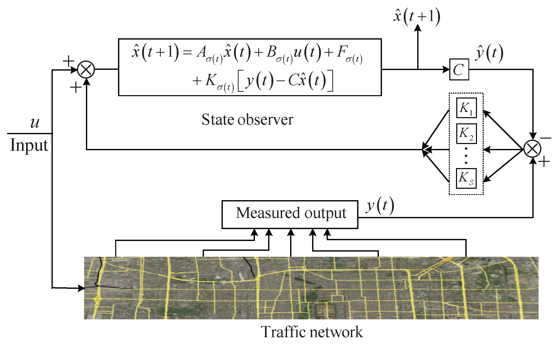
4. State Observer Design
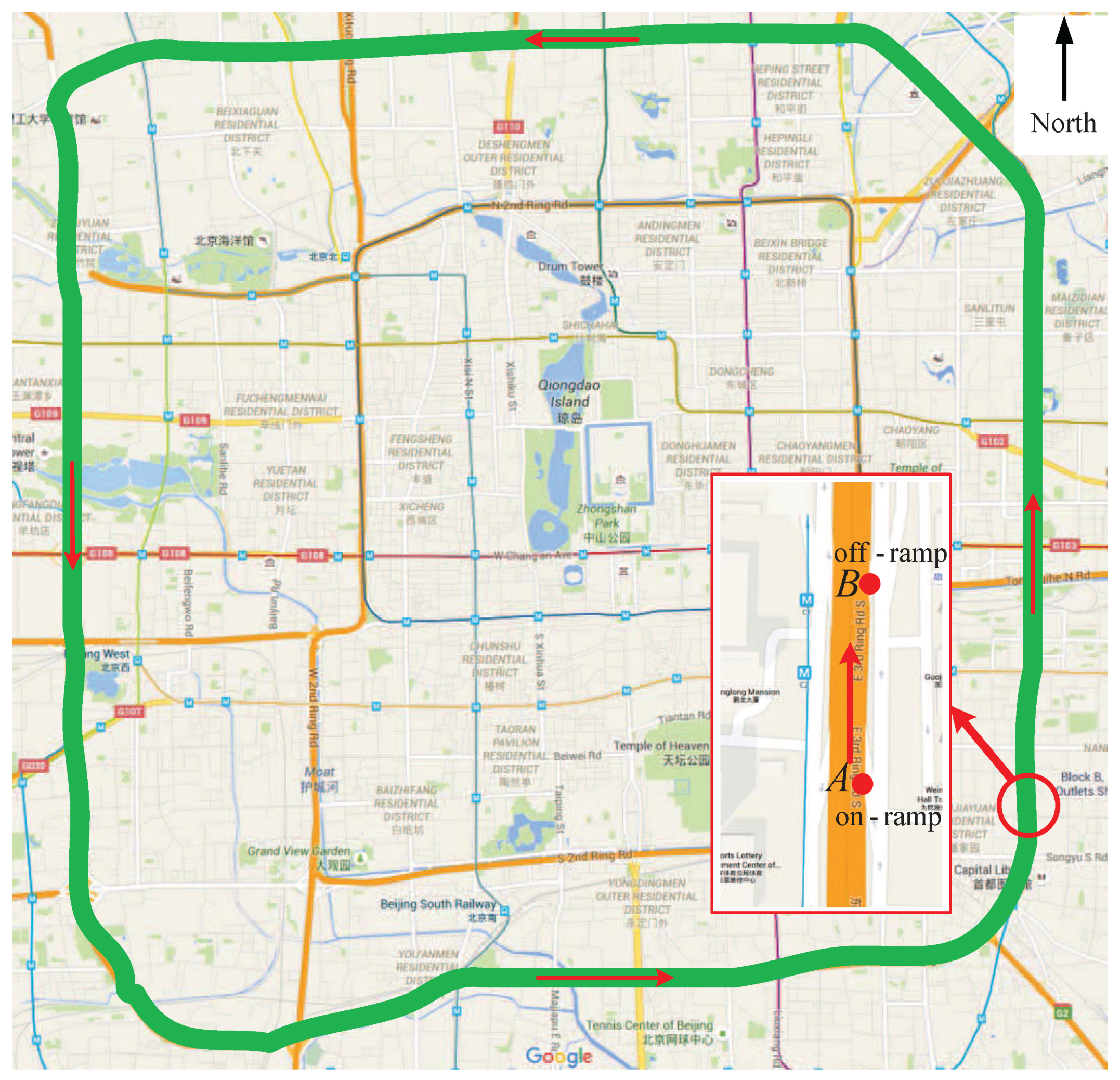
5. Application to Beijing Third Ring Freeway
5.1. Test Data and Parameter Settings
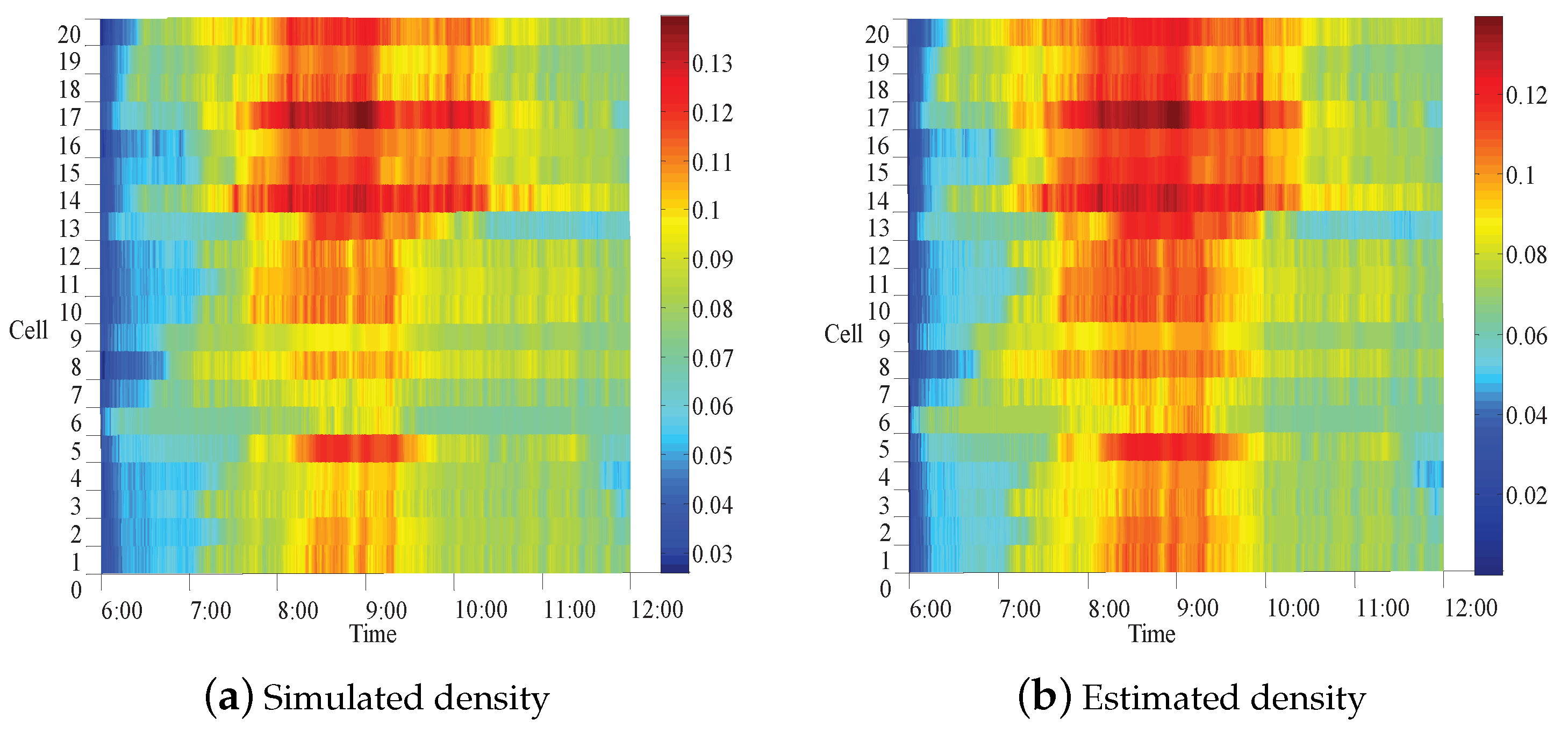
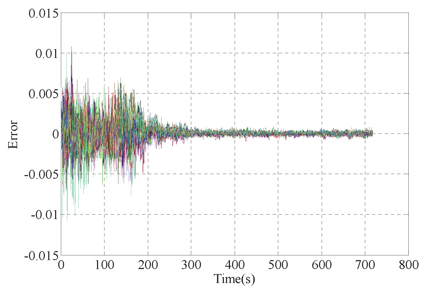
5.2. Analysis of Simulation Results
6. Conclusions and Future Work
Acknowledgments
Author Contributions
Conflicts of Interest
Appendix A
Appendix B
References
- Newman, M.E.J. The structure and function of complex networks. SIAM Rev. 2003, 45, 167–256. [Google Scholar] [CrossRef]
- Barrat, A.; Barthelemy, M.; Vespignani, A. Dynamical Processes on Complex Networks; Cambridge University Press: New York, NY, USA, 2008; pp. 242–264. [Google Scholar]
- Lighthill, M.J.; Whitham, G.B. On kinematic waves. II. A theory of traffic flow on long crowded roads. Proc. R. Soc. Lond. A Math. Phys. Eng. Sci. 1955, 229, 317–345. [Google Scholar] [CrossRef]
- Richards, P.I. Shock waves on the highway. Oper. Res. 1956, 4, 42–51. [Google Scholar] [CrossRef]
- Payne, H.J. Models of Freeway Traffic and Control; SIMULATION COUNCILS, INC.: San Diego, CA, USA, 1971; pp. 51–61. [Google Scholar]
- Daganzo, C.F. The cell transmission model: A dynamic representation of highway traffic consistent with the hydrodynamic theory. Transp. Res. Part B Methodol. 1994, 28, 269–287. [Google Scholar]
- Daganzo, C.F. The cell transmission model, part II: Network traffic. Transp. Res. Part B Methodol. 1995, 29, 79–93. [Google Scholar] [CrossRef]
- Lebacque, J.P. The Godunov scheme and what it means for first order traffic flow models. In Proceedings of the 13th Internaional Symposium on Transportation and Traffic Theory, Lyon, France, 24–26 July 1996; pp. 647–677. [Google Scholar]
- Flötteröd, G.; Nagel, K. Some practical extensions to the Cell Transmission Model. In Proceedings of the 2005 8th IEEE international Conference on Intelligent Transportation Systems(ITSC), Vienna, Austria, 13–16 September 2005; pp. 172–177. [Google Scholar]
- Gomes, G.; Horowitz, R. Globally optimal solutions to the on-ramp metering problem-Part I. In Proceedings of the 7th IEEE international Conference on Intelligent Transportation Systems(ITSC), Washington, DC, USA, 3–6 October 2004; pp. 509–514. [Google Scholar]
- Gomes, G.; Horowitz, R. Optimal freeway ramp metering using the asymmetric cell transmission model. Transp. Res. Part C Emerg. Technol. 2006, 14, 244–262. [Google Scholar] [CrossRef]
- Gomes, G.; Horowitz, R. Globally optimal solutions to the on-ramp metering problem-Part II. In Proceedings of the 7th IEEE international Conference on Intelligent Transportation Systems(ITSC), Washington, DC, USA, 3–6 October 2004; pp. 515–520. [Google Scholar]
- Lo, H.K. A cell-based traffic control formulation: strategies and benefits of dynamic timing plans. Transp. Sci. 2001, 35, 148–164. [Google Scholar] [CrossRef]
- Lin, W.H.; Wang, C. An enhanced 0-1 mixed-integer LP formulation for traffic signal control. IEEE Trans. Intell. Transp. Syst. (ITS) 2004, 5, 238–245. [Google Scholar] [CrossRef]
- Sumalee, A.; Zhong, R.; Pan, T.; Lam, W.H.K. Stochastic cell transmission model (SCTM): A stochastic dynamic traffic model for traffic state surveillance and assignment. Transp. Res. Part B Methodol. 2011, 45, 507–533. [Google Scholar]
- Canudas-de-Wit, C.; Ojeda, L.L.; Kibangou, A.Y. Graph constrained-CTM observer design for the Grenoble south ring. In Proceedings of the 13th IFAC Symposium on Control in Transportation Systems, Sofia, Bulgaria, 12–14 September 2012; Volume 45, pp. 197–202. [Google Scholar]
- Muñoz, L.; Sun, X.; Horowitz, R.; Luis, A. Piecewise-linearized cell transmission model and parameter calibration methodology. Transp. Res. Rec. 2006, 1965, 183–191. [Google Scholar]
- Muñoz, L.; Sun, X.; Horowitz, R.; Luis, A. Traffic density estimation with the cell transmission model. In Proceedings of the 2003 American Control Conference (ACC), Denver, CO, USA, 4–6 June 2003; Volume 5, pp. 3750–3755. [Google Scholar]
- Chen, Y.; He, Z.; Shi, J.; Han, X. Dynamic graph hybrid system: A modeling method for complex networks with application to urban traffic. In Proceedings of the 10th Intelligent Control and Automation (WCICA), Beijing, China, 6–8 July 2012; pp. 1864–1869. [Google Scholar]
- Chen, Y.; Li, W.; Guo, Y.; Wu, Y. Dynamic graph hybrid automata: A modeling method for traffic network. In Proceedings of the 18th IEEE international Conference on Intelligent Transportation Systems(ITSC), Canary Islands, Spain, 15–18 September 2015; pp. 1396–1401. [Google Scholar]
- Chen, Y.; Guo, Y.; Wang, Y.; Li, W. Modeling freeway network by using dynamic graph hybrid automata and estimating its states by designing state observer. In Proceedings of the Chinese Automation Congress (CAC), Wuhan, China, 27–29 November 2015; pp. 237–242. [Google Scholar]
- Sun, X.; Muñoz, L.; Horowitz, R. Mixture Kalman filter based highway congestion mode and vehicle density estimator and its application. In Proceedings of the American Control Conference (ACC), Boston, MA, USA, 30 June–2 July 2004; Volume 3, pp. 2098–2103. [Google Scholar]
- Harary, F.; Gupta, G. Dynamic graph models. Math. Comput. Model. 1997, 25, 79–87. [Google Scholar]
- Lunze, J.; Lamnabhi-Lagarrigue, F. Handbook of Hybrid Systems Control: Theory, Tools, Applications; Cambridge University Press: New York, NY, USA, 2009. [Google Scholar]
- Henzinger, T.A. The theory of hybrid automata. Verification of Digital and Hybrid Systems; Springer: Berlin/Heidelberg, Germany, 2000; pp. 278–292. [Google Scholar]
- Varaiya, P. Smart cars on smart roads: problems of control. IEEE Trans. Autom. Control 1993, 38, 195–207. [Google Scholar] [CrossRef]
- Lygeros, J.; Godbole, D.N.; Sastry, S. Verified hybrid controllers for automated vehicles. IEEE Trans. Autom. Control 1998, 43, 522–539. [Google Scholar]
- Lei, J.; Ozguner, U. Decentralized hybrid intersection control. In Proceedings of the 40th IEEE Conference on Decision and Control, Orlando, FL, USA, 4–7 December 2001; Volume 2, pp. 1237–1242. [Google Scholar]
- Zhao, X.; Chen, Y. Traffic light control method for a single intersection based on hybrid systems. In Proceedings of the 2003 IEEE Intelligent Transportation Systems, Shanghai, China, 12–15 October 2003; Volume 2, pp. 1105–1109. [Google Scholar]
- Zhao, X.; Chen, Y.; Li, Z.; Chen, Y. An optimal control method for hybrid systems based on Q-learning for an intersection traffic signal control. Chin. High Technol. Lett. 2007, 17, 498–502. [Google Scholar]
- Jiang, G.; Chen, Y.; Zhang, L.; Li, H.F. Modeling and Reachability Analysis for Single Intersection Based on Rectangular Hybrid Automata. J. Transp. Syst. Eng. Inf. Technol. 2009, 9, 120–126. [Google Scholar]
- Grahlmann, B. Combining finite automata, parallel programs and SDL using petri nets. In Proceedings of the International Conference on Tools and Algorithms for the Construction and Analysis of Systems; Springer: Berlin/Heidelberg, Germany, 1998; pp. 102–117. [Google Scholar]
- Uygur, G.; Sattler, S.M. Parallel Composition-A practical solution. In Proceedings of the 1st International Electric Drives Production Conference (EDPC), Nuremberg, Germany, 28–29 September 2011; pp. 235–242. [Google Scholar]
- Rinaldi, M.; Capisani, L.; Ferrara, A.; Nunez, A.; Hajiahmadi, M.; De Schutter, B. Distributed identification of the cell transmission traffic model: A case study. In Proceedings of the American Control Conference (ACC), Montréal, QC, Canada, 27–29 June 2012; pp. 6545–6550. [Google Scholar]
- Vigos, G.; Papageorgiou, M.; Wang, Y. Real-time estimation of vehicle-count within signalized links. Transp. Res. Part C Emerg. Technol. 2008, 16, 18–35. [Google Scholar] [CrossRef]
- Wang, Y.; Papageorgiou, M. Real-time freeway traffic state estimation based on extended Kalman filter: A general approach. Transp. Res. Part B Methodol. 2005, 39, 141–167. [Google Scholar] [CrossRef]
- Anand, A.; Ramadurai, G.; Vanajakshi, L. Data fusion-based traffic density estimation and prediction. J. Intell. Transp. Syst. 2014, 18, 367–378. [Google Scholar] [CrossRef]
- Mihaylova, L.; Boel, R.; Hegyi, A. Freeway traffic estimation within particle filtering framework. Automatica 2007, 43, 290–300. [Google Scholar] [CrossRef]
- Kurzhanskiy, A.A.; Varaiya, P. Guaranteed prediction and estimation of the state of a road network. Transp. Res. Part C Emerg. Technol. 2012, 21, 163–180. [Google Scholar] [CrossRef]
- Kurzhanskiy, A.A. Set-valued estimation of freeway traffic density. In Proceedings of the IFAC Symposium on Transportation Systems, Redondo Beach, CA, USA, 2–4 September 2009; Volume 42, pp. 271–277. [Google Scholar]
- Kurzhanskiy, A.A.; Varaiya, P. Active traffic management on road networks: A macroscopic approach. Philos. Trans. R. Soc. Lond. A Math. Phys. Eng. Sci. 2010, 368, 4607–4626. [Google Scholar] [CrossRef] [PubMed]
- Alessandri, A.; Coletta, P. Design of Luenberger observers for a class of hybrid linear systems. In Proceedings of the International Workshop on Hybrid Systems: Computation and Control, Rome, Italy, 28–30 March 2001; Volume 2034, pp. 7–18. [Google Scholar]
- Alessandri, A.; Coletta, P. Switching observers for continuous-time and discrete-time linear systems. In Proceedings of the American Control Conference (ACC), Arlington, VA, USA, 25–27 June 2001; Volume 3, pp. 2516–2521. [Google Scholar]
- Bara, G.I.; Daafouz, J.; Kratz, F.; Iung, C. State estimation for a class of hybrid systems. In Proceedings of the 4th International Conference on Automation of Mixed Processes, Dortmund, Germany, 18–19 September 2000; pp. 313–316. [Google Scholar]
- Juloski, A.L.; Heemels, W.; Weiland, S. Observer design for a class of piece-wise affine systems. In Proceedings of the 41st IEEE Conference on Decision and Control, Las Vega, NV, USA, 10–13 December 2002; Volume 3, pp. 2606–2611. [Google Scholar]
- Juloski, A.L.; Heemels, W.; Boers, Y.; Verschure, F. Two approaches to state estimation for a class of piecewise affine systems. In Proceedings of the 42nd IEEE Conference on Decision and Control, Maui, HI, USA, 9–12 December 2003; Volume 1, pp. 143–148. [Google Scholar]
- Tanwani, A.; Shim, H.; Liberzon, D. Observability for switched linear systems: Characterization and observer design. IEEE Trans. Autom. Control 2013, 58, 891–904. [Google Scholar] [CrossRef]
- Pettersson, S. Observer design for switched systems using multiple quadratic Lyapunov functions. In Proceedings of the IEEE International Symposium on Intelligent Control, Limassol, Cyprus, 27–19 June 2005; pp. 262–267. [Google Scholar]
- Pettersson, S. Designing switched observers for switched systems using multiple Lyapunov functions and dwell-time switching. In Proceedings of the 2nd IFAC Conference on Analysis and Design of Hybrid Systems, Alghero, Italy, 7–9 June 2006; Volume 39, pp. 18–23. [Google Scholar]
- Gómez-GutiÉrrez, D.; Čelikovský, A.; Ramĺrez-Trevinños, A.; Castillo-Toledo, B. On the observer design problem for continuous-time switched linear systems with unknown switchings. J. Frankl. Inst. 2015, 352, 1595–1612. [Google Scholar] [CrossRef]
- Morbidi, F.; Ojeda, L.L.; Canudas-de-Wit, C.; Bellicot, I. A new robust approach for highway traffic density estimation. In Proceedings of the European Control Conference (ECC), Strasbourg, France, 24–27 June 2014; pp. 2575–2580. [Google Scholar]
- Alvarez-Icaza, L.; Muñoz, L.; Sun, X.; Horowitz, R. Adaptive observer for traffic density estimation. In Proceedings of the American Control Conference, Boston, MA, USA, 30 June–2 July 2004; pp. 2705–2710. [Google Scholar]
- Castillo, E.; Conejo, A.J.; Menéndez, J.M.; Jiménez, P. The observability problem in traffic network models. Comput. Aided Civ. Infrastruct. Eng. 2008, 23, 208–222. [Google Scholar] [CrossRef]
- Castillo, E.; Jiménez, P.; Menéndez, J.M.; Conejo, A.J. The observability problem in traffic models: Algebraic and topological methods. IEEE Trans. Intell. Transp. Syst. 2008, 9, 275–287. [Google Scholar] [CrossRef]
- Agarwal, S.; Kachroo, P.; Contreras, S. A dynamic network modeling-based approach for traffic observability problem. IEEE Trans. Intell. Transp. Syst. 2016, 17, 1168–1178. [Google Scholar]
- Agarwal, S.; Kachroo, P.; Contreras, S.; Sastry, S. Feedback-coordinated ramp control of consecutive on-ramps using distributed modeling and Godunov-based satisfiable allocation. IEEE Trans. Intell. Transp. Syst. 2005, 16, 2384–2392. [Google Scholar]
- Navarro-Lopez, E.M.; Carter, R. Hybrid automata: An insight into the discrete abstraction of discontinuous systems. Int. J. Syst. Sci. 2011, 42, 1883–1898. [Google Scholar] [CrossRef]
- Boriboonsomsin, K.; Barth, M. Impacts of freeway high-occupancy vehicle lane configuration on vehicle emissions. Transp. Res. Part D Transp. Environ. 2008, 13, 112–125. [Google Scholar] [CrossRef]


| Mode | Condition of | Flow |
|---|---|---|
| FDF | ||
| FUF | ||
| CDF/CUF | ||
| CDC | ||
| CUC | ||
| FUC | ||
| FDC |
| Number | Length | Number | Length | Number | Length |
|---|---|---|---|---|---|
| 1 | 111 m | 8 | 430 m | 15 | 300 m |
| 2 | 535 m | 9 | 500 m | 16 | 350 m |
| 3 | 336 m | 10 | 355 m | 17 | 332 m |
| 4 | 138 m | 11 | 338 m | 18 | 210 m |
| 5 | 586 m | 12 | 355 m | 19 | 367 m |
| 6 | 140 m | 13 | 458 m | 20 | 458 m |
| 7 | 281 m | 14 | 256 m |
| Number | V | W | C | ||
|---|---|---|---|---|---|
| 2,3,4 | 65 | 20 | 2800 | 46 | 185 |
| 7,8,9 | 63 | 21 | 2850 | 45 | 180 |
| 12,13,14 | 65 | 20 | 2760 | 44 | 182 |
| 17,18,19 | 62 | 19 | 2650 | 43 | 180 |
| 1,20 | 60 | 19 | 2450 | 40 | 170 |
| 5,6 | 58 | 18 | 2350 | 41 | 165 |
| 10,11 | 55 | 20 | 2200 | 40 | 150 |
| 15,16 | 50 | 19 | 2100 | 41 | 155 |
| Number of cell | 1 | 2 | 3 | 4 | 5 | 6 | 7 | 8 | 9 | 10 |
| MSE | 0.1095 | 0.1126 | 0.1132 | 0.1223 | 0.1205 | 0.1176 | 0.1301 | 0.1005 | 0.1108 | 0.1201 |
| Number of cell | 11 | 12 | 13 | 14 | 15 | 16 | 17 | 18 | 19 | 20 |
| MSE | 0.1132 | 0.1087 | 0.1136 | 0.1009 | 0.1143 | 0.1209 | 0.1120 | 0.1013 | 0.1147 | 0.1106 |
© 2017 by the authors. Licensee MDPI, Basel, Switzerland. This article is an open access article distributed under the terms and conditions of the Creative Commons Attribution (CC BY) license (http://creativecommons.org/licenses/by/4.0/).
Share and Cite
Chen, Y.; Guo, Y.; Wang, Y. Modeling and Density Estimation of an Urban Freeway Network Based on Dynamic Graph Hybrid Automata. Sensors 2017, 17, 716. https://doi.org/10.3390/s17040716
Chen Y, Guo Y, Wang Y. Modeling and Density Estimation of an Urban Freeway Network Based on Dynamic Graph Hybrid Automata. Sensors. 2017; 17(4):716. https://doi.org/10.3390/s17040716
Chicago/Turabian StyleChen, Yangzhou, Yuqi Guo, and Ying Wang. 2017. "Modeling and Density Estimation of an Urban Freeway Network Based on Dynamic Graph Hybrid Automata" Sensors 17, no. 4: 716. https://doi.org/10.3390/s17040716
APA StyleChen, Y., Guo, Y., & Wang, Y. (2017). Modeling and Density Estimation of an Urban Freeway Network Based on Dynamic Graph Hybrid Automata. Sensors, 17(4), 716. https://doi.org/10.3390/s17040716