4.1. Fuzzy C-Means Clustering
Clustering and anomaly detection are extensively studied for trajectory mining applications [
1,
26]. Furthermore, the two techniques are often used in conjunction [
27]. In our project, we first cluster the arrival data into a trajectory fragment if those data should be grouped into the same route for a bus. Then, the anomaly detection method is applied to check whether there exist outliers in the trajectory fragment and removes the erroneous data according to the contextual relationship of the data. We adopt fuzzy C-means clustering (FCM) as the trajectory clustering method. FCM is a soft clustering method and was proposed by Bezdek [
28]. In the FCM method, the data
are partitioned into
c fuzzy sets by minimizing the objective function as follows:
where
is the fuzzification coefficient,
V is the prototype matrix with
denoting the
j-th cluster prototype,
U is the partition matrix with
denoting the membership value for
classified to cluster
j and
is a distance function. Usually, the Euclidean distance is considered for
. The membership
is constrained by:
The minimization of
with Constraint (
2) gives [
28]:
In practice, the partition matrix
U and prototype matrix
V are updated in an iterative way by Formulas (
3) and (
4) until the change of objective function
between two consecutive iteration is less than a predefined tolerance or the maximum iterating times reached.
In this paper, we utilize the FCM method to cluster the arrival data with the objective that the data in the same cluster should belong to the same route. Of course, the best result is one cluster for one-route trajectory. However, due to the disturbance of outliers and data missing problems, the actual clusters are not always equal to the route trajectories.
4.2. Feature Construction for FCM
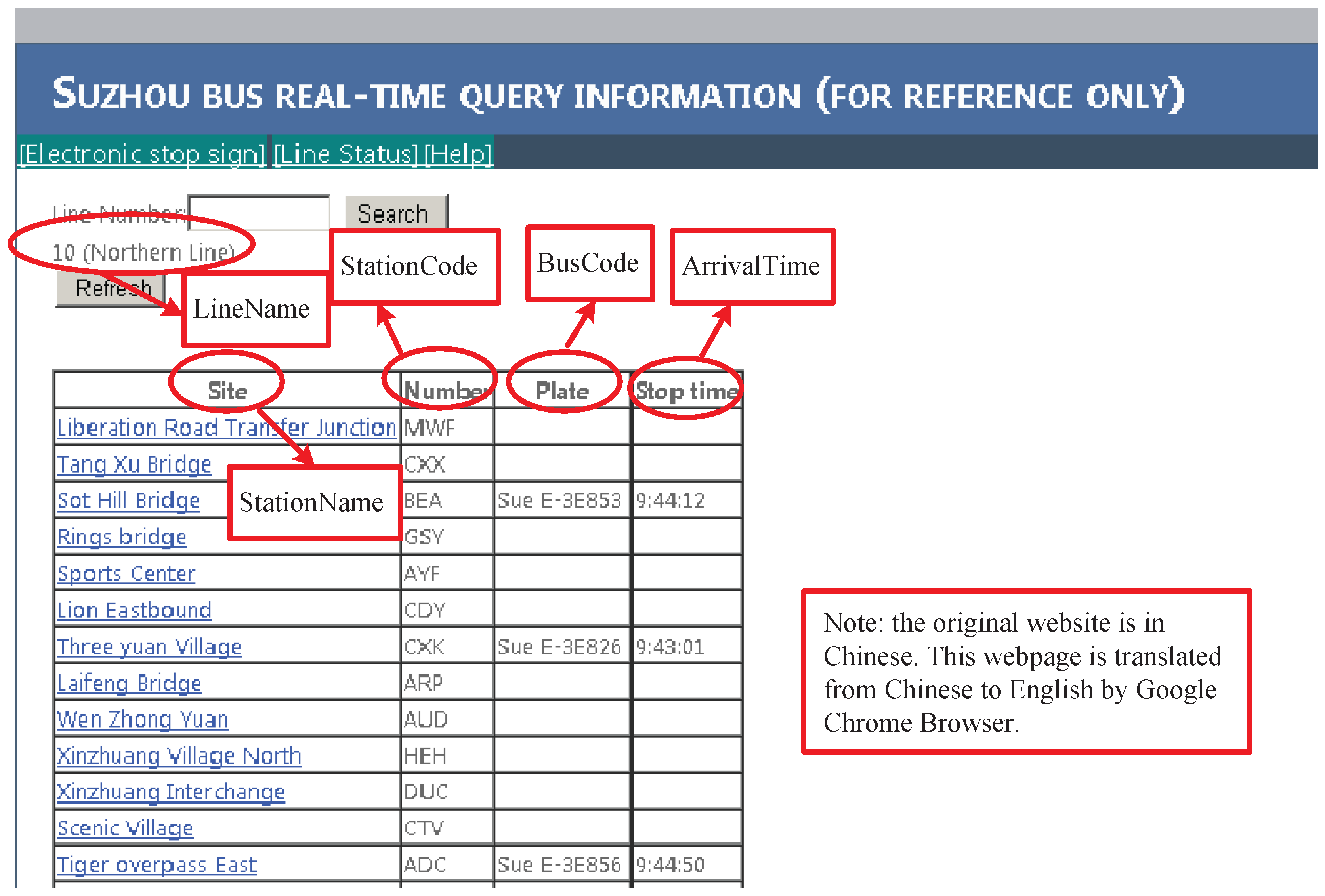
Feature construction is an important work in FCM. The arrival data contains three-dimensional information generated by line l. Usually, one line consists of several buses that can be distinguished by in . In the sense of trajectory clustering, we wish to partition the arrival data generated by one route in into one cluster. Hence, the arrival data generated by different buses should be naturally partitioned into different trajectory clusters. However, if we take as the input feature of X for FCM, the distance for cannot effectively measure the difference between different trajectories. On the other hand, the two-dimensional information extracted from is better for trajectory clustering, since all arrival data in are generated by the same bus m, and arrival data generated by different buses are naturally separated by with different values of m. In practice, there are more abnormal arrival data at the first and final stations than other stations; we eliminate the FF-data (arrival data of the first and final stations) before trajectories extraction for the sake of reducing the negative effect introduced by abnormal data.
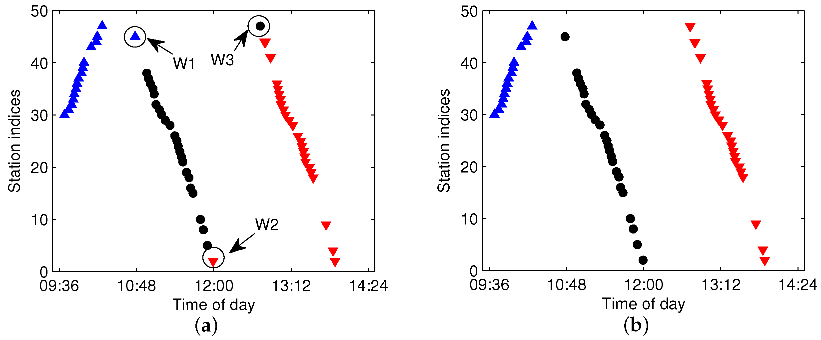
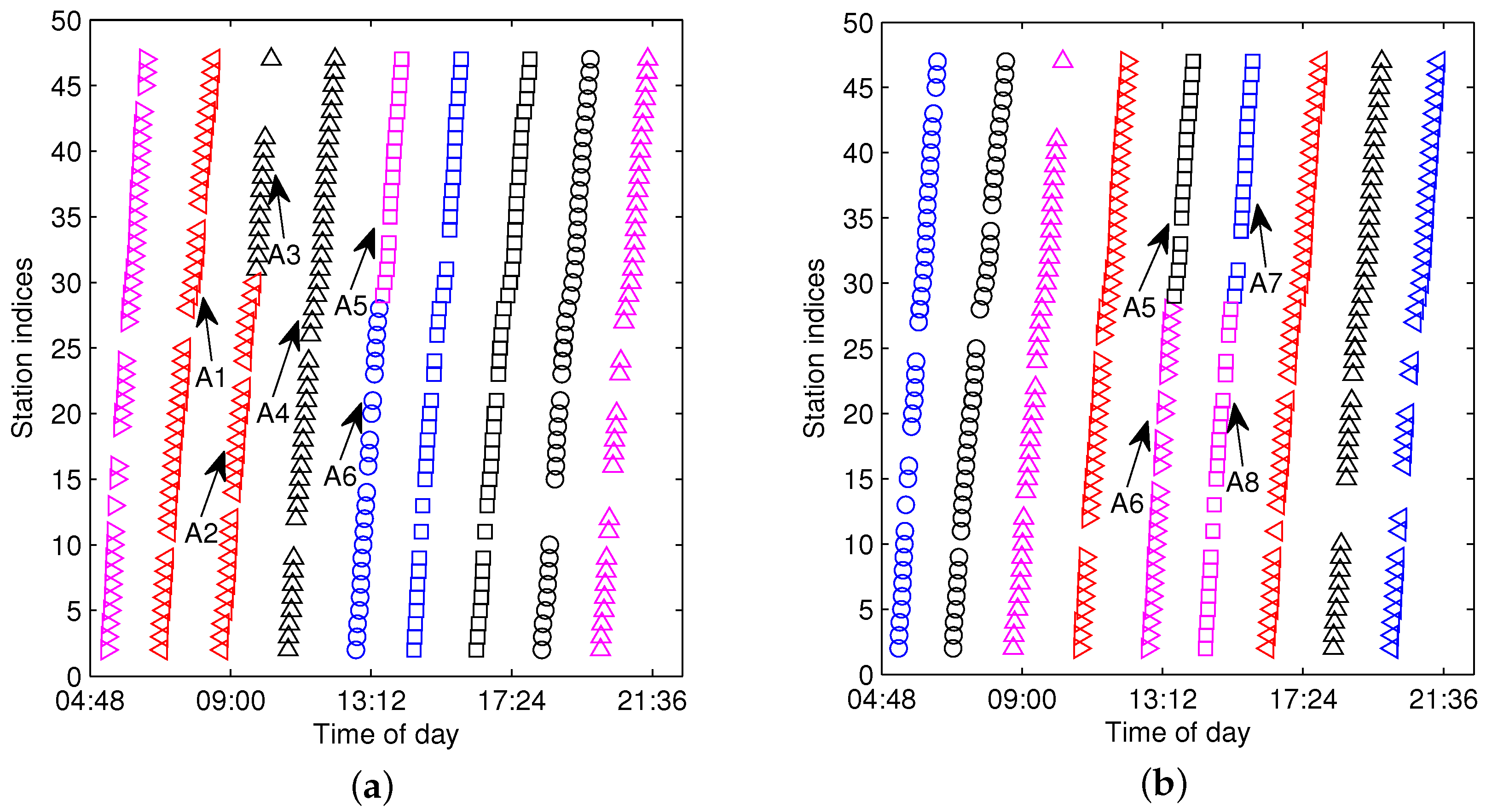
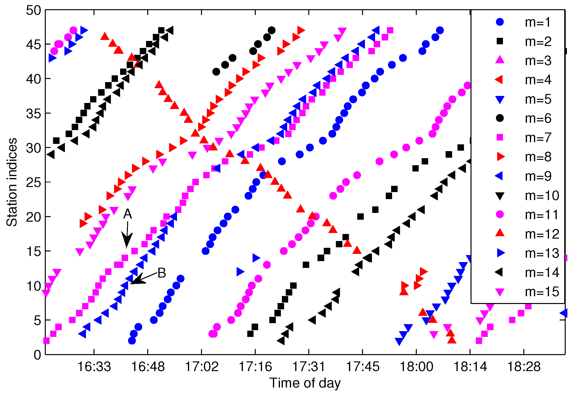
Figure 6 shows the arrival events grouped by
after eliminating the FF-data for the same dataset shown in
Figure 4. As illustrated in
Figure 6, Trajectories A and B can be efficiently distinguished by
; however, quite differently, they are difficult to partition from
without the bus-code information when the trajectories are in a short headway or bunched, as shown in
Figure 4. If we adopt the method presented in [
15], Trajectories A and B will not be extracted correctly. Hence, grouping arrival data by
instead of
is a sensible choice for the purpose of trajectory extraction, especially for the trajectories in a short headway. Though
can separate trajectories from different buses, the arrival data in
still consist of several traveling routes and need to be further partitioned from each other.
The FCM clustering of
is aimed to separate the arrival data by one cluster for each one-route trajectory.
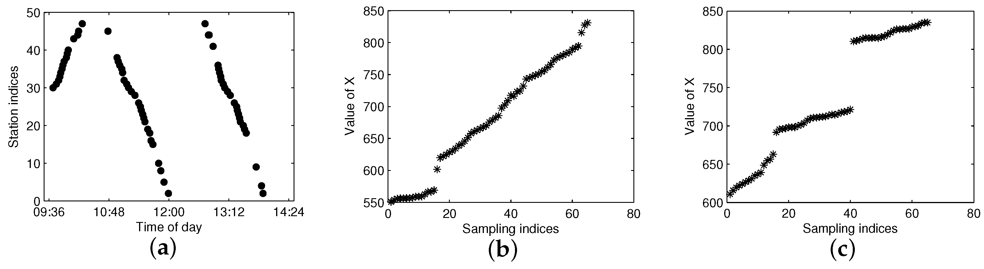
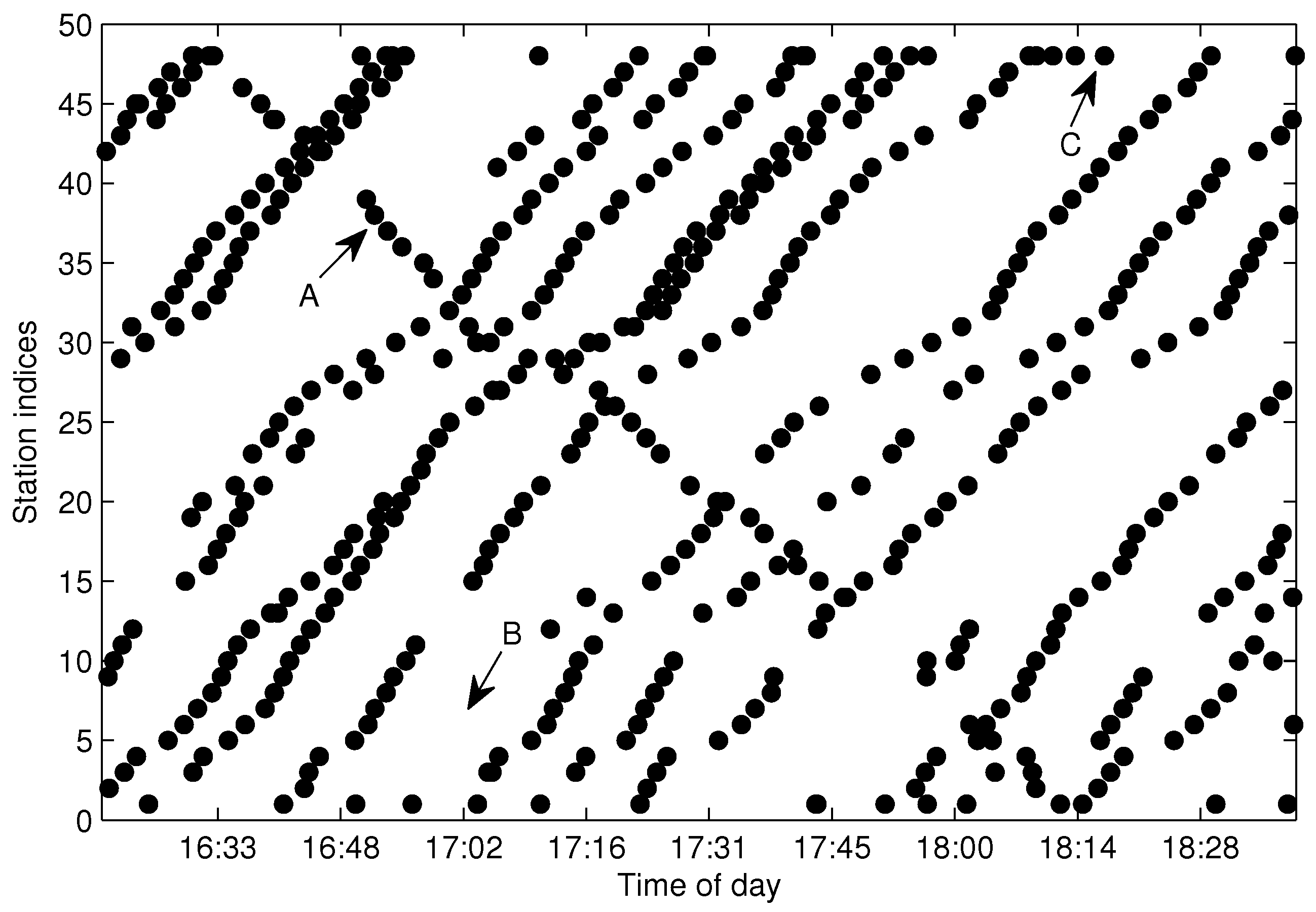
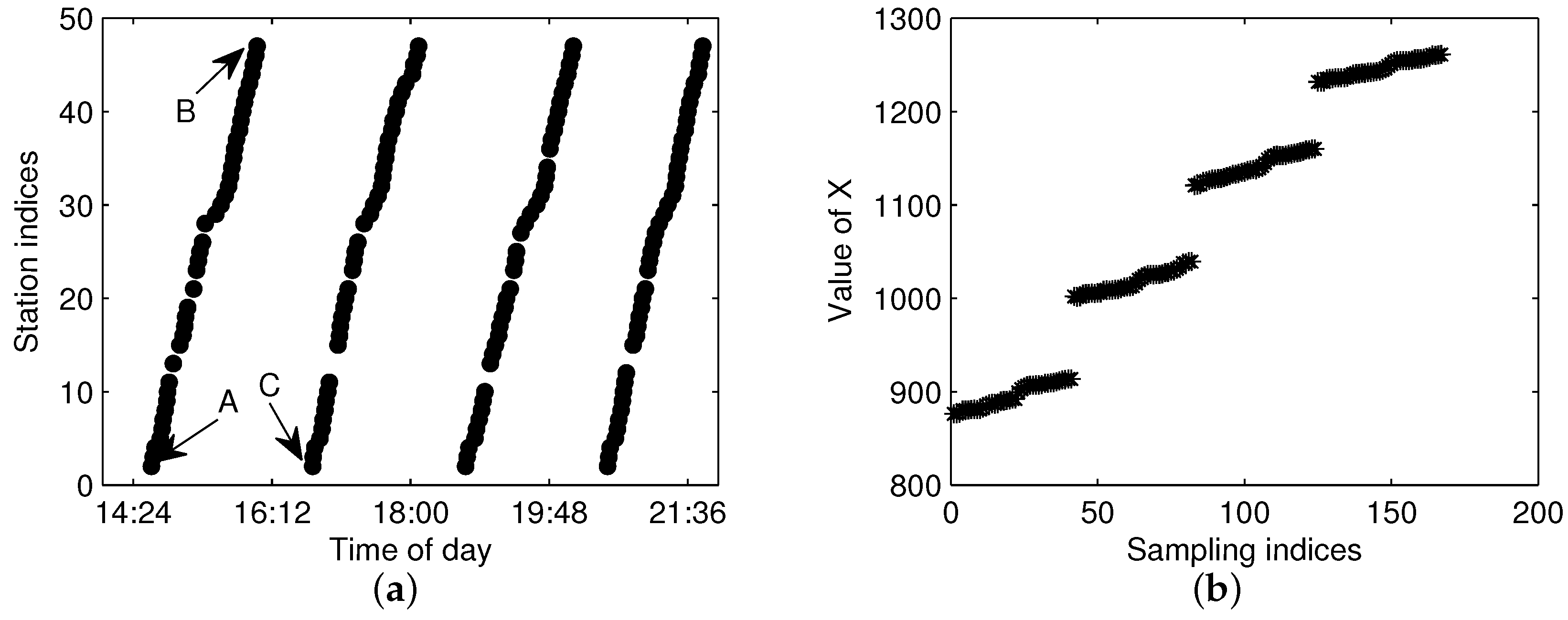
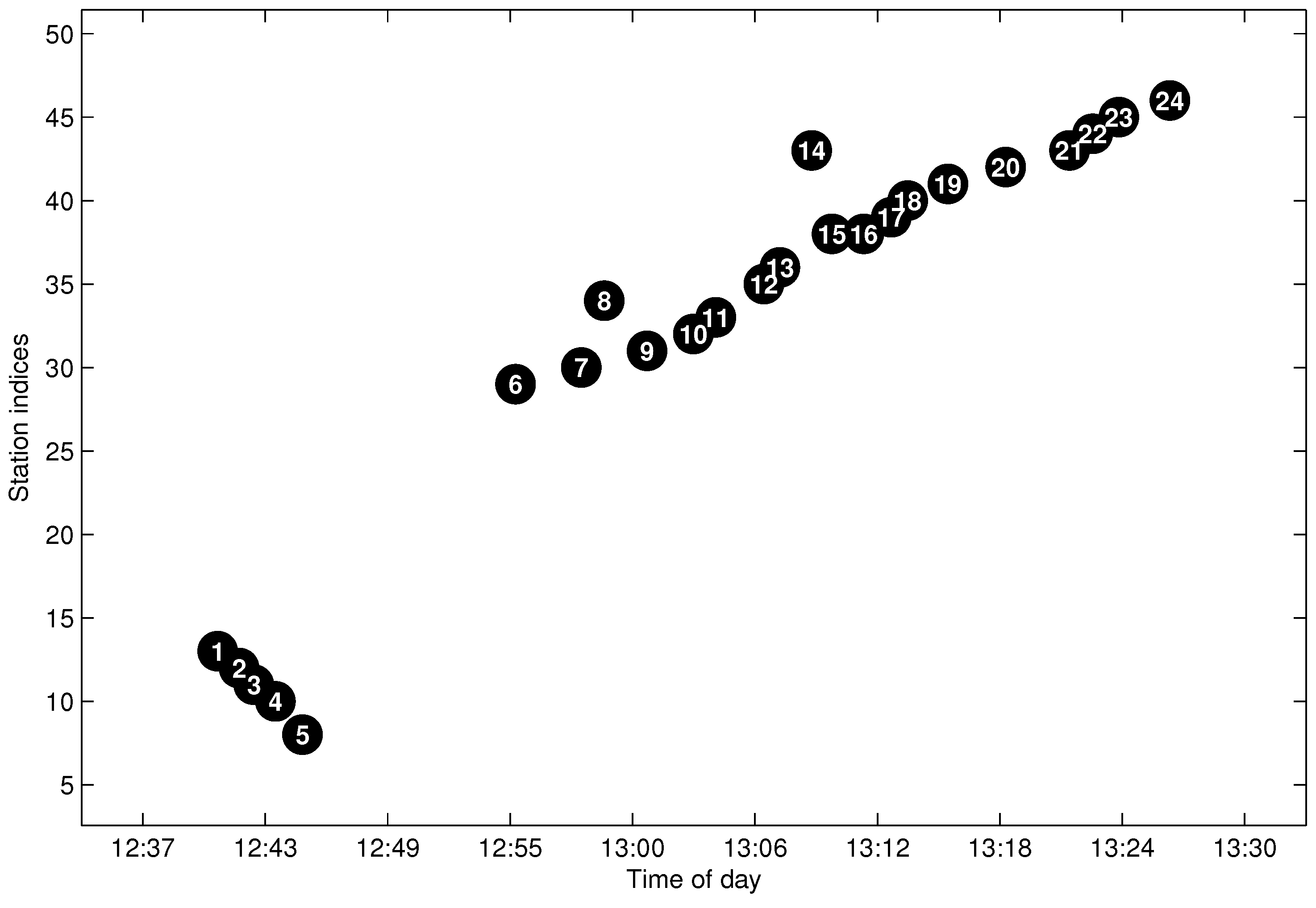
Figure 7a shows the arrival events by the bus with
for the same line and sampling date as in
Figure 4. From the figure, one can see that there are total of four traveling routes for bus
, which means that the work of trajectory extraction is to extract the four trajectories and add them into
. The first problem for FCM is how to measure the distance of trajectory data in order to get a large distance between different trajectories and a small distance in the same trajectory. Though traditional Euclidean distance is widely used in clustering, it is not a good metric for our FCM clustering. We take three points in
Figure 7a as an example, as shown in the figure, Points
A and
B are in the same trajectory; however, the Euclidean distance between
A and
C (points from different trajectories) is smaller than the distance between
A and
B, which will result in the wrong clustering for FCM.
For trajectory clustering by FCM, we construct an enhanced distance metric by considering the traveling time along the route direction. Let the
j-th record in
be
; then, the input feature
for
is:
where
is the arrival time for record
j,
is the arrival station index in line
l and
is a linear function of the traveling time from the first station to station
. For most stations in the studied city, the uncongested traveling time between two consecutive stations is about 2 min, and
is selected as half of the traveling time; hence, a robust and convenient choice for the initial value of
is:
Once the trajectories of a studied line are extracted,
can be refined according to the historical traveling time derived from the trajectories.
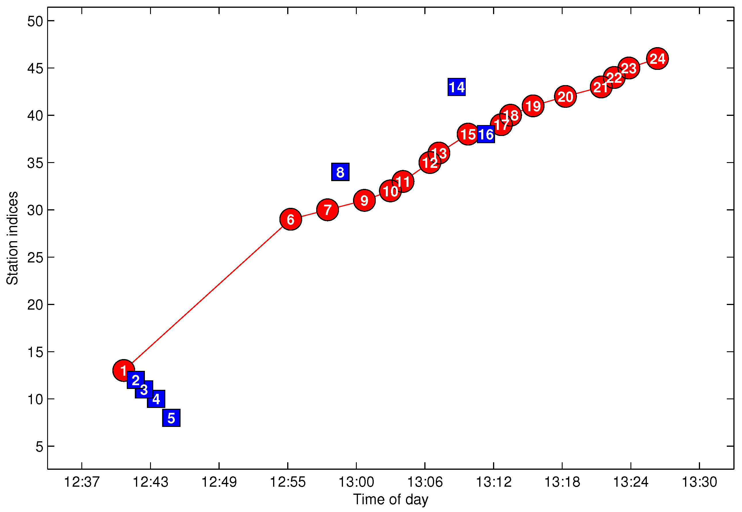
Figure 7b shows the constructed input feature
X of
. As shown in the figure, the constructed
X is a one-dimensional datum, which can split the traveling data of
into four clusters well, with each cluster mapped to a one-route trajectory. The illustrated case in
Figure 7 is suitable for the well-conditioned traveling data without noise. However, there may exist some abnormal data as depicted in
Figure 4; the input feature constructed by Equations (
5) and (
6) thus may reduce the separable performance when the arrival data in
contain more trajectories in the opposite direction than those in the correct direction. In order to enhance the separability for the case of the wrong direction trajectories, the
in Equation (
6) is modified by:
and
in Equation (
5) is modified as:
The
X constructed by Equation (
5) is called the forward clustering feature, and the one constructed by Equation (
8) is called the backward clustering feature in this paper. Accordingly, we call the fuzzy C-means clustering with the forward clustering feature as forward FCM (F-FCM) and the one with backward clustering feature as backward FCM (B-FCM).
4.3. Parameters Selection for FCM
The most important parameters for our trajectory extraction in the procedure of FCM are the number of fuzzy sets
c and initial prototypes. In practice, the counts of trajectories always change by different buses in different sampling days and need to be determined automatically. We count the trajectories based on station scanning, which is depicted as follows:
where
is the count of trajectories for
,
N is the number of stations in line
l,
is the size of the set and
is defined in Definition 3. Since there are more abnormal arrival events at the first and final stations, the scanning process is started from the second station and terminated before the final station to reduce the effect of outliers. Actually, the scanned
may be less than the actual count (denoted by
) in some cases caused by data missing or be greater than
in other cases caused by over-reporting. We prefer to set
to avoid partitioning two different trajectories into one cluster. In our extraction procedure,
c is set by:
where
is the gain of
c over
and is chosen by
in most cases. In Equation (
10),
is an integer operation rounding
to the nearest integer less than or equal to
.
The iterative algorithm for FCM clustering is a local optimization procedure; hence, different initial prototypes may result in different partitions. One property of the constructed feature
X is that both
X and trajectories are ordered in arrival time. Inspired by the time-ordered property, we proposed an initial prototype selection method as follows:
where
is the
i-th prototype in the initial prototype vector
,
is the
k-th element in
X and
c is the number of clusters. If all clusters are of the same size, the prototypes selection approach proposed in Equation (
11) will choose the center of the cluster as the initial prototype, which will reduce the clustering iterations. In this sense, the proposed initial prototypes selection method is better than random selection with the advantage that it costs less iterations in most cases when the sizes of the sampled trajectories are nearly equal.
4.5. Trajectory Fragment Cleaning
The aggregated from by FCM is called the trajectory fragments set in this paper. When the trajectory fragments set is generated by Algorithm 2, the following procedure is about outlier elimination, which is also called trajectory fragment cleaning in this paper.
We utilize fuzzy membership function (MF) to describe the relationship of arrival data in a trajectory, i.e., the introduced MF in our AD procedure describes the connecting possibility between two arrival events
and
to be classified into the same trajectory. In fuzzy set theory, most common membership functions are triangular, trapezoidal, Gaussian and bell-shaped [
29,
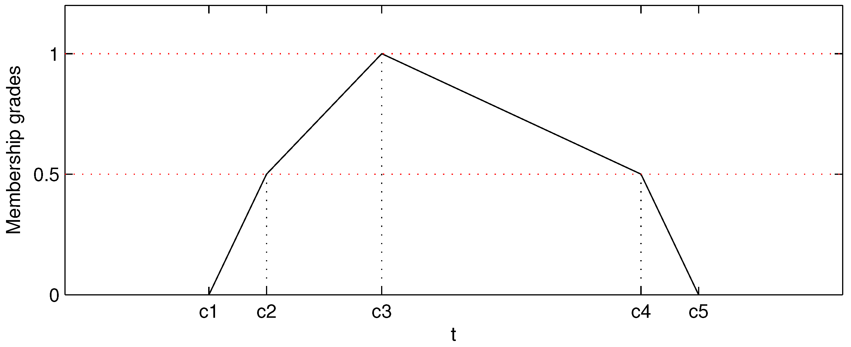
30]. In a more generalized viewpoint, the triangular and trapezoidal functions are in the forms of polygons, which are described by three parameters for the triangular and four parameters for the trapezoidal. In this paper, we extend the triangular to pentagonal MF, which is depicted as follows:
where
is the fuzzy MF of two arrival events to be connected into one trajectory and
are the five parameters describing the shape of pentagonal MF as shown in
Figure 8. For connecting possibility evaluation, the
t in Equation (
12) is the directional station-unit traveling time between
and
, which is calculated as follows:
where
and
.
If the trajectories for the studied lines have already been extracted, we can utilize the historical traveling time
t to determinate the parameters of the pentagonal MF by:
where
is the lower bound coefficient and
is the upper bound coefficient, which control the extended range of
t. Compared with the triangular MF, the pentagonal MF has the benefits of more flexible slope control. For data-based knowledge,
should be in high connecting possibility (
) for all
t in the historical data, and
(the highest connecting possibility) when
t is the median of the historical data. Moreover, the historical data cannot reveal all cases in the future, so the data range should be extended from historical data to make a better coverage for the future. Furthermore, the extensions are not symmetric for the lower bound and upper bound. The shortest traveling time is restricted by the highest vehicle velocity and distance between two stations, which can be expected once the shortest distance between two adjacent stations is given. Hence, there is a slight difference between
derived by historical data and the actual one in the future. However, the longest traveling time will be affected by traffic jam, traffic accident and other factors, which should be evaluated in a more conservative way. Actually, the
t in Equation (
13) is dependent on bus lines, station indices, date types and time of day. For the trajectory extraction work, it is hard to consider all of the factors when extracting hundreds of lines with millions of arrival events generated in one day. We prefer to evaluate
for all arrival events with a set of empirical parameters, which is given as follows:
where the
n-th row of
refers to the parametrical set of
with
in Equation (
13) and the
j-th column of
is the parameter
in Equation (
12). When
exceeds the maximum row index of
, the parameters for evaluating
are selected by the last row of
. By using
given in Equation (
15), the
between any two arrival events in a trajectory can be evaluated.
Let be the fuzzy connecting MF matrix evaluated for a trajectory fragment with N arrival events, where is the between the i-th and k-th arrival data when or when .
Let
be the cleaned trajectory fragment from
and
the cleaned fuzzy connecting MF matrix generated from
. We take the trajectory fragment cleaning as an optimization problem as follows:
where
is the size of
,
is the average of the elements in
and
is the connecting possibility threshold, which is given by empirical knowledge. We set
for all arrival data in the project. For a cleaned trajectory fragment
, every arrival datum in
should be connected, so all of the elements in
should be greater than the predefined threshold
. On the other hand, any data in
should not be misclassified as noisy data, which is guaranteed by the maximization of
.
Let be the anomalous indexing of the i-th data in , which is the count of satisfying for , and the anomalous indexing vector generated by .
Let be the set of the cleaned trajectory fragments.
Let be the noisy dataset generated from by the trajectory fragment cleaning algorithm, and . By the definition, one gets , and .
The solution of Problem (
16) is started by checking the noisy data with maximum anomalous indexing and deleting it from
recursively. The detailed solution of Problem (
16) is given by Algorithm 3.
| Algorithm 3 Trajectory fragment cleaning algorithm. |
| Input: , , ; |
| Output: , , ; |
Process:(a1) set a temporary noisy set ; (a2) get of with ; (a3) get from with ; if then go to (a5); else go to (a4); end if (a4) find the index k in with the maximum anomalous indexing; if k is not unique then choose be the one in k with the minimum row summation; else set ; end if update by adding the -th data in into ; delete the -th data in , delete the -th row and -th column in ; go to (a3); (a5) output the cleaned trajectories: if then set , and ; else set , and ; end if set .
|
4.6. Trajectory Fragments Connecting
In some cases, the one-route trajectory may be broken into two or more trajectory fragments. Hence, when generating
from
, some trajectories need to be connected to form a one-route trajectory. The process of generating
from
is named trajectory fragments connecting (TFC) in this paper. We introduce the fuzzy connecting matrix
for the processing of TFC. We denote
as the
i-th row and
j-th column element in
, which is defined as follows:
where
,
is the fuzzy connecting MF matrix generated from
,
is the cleaned trajectory from
and
is the average value of the elements in
.
and
are generated by Algorithm 3 for the input
. Rule 1 is described as follows:
where
is the size of noisy dataset
generated from
by Algorithm 3,
is the predefined parameter to control the maximum number of noisy data when considering
and
might be connected and
is as defined in Problem (
16). We set
in most cases for the TFC processing. In Constraint (
18),
is ahead of
in
, which means that all of the arrival events belonging to
in
happen before the other events in
. From Equation (
17) and Constraint (
18), one can see that
is not a symmetric matrix; moreover, if
, we will definitely have
.
In the processing of TFC, it is better to select the pair of fragments in with the maximum connecting possibility for connection, which is easily conducted by finding (the maximum element in ). Once and can be connected, we set and delete in . In this way, is partly updated in each connection round. The detail of TFC is given by Algorithm 4.
| Algorithm 4 Trajectory fragments connecting. |
| Input: , , ; |
| Output: ; |
Process:(a1) get of by Equation ( 17); (a2) if , go to (a4); (a3) find ; update by setting ; delete ; update by: recalculating the i-th row of ; removing both the j-th row and j-th column of ; goto (a2); (a4) set .
|
4.7. Missing Data Recovery
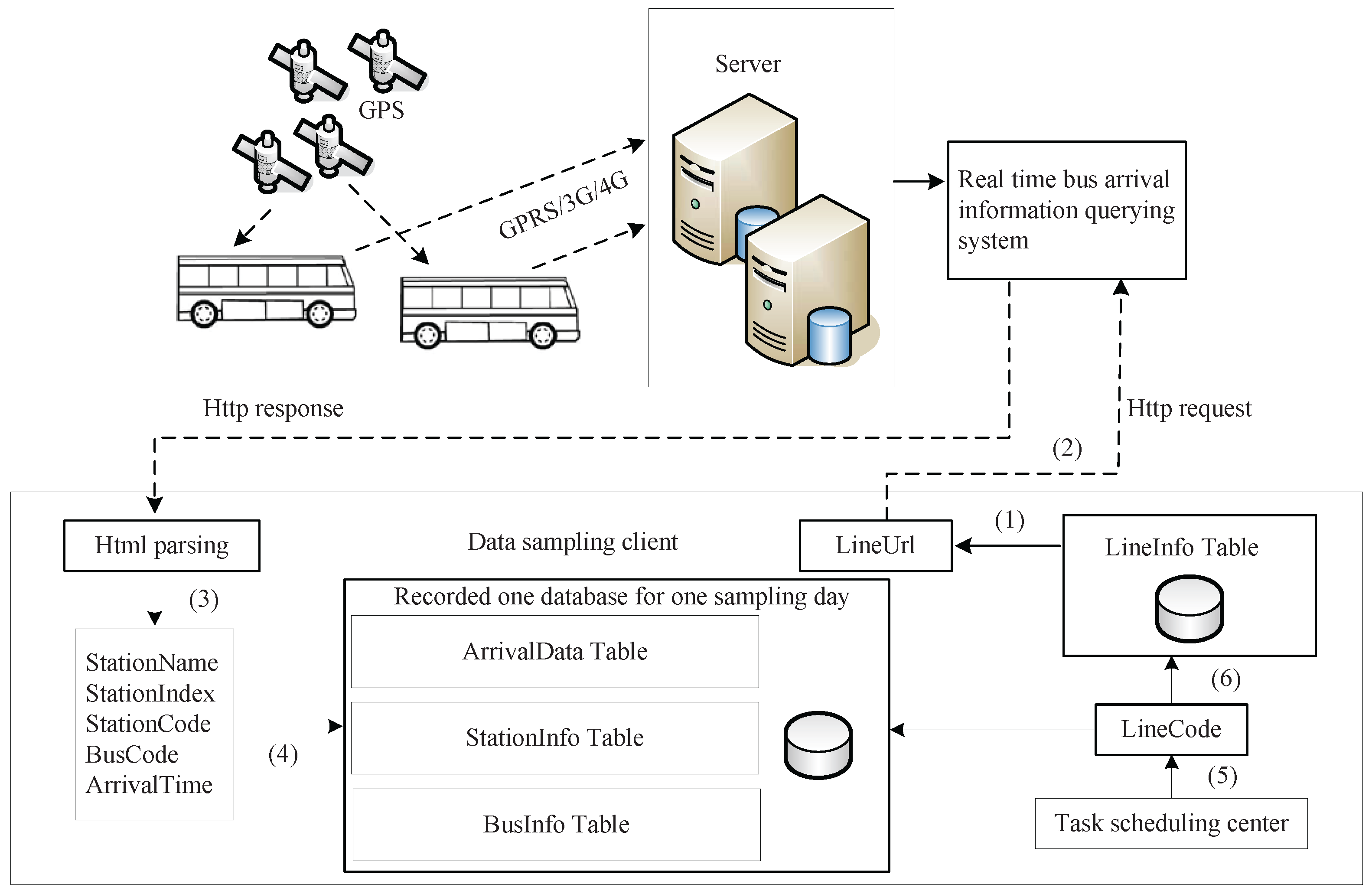
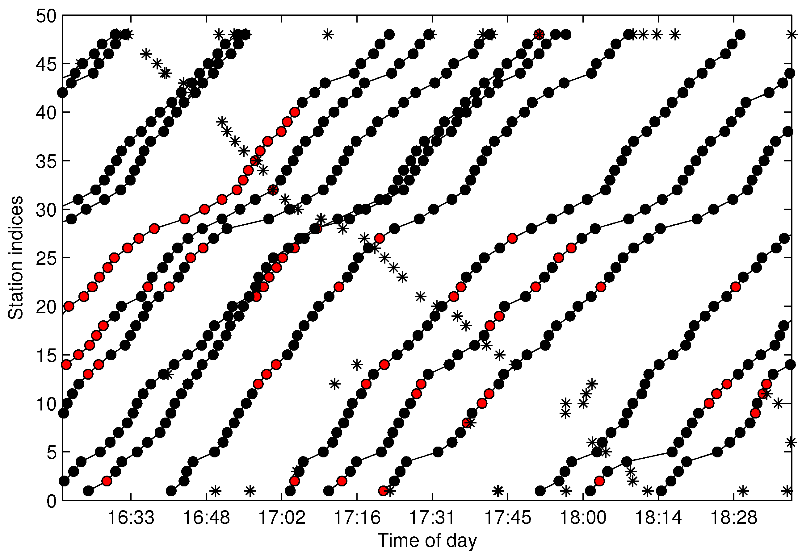
Data missing is very common in many real systems and can have a significant effect on the analysis of data. In our data acquisition project, almost all of the extracted trajectories are incomplete due to the arrival data missing randomly occurring along the stations. For the urban pubic transportation system, data missing may be caused by GPS positioning failure of the floating bus or networking problems when transmitting data. For data sampling, data missing will also happen in an unstable network. It is important that the missing data should be recovered firstly before mining the spatio-temporal properties of the trajectories.
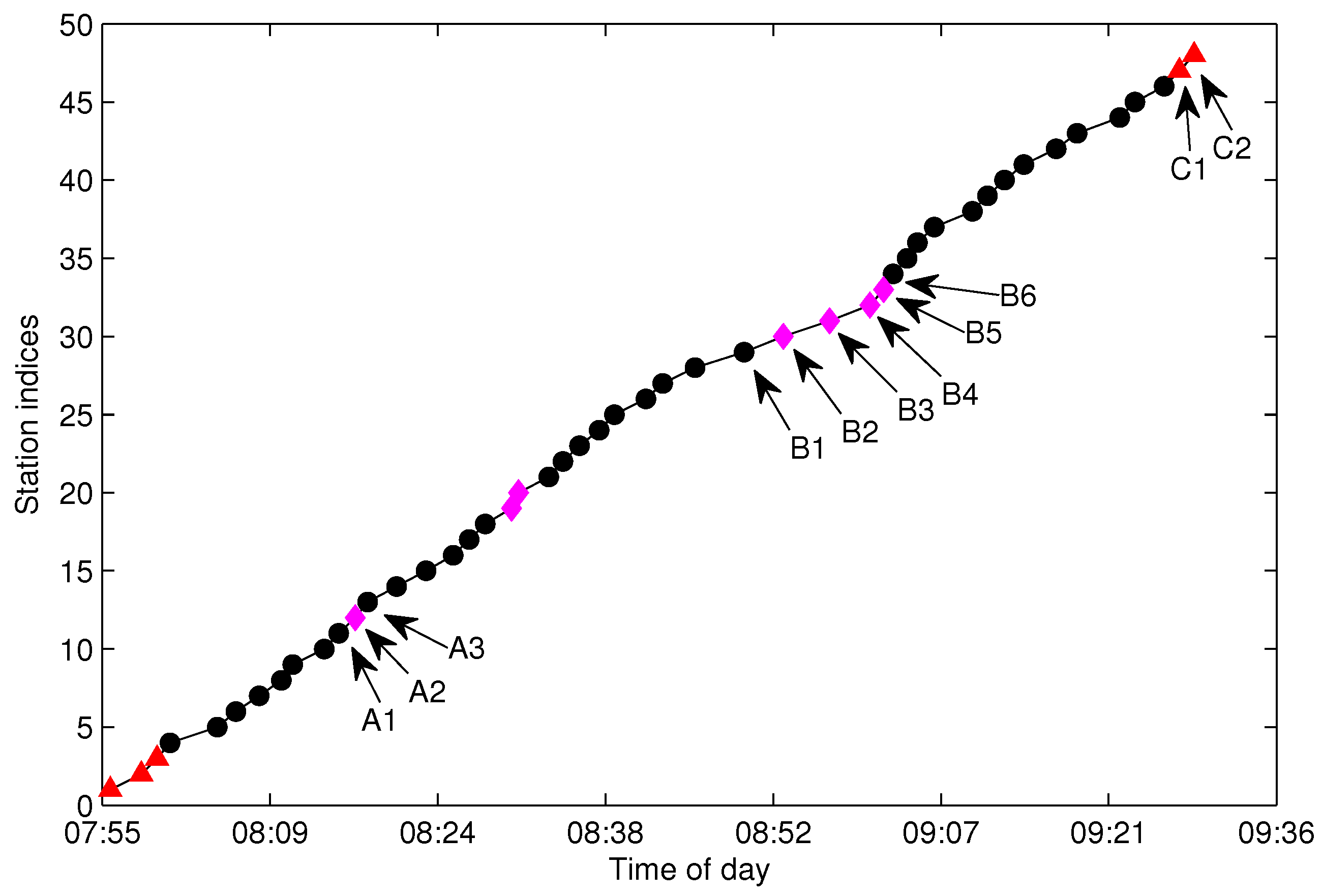
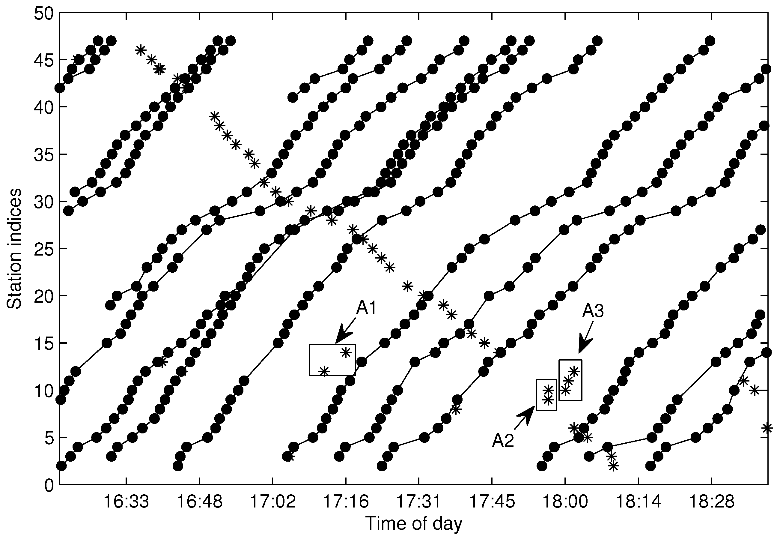
There are tens thousands of trajectories recorded in one day for the city of Suzhou with more than 500 bus lines. Time consumed algorithms for missing data recovery are not recommended for such a system. In this work, we propose two methods of data recovery corresponding to different types of missing data, both of which are easily implemented. The first one is contextual linear interpolation for missing data recovery (CLIMDR) for the cases of missing data inside the trajectory, as shown with the magenta dots in
Figure 9. The other one is median value interpolation for missing data recovery (MIMDR) for the cases of missing data outside the trajectory, as shown with the red dots in
Figure 9.
The CLIMDR method is context related and statistical. Taking the points
A1-A2-A3 shown in
Figure 9 as an example, the missing data of
A2 is recovered by:
where
is the arrival time of
Ai for
,
is the traveling time from
Ai to
Aj and
is the historical non-missing dataset selected from
by the station indices corresponding to
A1,
A2 and
A3. For data operation convenience,
(the one-route trajectories set of line
l) can be transformed into a two-dimensional data matrix
with
the arrival time at station
j of the
i-th trajectory.
is constructed from
by two steps:
set , where the first symbol “:” means selecting all rows of , and the second parameter set “” means selecting the corresponding columns of with the station index of ;
delete the rows of when any elements in the row equal zero (missing data).
The CLIMDR method is implemented based on the assumption that
and
are approximately linear with:
In Equation (
20), the parameters
and
are obtained with least square estimation from
as follows:
where
,
and
are constructed from
as follows:
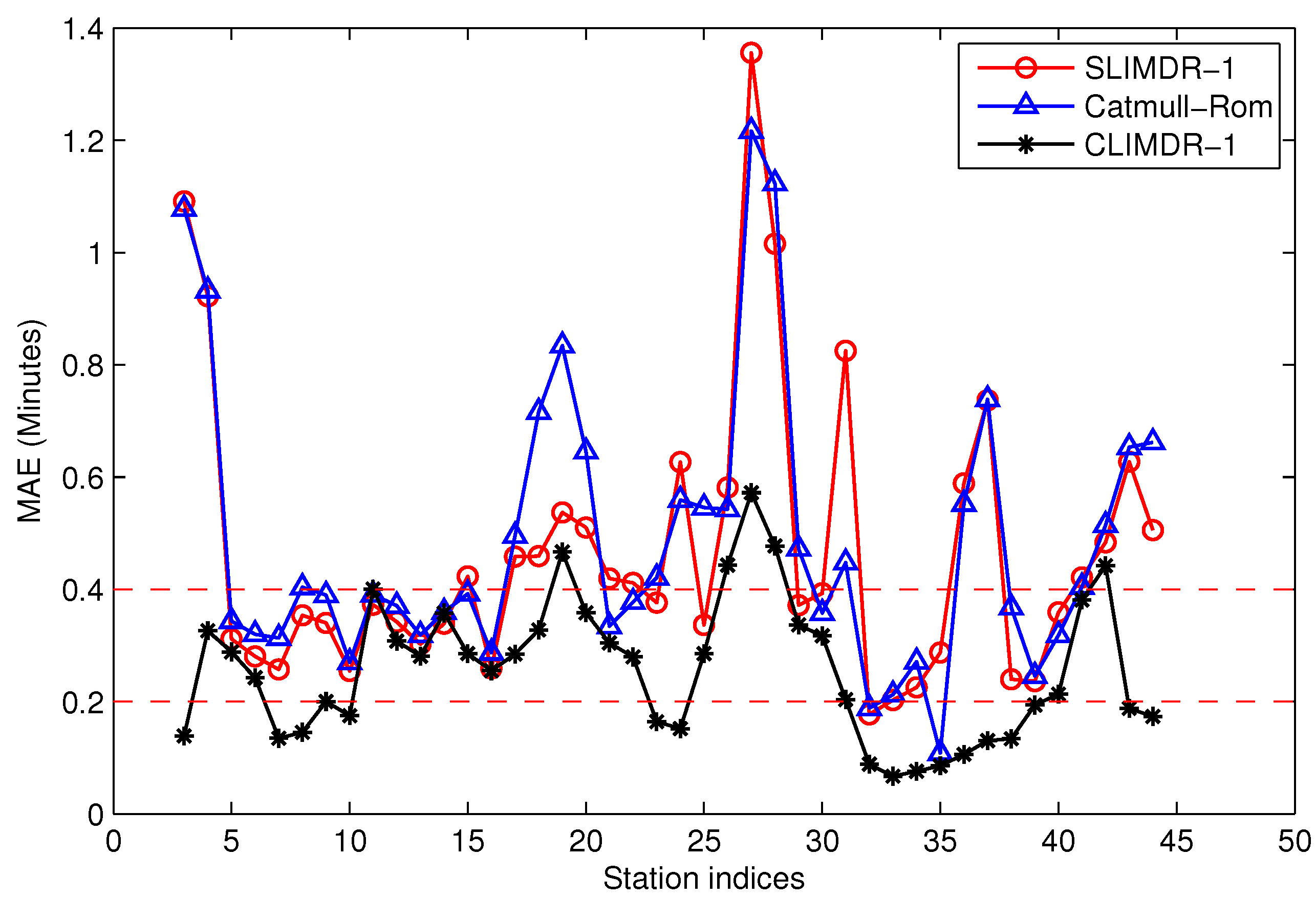
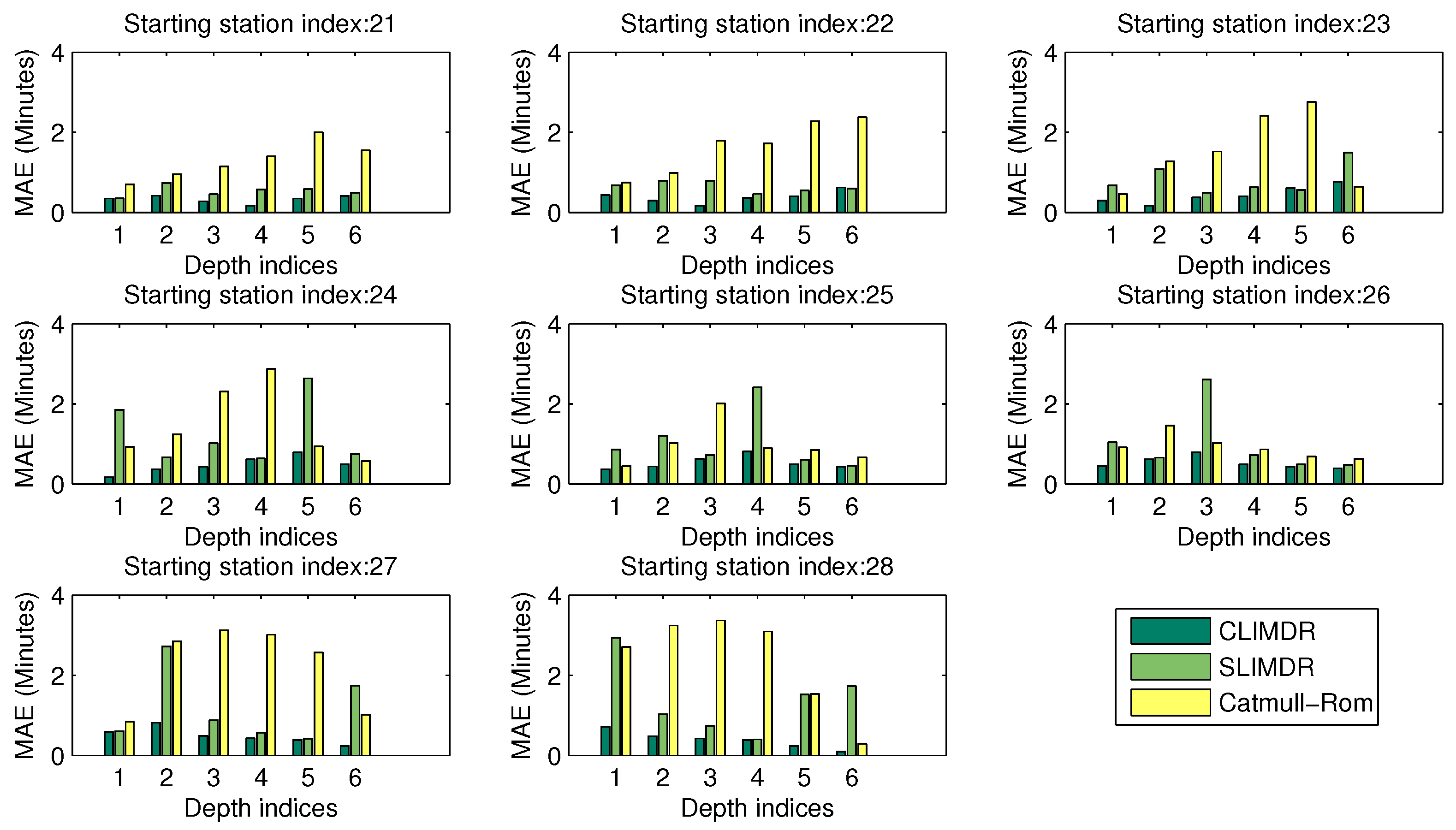
The CLIMDR method for the case of
A1-A2-A3 shown in
Figure 9 is called CLIMDR-1, which means recovering one depth missing datum, i.e., the number of successive missing data is one. Similarly, we call CLIMDR-
n for the
n-depth missing data recovery by the CLIMDR method. CLIMDR-
n is implemented by an iterative method. Taking the trajectory points
B1-B6 shown in
Figure 9 as an example, there are four missing data in
B1-B6; hence, the missing depth is four, and the corresponding recovery method is CLIMDR-4. In the interpolating procedure, we first recover
B2 by
and
; then,
B3 can be recovered by
and
. The interpolation procedure continues until
B5 is recovered.
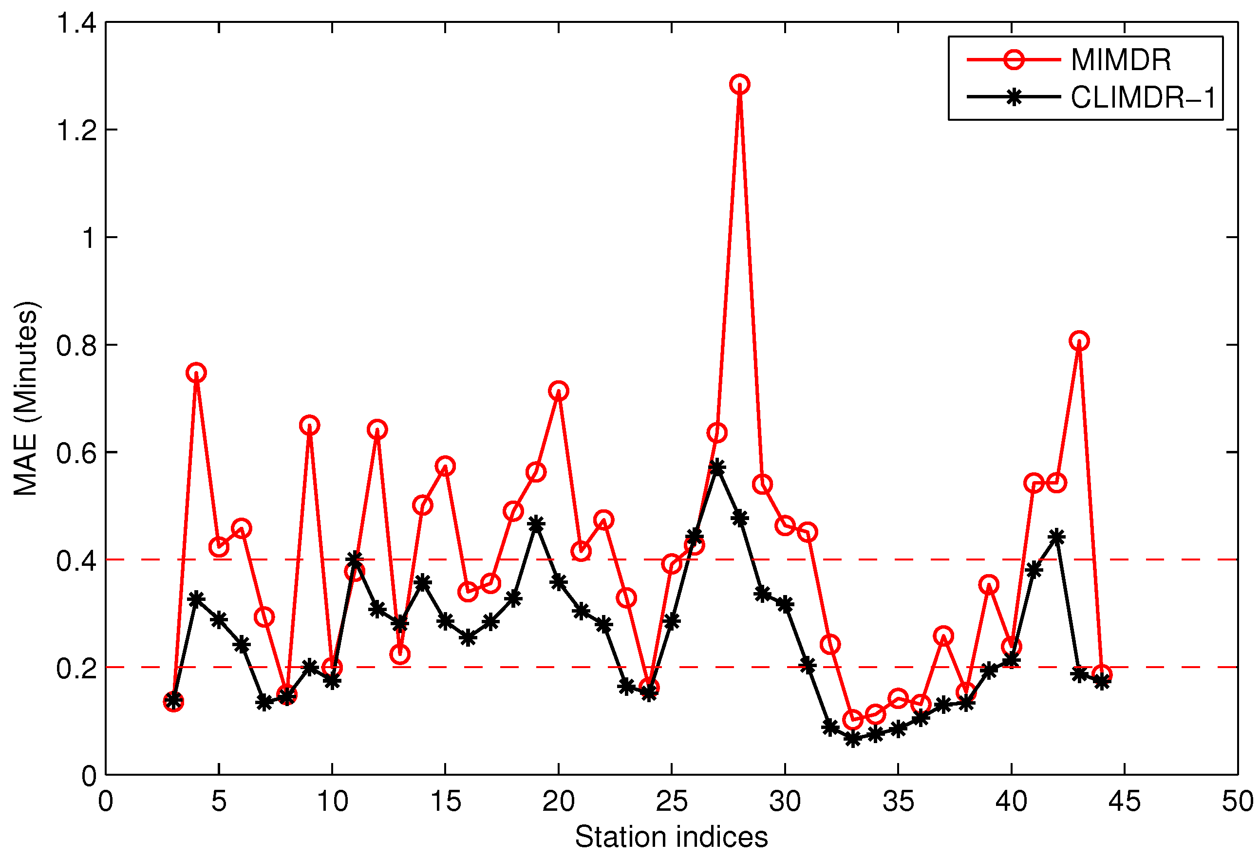
The MIMDR method is applied for the cases of missing data outside the extracted trajectory. In those cases, most of interpolation methods, including linear interpolation, kinematic interpolation [
23], Bezier curves [
24], Catmull-Rom curves [
25] and our proposed CLIMDR, are not available, since the head part or tail part of the data is also lost. In the MIMDR method, we firstly partition the data into the weekday set and weekend set. Then, we split the time of day into time slots with equal duration of 20 min and calculate the median value of traveling time in every time slot from the historical non-missing dataset. Finally, the missing data are recovered by the median value according to the time slot and weekday/weekend attributes. In practice, we only recover the starting and terminal stations of the trajectory by MIMDR to avoid accumulative errors. When the missing head or tail of the trajectory is recovered, the CLIMDR method can be applied again to recover the middle part of the trajectory.


