Model-Based Real-Time Non-Rigid Tracking


Abstract
1. Introduction
2. Related Works
2.1. Structure-From-Motion
2.2. Shape-From-Template
2.3. Non-Rigid Structure from Motion
2.4. Proposal
3. Algorithm Description
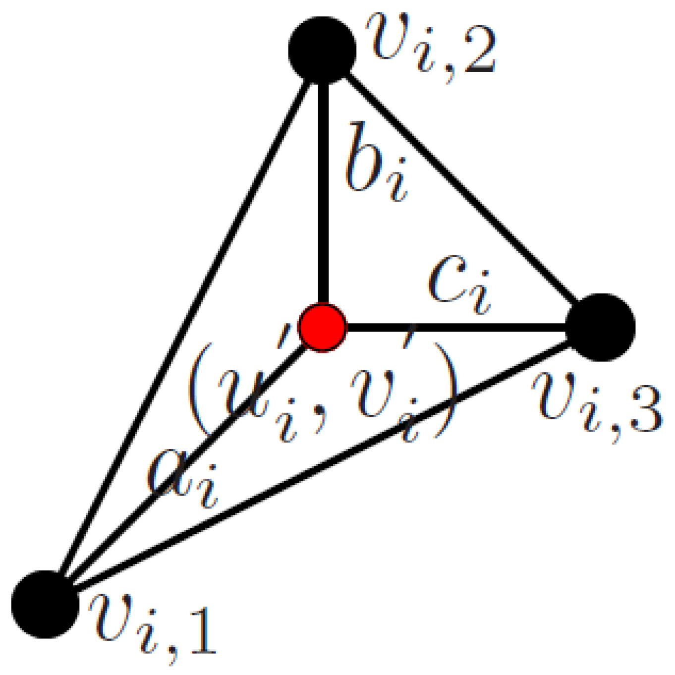
3.1. Measurement Model/Data Association
3.2. Feature Matching
3.2.1. PTAM-Based Matching Approach
- Affine warping described in [8] is kept to handle points whose local appearance is affected by a rigid motion.
- If the deformation causes significant changes in the appearance, affine warping is expected to fail. Then, we search features in a coarse-to-fine hierarchical correlation-based approach. To discard false positives, a married matching is applied in the lowest level of the pyramid in which the feature has been found. In case the correlation is too low or the distance is too high, the matching is considered not found. For a deeper explanation, we refer the readers to our publication in [52].
3.2.2. Descriptor-Based Matching Approach
3.3. Motion Modeling
3.4. EM Optimization
- Pose parameters (6 DoF): rotation R and translation T defined by the vector of parameters .
- Deformation parameters (K DoF): the set of K shape deformation coefficients L.
3.4.1. E-Step: Deformation Estimation
3.4.2. M-Step, Pose Estimation
3.5. Priors
4. Results
4.1. Performance Metrics
- 2D error:where F is the number of frames of the sequences, P is the number of points, are the re-projected features on the image and represent the image coordinates of the ground-truth points.
- 3D error:is the estimated shape and the ground truth shape.
4.2. Setup
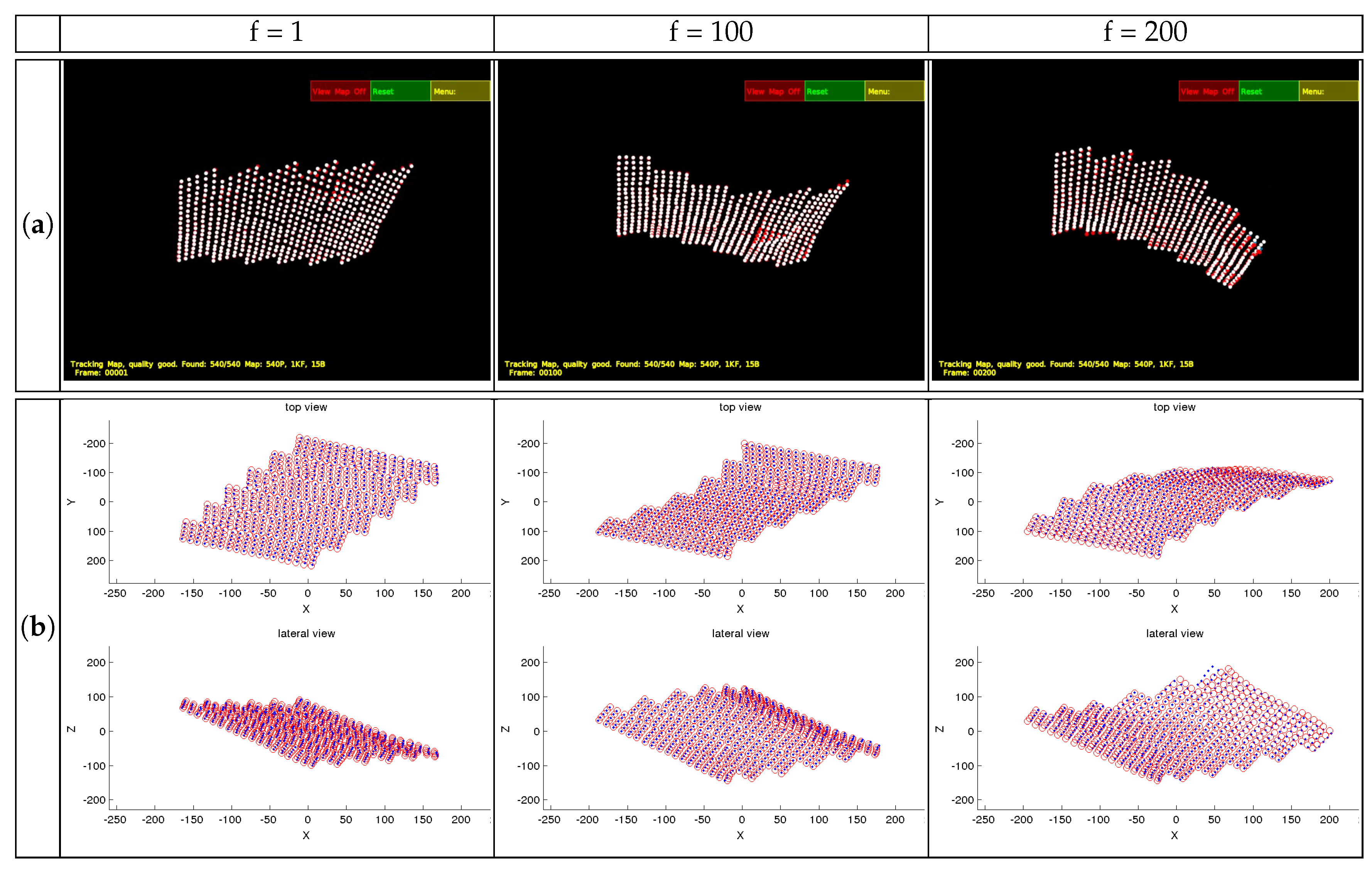
4.3. Flag Sequence
4.3.1. Performance Evaluation Based on Perfect Matching
4.3.2. Performance Evaluation Based on Visibility Degradation
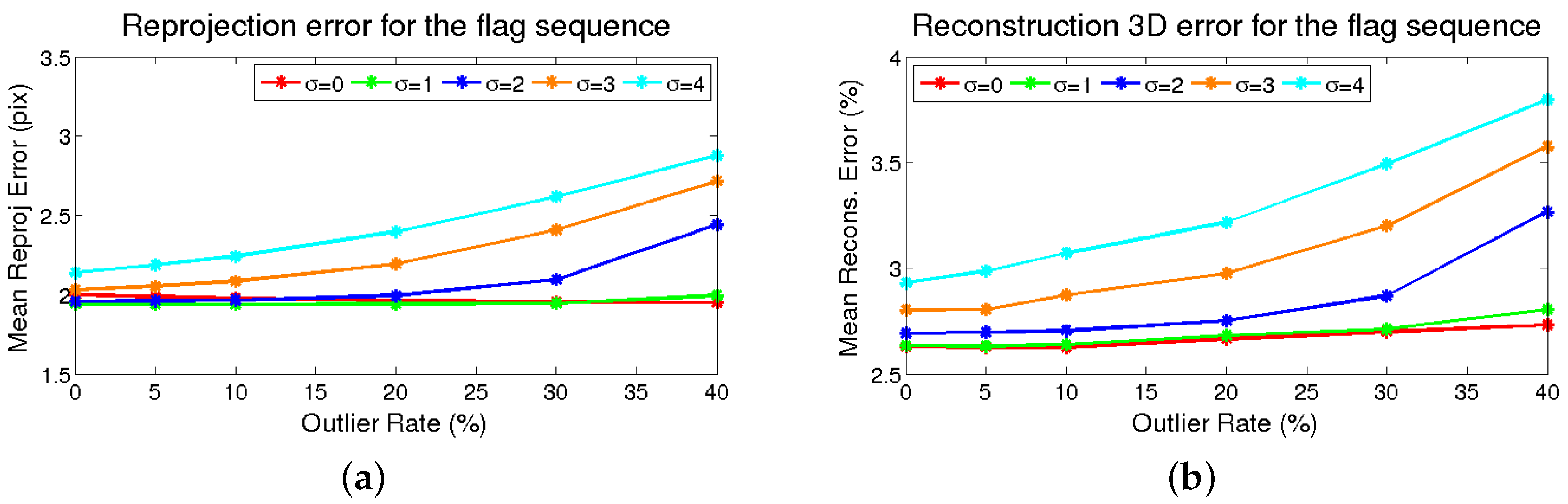
4.3.3. Performance Evaluation Based on Noise and Outliers
4.3.4. Performance Evaluation Based on the Number of Bases
4.3.5. Comparison with Other Methods of the State-Of-The-Art
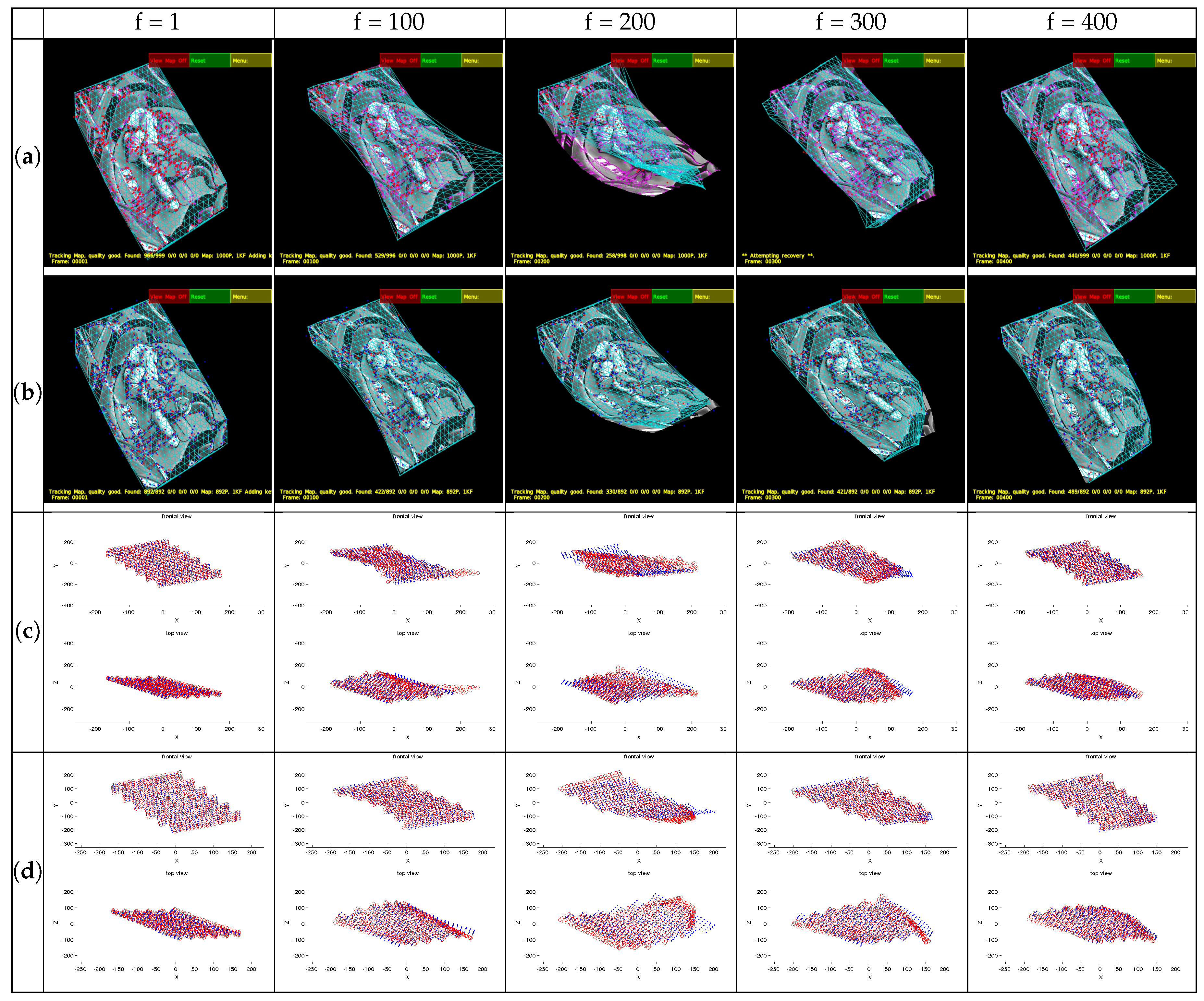
4.4. CMUfaceSequence
4.5. Point-Wise CVLab’s Kinect Paper
4.6. Rendered Flag Sequence
4.6.1. Evaluation of Visual Descriptors
4.6.2. Performance Evaluation Based on the Number of Bases
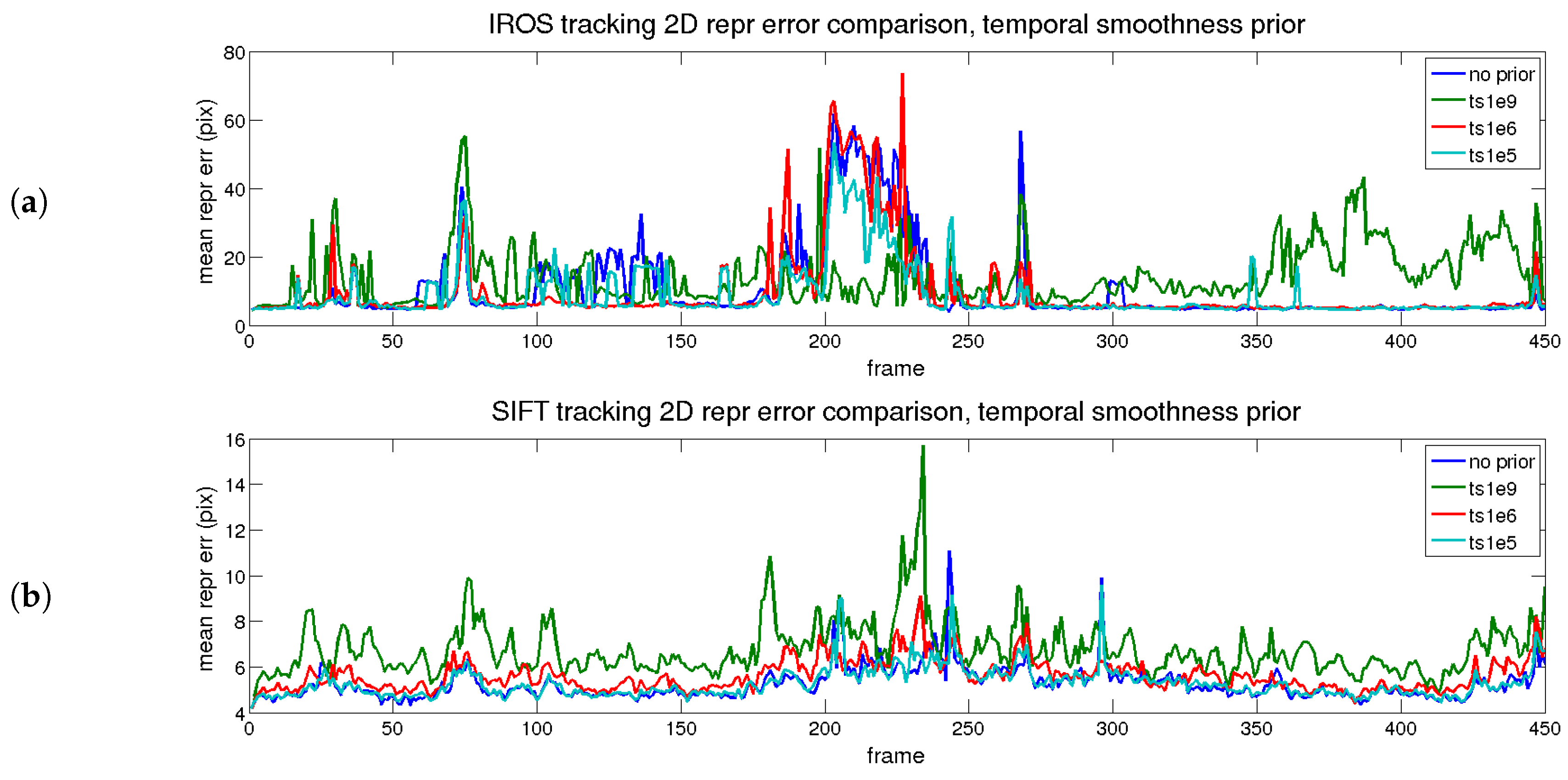
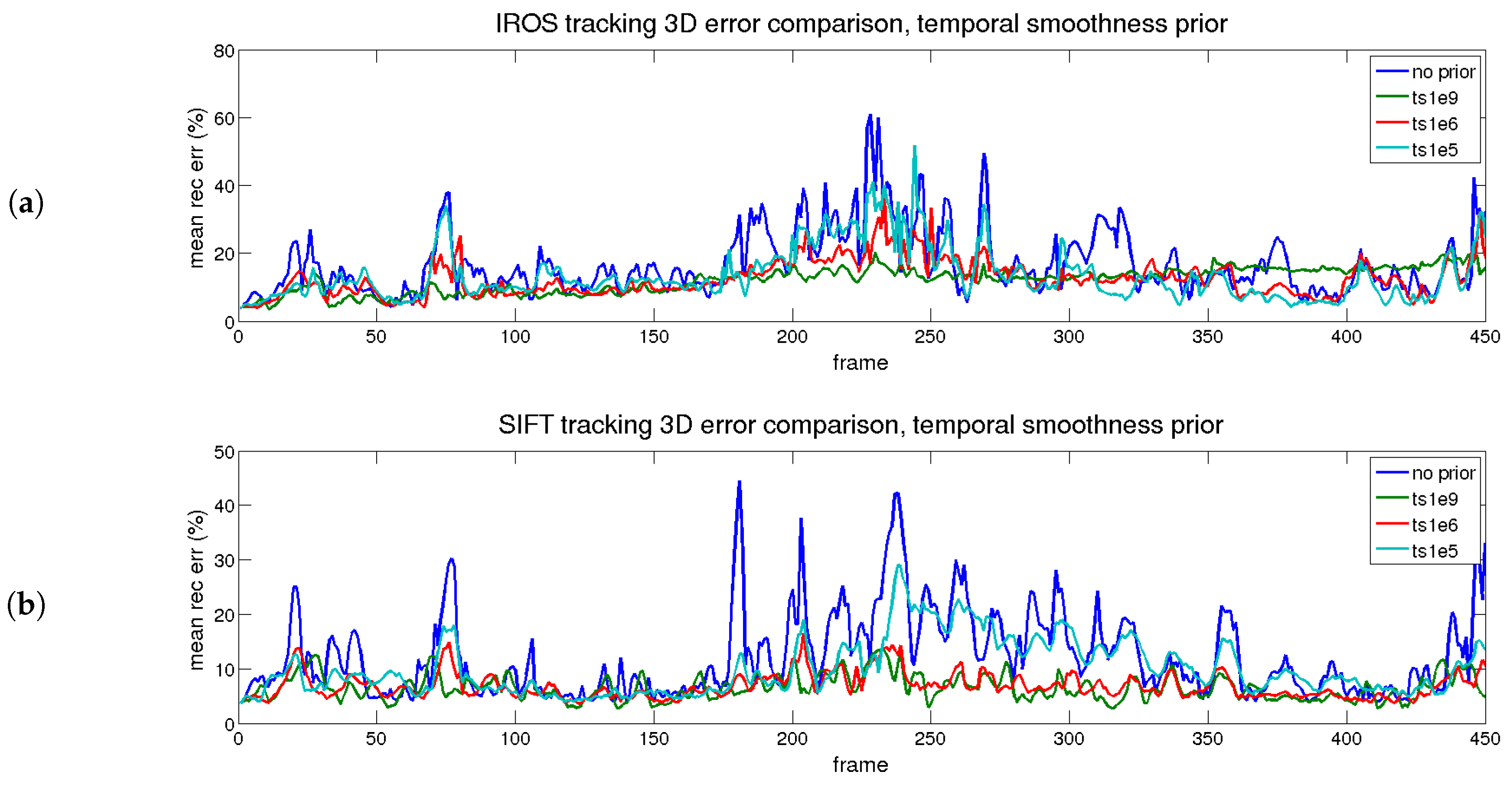
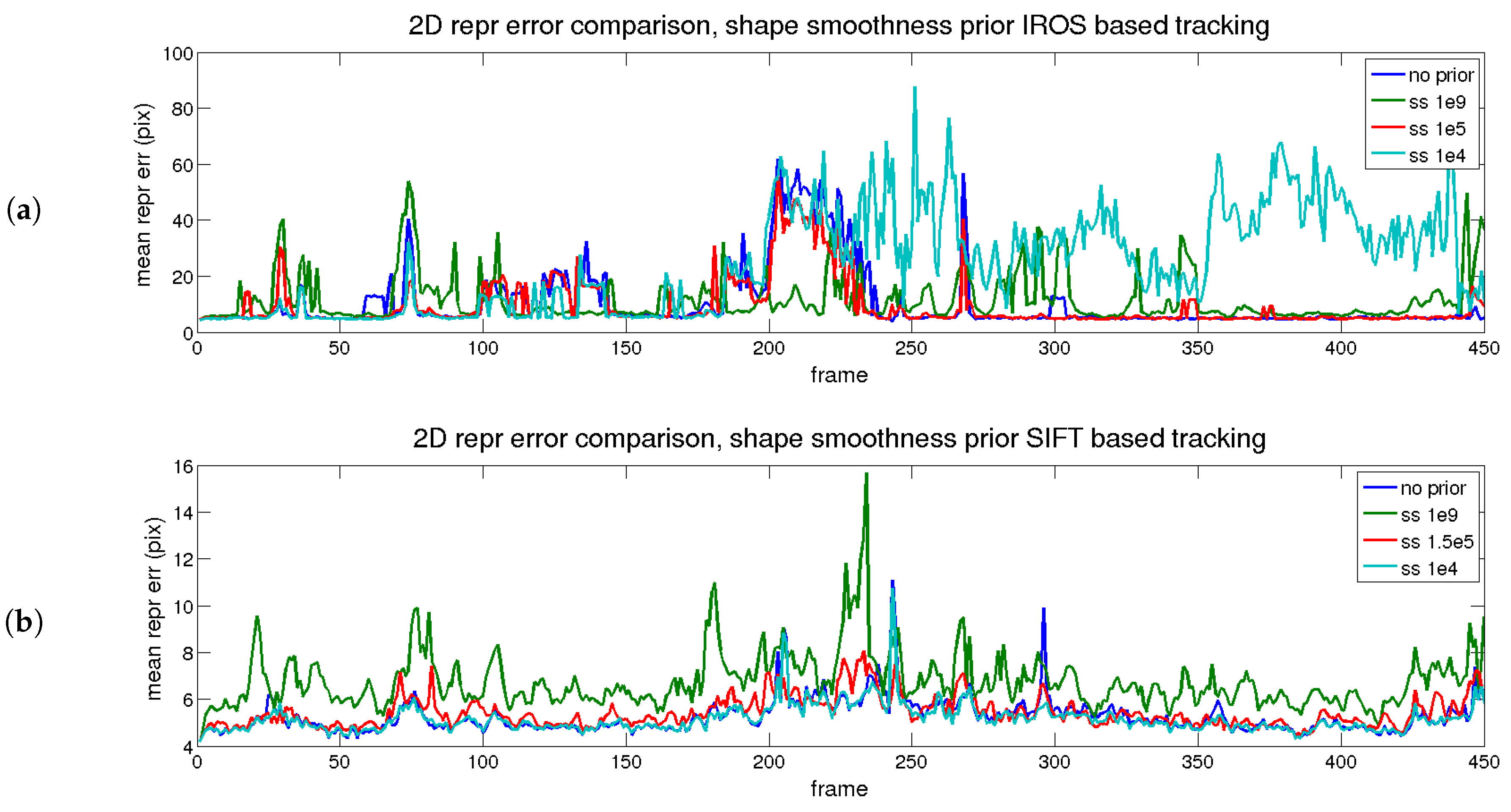
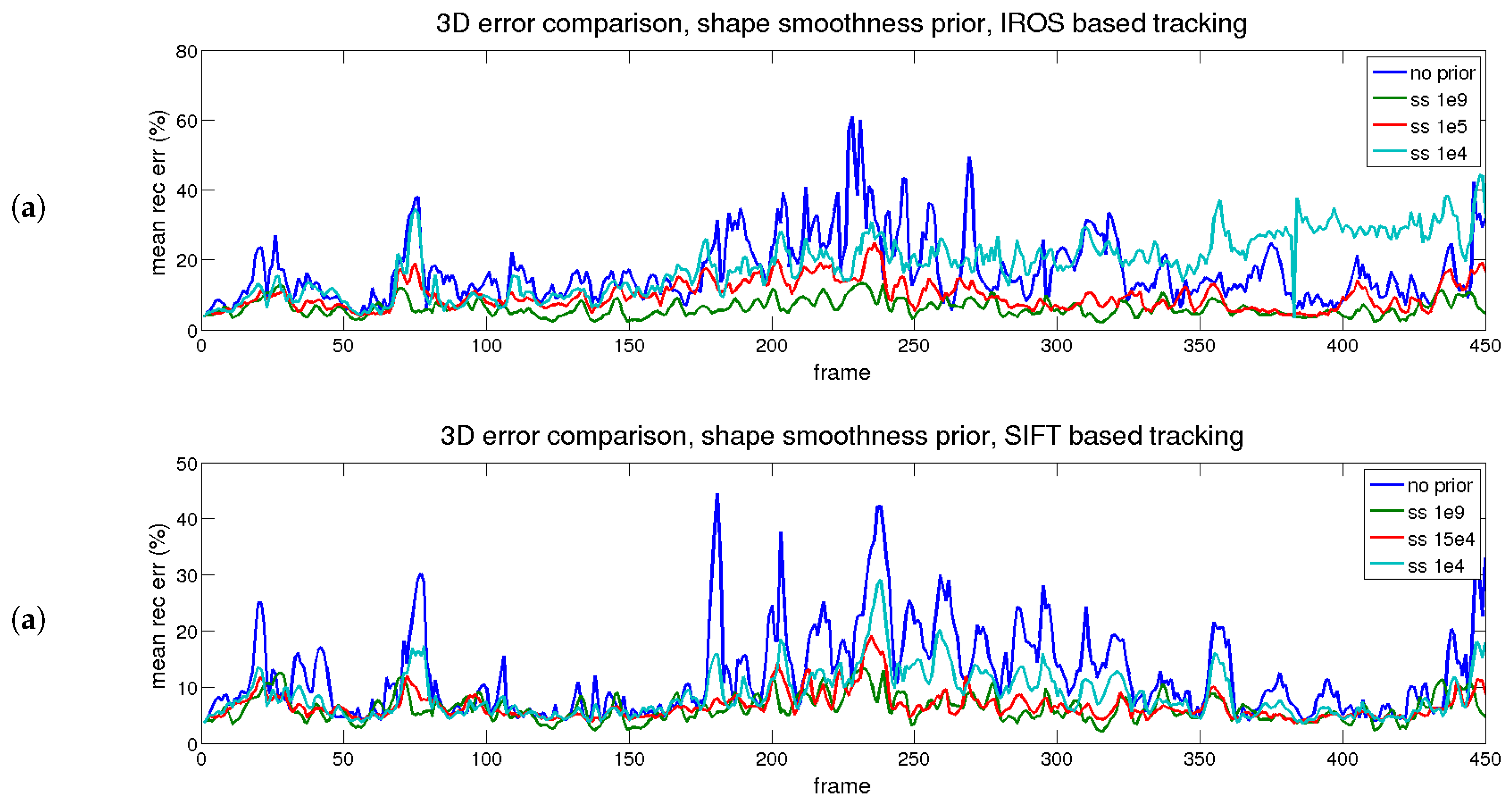
4.6.3. Performance Evaluation with Time and Shape Smoothing Priors
4.7. CVLab’s Kinect Paper
5. Conclusions
Acknowledgments
Author Contributions
Conflicts of Interest
References
- Hartley, R.I.; Zisserman, A. Multiple View Geometry in Computer Vision, 2nd ed.; Cambridge University Press: Cambridge, UK, 2004; ISBN 0521540518. [Google Scholar]
- Sturm, P.F.; Triggs, B. A Factorization Based Algorithm for Multi-Image Projective Structure and Motion. In Proceedings of the 4th European Conference on Computer Vision-Volume II—Volume II, ECCV ’96, Cambridge, UK, 15–18 April 1996; Springer-Verlag: London, UK, 1996; pp. 709–720. [Google Scholar]
- Dellaert, F.; Kaess, M. Square Root SAM: Simultaneous Localization and Mapping via Square Root Information Smoothing. Int. J. Robot. Res. 2006, 25, 1181–1203. [Google Scholar] [CrossRef]
- Davison, A.J.; Reid, I.D.; Molton, N.D.; Stasse, O. MonoSLAM: Real-time single camera SLAM. IEEE Trans. Pattern Anal. Mach. Intell. 2007, 29, 1052–1067. [Google Scholar] [CrossRef] [PubMed]
- Agarwal, S.; Snavely, N.; Simon, I.; Seitz, S.M.; Szeliski, R. Building Rome in a day. In Proceedings of the IEEE 12th International Conference on Computer Vision, ICCV 2009, Kyoto, Japan, 27 September–4 October 2009; pp. 72–79. [Google Scholar]
- Kyriakaki, G.; Doulamis, A.; Doulamis, N.; Ioannides, M.; Makantasis, K.; Protopapadakis, E.; Hadjiprocopis, A.; Wenzel, K.; Fritsch, D.; Klein, M.; et al. 4D Reconstruction of Tangible Cultural Heritage Objects from Web-Retrieved Images. Int. J. Herit. Digit. Era 2014, 3, 431–451. [Google Scholar] [CrossRef]
- Makantasis, K.; Doulamis, A.; Doulamis, N.; Ioannides, M. In the wild image retrieval and clustering for 3D cultural heritage landmarks reconstruction. Multimed. Tools Appl. 2016, 75, 3593–3629. [Google Scholar] [CrossRef]
- Klein, G.; Murray, D. Parallel Tracking and Mapping for Small AR Workspaces. In Proceedings of the 2007 6th IEEE and ACM International Symposium on Mixed and Augmented Reality, Nara, Japan, 13–16 November 2007; pp. 1–10. [Google Scholar]
- Newcombe, R.A.; Lovegrove, S.J.; Davison, A.J. DTAM: Dense Tracking and Mapping in Real-Time. In Proceedings of the 2011 IEEE International Conference on Computer Vision (ICCV), Barcelona, Spain, 6–13 November 2011; pp. 2320–2327. [Google Scholar]
- Bregler, C.; Hertzmann, A.; Biermann, H. Recovering Non-Rigid 3D Shape from Image Streams. In Proceedings of the IEEE Converence on Computer Vision and Pattern Recognition, Havana, Cuba, 9–12 September 2008; pp. 690–696. [Google Scholar]
- Torresani, L.; Hertzmann, A.; Bregler, C. Nonrigid Structure-from-motion: Estimating Shape and Motion with Hierarchical Priors. IEEE Trans. Pattern Anal. Mach. Intell. 2008, 30, 878–892. [Google Scholar] [CrossRef] [PubMed]
- Paladini, M.; Del Bue, A.; Stosic, M.; Dodig, M.; Xavier, J.; Agapito, L. Factorization for Non-Rigid and Articulated Structure Using Metric Projections. In Proceedings of the IEEE Conference on Computer Vision and Pattern Recognition, Miami, FL, USA, 20–25 June 2009; pp. 2898–2905. [Google Scholar]
- Del Bue, A.; Lladó, X.; Agapito, L. Non-Rigid Metric Shape and Motion Recovery from Uncalibrated Images Using Priors. In Proceedings of the 2006 IEEE Computer Society Conference on Computer Vision and Pattern Recognition (CVPR 2006), New York, NY, USA, 17–22 June 2006; pp. 1191–1198. [Google Scholar]
- Chhatkuli, A.; Pizarro, D.; Bartoli, A. Non-Rigid Shape-from-Motion for Isometric Surfaces using Infinitesimal Planarity. In Proceedings of the British Machine Vision Conference, BMVC 2014, Nottingham, UK, 1–5 September 2014. [Google Scholar]
- Parashar, S.; Pizarro, D.; Bartoli, A. Isometric Non-Rigid Shape-From-Motion in Linear Time. In Proceedings of the the IEEE Conference on Computer Vision and Pattern Recognition (CVPR), Las Vegas, NV, USA, 27–30 June 2016. [Google Scholar]
- Bartoli, A.; Collins, T. Template-Based Isometric Deformable 3D Reconstruction with Sampling-Based Focal Length Self-Calibration. In Proceedings of the IEEE Conference on Computer Vision and Pattern Recognition (CVPR), Portland, OR, USA, 23–28 June 2013. [Google Scholar]
- Bartoli, A.; Gérard, Y.; Chadebecq, F.; Collins, T.; Pizarro, D. Shape-from-template. IEEE Trans. Pattern Anal. Mach. Intell. 2015, 37, 2099–2118. [Google Scholar] [CrossRef] [PubMed]
- Fua, P.; Salzmann, M. Linear Local Models for Monocular Reconstruction of Deformable Surfaces. IEEE Trans. Pattern Anal. Mach. Intell. 2011, 33, 931–944. [Google Scholar]
- Ngo, D.T.; Östlund, J.; Fua, P. Template-Based Monocular 3D Shape Recovery Using Laplacian Meshes. IEEE Trans. Pattern Anal. Mach. Intell. 2016, 38, 172–187. [Google Scholar] [CrossRef] [PubMed]
- Gotardo, P.F.; Martinez, A.M. Non-Rigid Structure from Motion with Complementary Rank-3 Spaces. In Proceedings of the IEEE Conference on Computer Vision and Pattern Recognition, Washington, DC, USA, 20–25 June 2011; pp. 3065–3072. [Google Scholar]
- Paladini, M.; Bartoli, A.; Agapito, L. Sequential non-rigid structure-from-motion with the 3D-implicit low-rank shape model. In Proceedings of the 11th European Conference on Computer vision, Crete, Greece, 5–11 September 2010; pp. 15–28. [Google Scholar]
- Agudo, A.; Moreno-Noguer, F.; Calvo, B.; Montiel, J. Sequential Non-Rigid Structure from Motion using Physical Priors. IEEE Trans. Pattern Anal. Mach. Intell. 2016, 38, 979–994. [Google Scholar] [CrossRef] [PubMed]
- Agudo, A.; Calvo, B.; Montiel, J.M.M. Finite Element based Sequential Bayesian Non-Rigid Structure from Motion. In Proceedings of the Conference on Computer Vision and Pattern Recognition (CVPR), Providence, RI, USA, 16–21 June 2012; pp. 1418–1425. [Google Scholar]
- Agudo, A.; Montiel, J.M.M.; Agapito, L.; Calvo, B. Online Dense Non-Rigid 3D Shape and Camera Motion Recovery. In Proceedings of the British Machine Vision Conference, Nottingham, UK, 1–5 September 2014. [Google Scholar]
- Collins, T.; Pizarro, D.; Bartoli, A.; Canis, M.; Bourdel, N. Computer-Assisted Laparoscopic Myomectomy by Augmenting the Uterus with Pre-operative MRI Data. In Proceedings of the International Symposium on Mixed and Augmented Reality (ISMAR), Munich, Germany, 10–12 September 2014. [Google Scholar]
- Maier-Hein, L.; Groch, A.; Bartoli, A.; Bodenstedt, S.; Boissonnat, G.; Chang, P.L.; Clancy, N.; Elson, D.S.; Haase, S.; Heim, E.; et al. Comparative validation of single-shot optical techniques for laparoscopic 3-D surface reconstruction. IEEE Trans. Med. Imag. 2014, 33, 1913–1930. [Google Scholar] [CrossRef] [PubMed]
- Collins, T.; Bartoli, A. Realtime Shape-from-Template: System and Applications. In Proceedings of the 2015 IEEE International Symposium on Mixed and Augmented Reality, ISMAR 2015, Fukuoka, Japan, 29 September–3 October 2015; pp. 116–119. [Google Scholar]
- Newcombe, R.A.; Izadi, S.; Hilliges, O.; Molyneaux, D.; Kim, D.; Davison, A.J.; Pushmeet, K.; Shotton, J.; Hodges, S.; Fitzgibbon, A. KinectFusion: Real-Time Dense Surface Mapping and Tracking. In Proceedings of the 10th IEEE International Symposium on Mixed and Augmented Reality (ISMAR), Basel, Switzerland, 26–29 October 2011. [Google Scholar]
- Cootes, T.; Edwards, G.; Taylor, C. Active Appearance Models. In IEEE European Conference on Computer Vision; Springer: New York, NY, USA, 1998; pp. 484–498. [Google Scholar]
- Muñoz, E.; Buenaposada, J.M.; Baumela, L. A Direct Approach for Efficiently Tracking with 3D morphable models. In Proceedings of the International Conference on Computer Vision, Kyoto, Japan, 29 September–2 October 2009; pp. 1615–1622. [Google Scholar]
- Booth, J.; Roussos, A.; Zafeiriou, S.; Ponniah, A.; Dunaway, D. A 3D Morphable Model Learnt From 10,000 Faces. In Proceedings of the IEEE Conference on Computer Vision and Pattern Recognition (CVPR), Las Vegas, NV, USA, 27–30 June 2016. [Google Scholar]
- Zhou, Y.; Antonakos, E.; Alabort-i Medina, J.; Roussos, A.; Zafeiriou, S. Estimating Correspondences of Deformable Objects “In-The-Wild”. In Proceedings of the IEEE Conference on Computer Vision and Pattern Recognition (CVPR), Las Vegas, NV, USA, 27–30 June 2016. [Google Scholar]
- Brunet, F.; Hartley, R.; Bartoli, A.; Navab, N.; Malgouyres, R. Monocular Template-based Reconstruction of Smooth and Inextensible Surfaces. In Proceedings of the Tenth Asian Conference on Computer Vision (ACCV 2010), Queenstown, New Zealand, 8–12 November 2010; Volume 6494, pp. 52–66. [Google Scholar]
- Vicente, S.; Agapito, L. Soft Inextensibility Constraints for Template-Free Non-rigid Reconstruction. In Proceedings of the Computer Vision—ECCV 2012-12th European Conference on Computer Vision Part III, Florence, Italy, 7–13 October 2012; pp. 426–440. [Google Scholar]
- Pizarro, D.; Bartoli, A. Feature-Based Deformable Surface Detection with Self-Occlusion Reasoning. Int. J. Comput. Vis. 2012, 97, 54–70. [Google Scholar] [CrossRef]
- Sundaram, N.; Brox, T.; Keutzer, K. Dense point trajectories by GPU-accelerated large displacement optical flow. In European Conference on Computer Vision; Springer: Berlin, Germany, 2010; pp. 438–451. [Google Scholar]
- Chhatkuli, A.; Pizarro, D.; Collins, T.; Bartoli, A. Inextensible Non-Rigid Shape-from-Motion by Second-Order Cone Programming. In Proceedings of the 2016 IEEE Conference on Computer Vision and Pattern Recognition, CVPR 2016, Las Vegas, NV, USA, 27–30 June 2016; pp. 1719–1727. [Google Scholar]
- Agudo, A.; Calvo, B.; Montiel, J.M.M. 3D Reconstruction of Non-Rigid Surfaces in Real-Time Using Wedge Elements. In Proceedings of the Workshop on Non-Rigid Shape Analysis and Deformable Image Alignment (ECCVW), Firenze, Italy, 7 October 2012; pp. 113–122. [Google Scholar]
- Agudo, A.; Agapito, L.; Calvo, B.; Montiel, J.M.M. Good Vibrations: A Modal Analysis Approach for Sequential Non-Rigid Structure from Motion. In Proceedings of the Conference on Computer Vision and Pattern Recognition (CVPR), Columbus, OH, USA, 23–28 June 2014; pp. 1558–1565. [Google Scholar]
- Agudo, A.; Moreno-Noguer, F.; Calvo, B.; Montiel, J. Real-Time 3D Reconstruction of Non-Rigid Shapes with a Single Moving Camera. Comput. Vis. Image Underst. 2016, 153, 37–54. [Google Scholar] [CrossRef]
- Fayad, J.; Agapito, L.; Del Bue, A. Piecewise Quadratic Reconstruction of Non-Rigid Surfaces from Monocular Sequences. In Proceedings of the 11th European Conference on Computer Vision, Computer Vision—ECCV 2010, Part IV, Heraklion, Crete, Greece, 5–11 September 2010; pp. 297–310. [Google Scholar]
- Russell, C.; Fayad, J.; Agapito, L. Energy based multiple model fitting for non-rigid structure from motion. In Proceedings of the 24th IEEE Conference on Computer Vision and Pattern Recognition, CVPR 2011, Colorado Springs, CO, USA, 20–25 June 2011; pp. 3009–3016. [Google Scholar]
- Garg, R.; Roussos, A.; Agapito, L. Dense Variational Reconstruction of Non-rigid Surfaces from Monocular Video. In Proceedings of the IEEE Conference on Computer Vision and Pattern Recognition, Portland, OR, USA, 23–28 June 2013; pp. 1272–1279. [Google Scholar]
- Dai, Y.; Li, H.; He, M. A simple prior-free method for non-rigid structure-from-motion factorization. In Proceedings of the 2012 IEEE Conference on Computer Vision and Pattern Recognition, Providence, RI, USA, 16–21 June 2012; pp. 2018–2025. [Google Scholar]
- Akhter, I.; Sheikh, Y.; Khan, S.; Kanade, T. Nonrigid structure from motion in trajectory space. In Advances in Neural Information Processing Systems; MIT Press: Cambridge, MA, USA; London, UK, 2009; pp. 41–48. [Google Scholar]
- Russell, C.; Yu, R.; Agapito, L. Video Pop-up: Monocular 3D Reconstruction of Dynamic Scenes. In Computer Vision—ECCV 2014; Lecture Notes in Computer Science; Fleet, D., Pajdla, T., Schiele, B., Tuytelaars, T., Eds.; Springer: Berlin, Germany, 2014; Volume 8695, pp. 583–598. [Google Scholar]
- Newcombe, R.A.; Fox, D.; Seitz, S.M. DynamicFusion: Reconstruction and Tracking of Non-Rigid Scenes in Real-Time. In Proceedings of the IEEE Conference on Computer Vision and Pattern Recognition (CVPR), Boston, MA, USA, 7–12 June 2015. [Google Scholar]
- Hartley, R.I.; Vidal, R. Perspective Nonrigid Shape and Motion Recovery. In Proceedings of the 10th European Conference on Computer Vision, Computer Vision—ECCV 2008, Marseille, France, 12–18 October 2008; pp. 276–289. [Google Scholar]
- Bartoli, A.; Gay-Bellile, V.; Castellani, U.; Peyras, J.; Olsen, S.I.; Sayd, P. Coarse-to-fine low-rank structure-from-motion. In Proceedings of the 2008 IEEE Computer Society Conference on Computer Vision and Pattern Recognition (CVPR 2008), Anchorage, AK, USA, 24–26 June 2008. [Google Scholar]
- Yu, R.; Russell, C.; Campbell, N.D.F.; Agapito, L. Direct, Dense, and Deformable: Template-Based Non-Rigid 3D Reconstruction From RGB Video. In Proceedings of the IEEE International Conference on Computer Vision (ICCV), Santiago, Chile, 7–13 December 2015. [Google Scholar]
- Klein, G.; Murray, D. Parallel Tracking and Mapping on a Camera Phone. In Proceedings of the Eigth IEEE and ACM International Symposium on Mixed and Augmented Reality (ISMAR’09), Orlando, FL, USA, 19–22 October 2009. [Google Scholar]
- Bronte, S.; Paladini, M.; Bergasa, L.M.; Agapito, L.; Arroyo, R. Real-time sequential model-based non-rigid SFM. In Proceedings of the 2014 IEEE/RSJ International Conference on Intelligent Robots and Systems, Chicago, IL, USA, 14–18 September 2014; pp. 1026–1031. [Google Scholar]
- Moreno-Noguer, F.; Porta, J.M. Probabilistic Simultaneous Pose and Non-Rigid Shape Recovery. In Proceedings of the IEEE Conference on Computer Vision and Pattern Recognition, Colorado Springs, CO, USA, 20–25 June 2011; pp. 1289–1296. [Google Scholar]
- Rosten, E.; Drummond, T. Machine learning for high-speed corner detection. In European Conference on Computer Vision; Springer: Berlin, Germany, 2006; Volume 1, pp. 430–443. [Google Scholar]
- Itseez. Open Source Computer Vision Library, 2015. Available online: https://github.com/itseez/opencv (accessed on 30 September 2017).
- Alcantarilla, P.F.; Bartoli, A.; Davison, A.J. KAZE features. In European Conference on Computer Vision; Springer: Berlin, Germany, 2012; pp. 214–227. [Google Scholar]
- Alcantarilla, P.F.; Nuevo, J.; Bartoli, A. Fast Explicit Diffusion for Accelerated Features in Nonlinear Scale Spaces. In Proceedings of the British Machine Vision Conference (BMVC), Bristol, UK, 9–13 September 2013. [Google Scholar]
- Rublee, E.; Rabaud, V.; Konolige, K.; Bradski, G. ORB: An efficient alternative to SIFT or SURF. In Proceedings of the 2011 International Conference on Computer Vision, Barcelona, Spain, 6–13 November 2011; pp. 2564–2571. [Google Scholar]
- Leutenegger, S.; Chli, M.; Siegwart, R.Y. BRISK: Binary robust invariant scalable keypoints. In Proceedings of the 2011 International Conference on Computer vision, Barcelona, Spain, 6–13 November 2011; pp. 2548–2555. [Google Scholar]
- Lowe, D.G. Distinctive image features from scale-invariant keypoints. Int. J. Comput. Vis. 2004, 60, 91–110. [Google Scholar] [CrossRef]
- Bay, H.; Tuytelaars, T.; Van Gool, L. Surf: Speeded up robust features. In European Conference on Computer Vision; Springer: Berlin, Germany, 2006; pp. 404–417. [Google Scholar]
- Joseph Tan, D.; Holzer, S.; Navab, N.; Ilic, S. Deformable Template Tracking in 1 ms. In Proceedings of the British Machine Vision Conference, Nottingham, UK, 1–5 September 2014. [Google Scholar]
- Simo-Sierra, E.; Torras, C.; Moreno-Noger, F. DaLI: Deformation and Light Invariant Descriptor. Int. J. Comput. Vis. 2015, 115, 136–154. [Google Scholar] [CrossRef]
- Benhimane, S.; Malis, E. Homography-based 2D Visual Tracking and Servoing. Int. J. Robot. Res. 2007, 26, 661–676. [Google Scholar] [CrossRef]
- Torresani, L.; Hertzmann, A.; Bregler, C. Learning Non-Rigid 3D Shape from 2D Motion. In Advances in Neural Information Processing Systems 16; MIT Press: Cambridge, MA, USA, 2003; pp. 1555–1562. [Google Scholar]
- Dellaert, F. The Expectation Maximization Algorithm; Technical Report; Georgia Institute of Technology, College of Computing: Atlanta, Georgia, 2002. [Google Scholar]
- Tukey, J.W. A survey of sampling from contaminated distributions. Contrib. Probab. Stat. 1960, 2, 448–485. [Google Scholar]
- Gower, J.C.; Dijksterhuis, G.B. Procrustes Problems; Oxford Statistical Science Series; Oxford University Press: New York, NY, USA, 2004. [Google Scholar]
- Lee, M.; Cho, J.; Oh, S. Consensus of Non-Rigid Reconstructions. In Proceedings of the IEEE Conference on Computer Vision and Pattern Recognition (CVPR), Las Vegas, NV, USA, 27–30 June 2016. [Google Scholar]
- Varol, A.; Shaji, A.; Salzmann, M.; Fua, P. Monocular 3D Reconstruction of Locally Textured Surfaces. IEEE Trans. Pattern Anal. Mach. Intell. 2012, 34, 1118–1130. [Google Scholar] [CrossRef] [PubMed]
- Garg, R.; Roussos, A.; de Agapito, L. Robust Trajectory-Space TV-L1 Optical Flow for Non-rigid Sequences. In Proceedings of the Energy Minimization Methods in Computer Vision and Pattern Recognition, Saint Petersburg, Russia, 25–27 July 2011; Volume 6819, pp. 300–314. [Google Scholar]
- Varol, A.; Salzmann, M.; Fua, P.; Urtasun, R. A constrained latent variable model. In Proceedings of the IEEE Computer Society, Conference on Computer Vision and Pattern Recognition, Providence, RI, USA, 16–21 June 2012; pp. 2248–2255. [Google Scholar]
- Chhatkuli, A.; Pizarro, D.; Bartoli, A. Stable Template-Based Isometric 3D Reconstruction in All Imaging Conditions by Linear Least-Squares. In Proceedings of the 2014 IEEE Conference on Computer Vision and Pattern Recognition, CVPR 2014, Columbus, OH, USA, 23–28 June 2014; pp. 708–715. [Google Scholar]
- Salzmann, M. Continuous Inference in Graphical Models with Polynomial Energies. In Proceedings of the IEEE Computer Society, Computer Vision and Pattern Recognition (CVPR), Portland, OR, USA, 23–28 June 2013; pp. 1744–1751. [Google Scholar]


| #Bases (K) | 2D Error (pix) | 3D Error (%) |
|---|---|---|
| 5 | 4.56 | 3.84 |
| 7 | 3.62 | 3.21 |
| 15 | 2 | 2.63 |
| 25 | 1.34 | 2.1 |
| 30 | 1.18 | 1.93 |
| Method | 2D Error (px) | 3D Error (%) | Rank | Tproc (fps) | Model | ProcType | Impl. |
|---|---|---|---|---|---|---|---|
| [21] | 6.14 | 91.65 | 7 (max) | 20 min (0.37) | auto | seq. | MATLAB |
| [20] | 29.79 | 66.65/16.09 1 | 5 | 36 min (0.21) | auto | batch | MATLAB |
| [11] | 11.65 | 15.59/13.25 1 | 4 | 10 h (0.01) | auto | batch | MATLAB |
| [12] | 1.9 | 29.724/17.61 1 | 9 | 19 seg(23.68) | auto | batch | MATLAB |
| [34] | - | 1.79 | - | - | auto | batch | MATLAB |
| [42] | - | 1.29/3.25 1 | - | - | auto | batch | MATLAB |
| [69] | ~2 | n.a./3.8 | - | >>28 h | auto | batch | MATLAB |
| [44] | - | n.a./17.41 1 | - | >>16 h | auto | batch | MATLAB |
| [24] | - | 3.28 (K = 10) 2.81 (K = 40) | 10–40 | 708 seg (K = 10) (0.64) 1045.5 seg (K = 40) (0.43) | auto | seq. | MATLAB |
| Our approach | 2 | 2.63 | 15 | 5 seg. (90) | priory | seq. | C++ |
| Method | 2D Error (px) | 3D Error (%) | Rank | Tproc (fps) | Model | Proc Type | Impl. |
|---|---|---|---|---|---|---|---|
| [21] | 1.06 | 3.18 | 8 (max) | 14 min (0.37) | auto | seq. | MATLAB |
| [20] | 0.6 | 3.19 | 5 | 43 seg. (7.35) | auto | batch | MATLAB |
| [11] | 6.42/32.39 | 9.9/56.06 | 5/15 | 78/606 seg. (4.05/0.52) | auto | batch | MATLAB |
| [12] | 1.06 | 2.43 | 12 | 13 seg (24.3) | auto | batch | MATLAB |
| Our approach | 0.26 | 1.01 | 15 | 4.5 seg. (69.78) | priory | seq. | C++ |
| Descriptor | Matcher | 2D Error (px) | 3D Error (%) | tp (s/fps) | Map Pts |
|---|---|---|---|---|---|
| PTAM | PTAM | 40.12 | 104.54 | 102/4.4 | 350 |
| IROS | PTAM-like | 9.51 | 16.65 | 26/17.3 | 972 |
| AKAZE | Brute force | 5.68 | 12.42 | 27/16.6 | 607 |
| BRISK | Brute force | 5.98 | 14.27 | 56/8 | 1000 |
| ORB | Brute force | 5.67 | 12.71 | 29/15.5 | 1000 |
| KAZE | Brute force | 5.55 | 13.12 | 49/9.2 | 347 |
| SIFT | Brute force | 5.27 | 12.04 | 87/5.2 | 892 |
| SURF | Brute force | 5.4 | 14.11 | 29/15.5 | 650 |
| Matching | #Bases | 2D Error (pix) | 3D Error (%) |
|---|---|---|---|
| IROS | 7 | 8.83 | 9.19 |
| IROS | 15 | 9.51 | 16.65 |
| IROS | 30 | 13.2 | 34.23 |
| SIFT | 7 | 5.76 | 6.53 |
| SIFT | 15 | 5.27 | 12.04 |
| SIFT | 30 | 5.23 | 17.91 |
| Desc. | Prior Type | Value | 2D Error (px) | 3D Error (%) |
|---|---|---|---|---|
| PTAM | none | 0 | 40.12 | 104.54 |
| Point-wise ideal Matching | none | 0 | 2 | 2.63 |
| IROS | none | 0 | 9.51 | 16.65 |
| IROS | time | 1e5 | 8.92 | 13.38 |
| IROS | time | 1e6 | 9.76 | 12.42 |
| IROS | time | 1e9 | 14.37 | 12.04 |
| IROS | shape | 1e4 | 24.05 | 18.31 |
| IROS | shape | 1e5 | 9.38 | 9.54 |
| IROS | shape | 1e9 | 11.62 | 6.2 |
| IROS | both | 1e5/1e5 | 8.72 | 8.95 |
| SIFT | none | 0 | 5.27 | 12.04 |
| SIFT | time | 1e5 | 5.29 | 9.93 |
| SIFT | time | 1e6 | 5.64 | 6.79 |
| SIFT | time | 1e9 | 6.79 | 6.51 |
| SIFT | shape | 1e4 | 5.18 | 8.48 |
| SIFT | shape | 1.5e5 | 5.45 | 6.56 |
| SIFT | shape | 1e9 | 6.80 | 6.2 |
| SIFT | both | 1e5/1.5e5 | 5.48 | 6.46 |
| Desc. | Prior Type | Value | #Bases | 2D Error (px) | Depth Error (mm) |
|---|---|---|---|---|---|
| Point-wise ideal Matching | none | 0 | 15 | 9.06 | 10.39 |
| Point-wise ideal Matching | none | 0 | 50 | 7.98 | 10.35 |
| IROS | none | 0 | 15 | 26.28 | 10.34 |
| IROS | time | 1e3 | 15 | 26.45 | 14.34 |
| IROS | shape | 1e4 | 15 | 27.48 | 10.38 |
| IROS | none | 0 | 50 | 24.77 | 11.44 |
| IROS | time | 1e3 | 50 | 24.82 | 11.37 |
| IROS | shape | 1e4 | 50 | 24.35 | 10.68 |
| SIFT | none | 0 | 15 | 23.34 | 10.63 |
| SIFT | time | 1e3 | 15 | 23.36 | 10.60 |
| SIFT | shape | 1e4 | 15 | 23.43 | 10.48 |
| SIFT | none | 0 | 50 | 24.47 | 13.64 |
| SIFT | time | 1e3 | 50 | 24.45 | 13.67 |
| SIFT | shape | 1e4 | 50 | 23.62 | 11.17 |
| Method | Depth Error (mm) | Rank | Tproc (fps) | Model | Proc Type |
|---|---|---|---|---|---|
| [72] | 7.23 | - | - | priory | batch |
| [72] (PCA) | 11.68 | - | - | priory | batch |
| [73] | 6.9 | - | - | priory | sequential |
| [74] | 5.57 | - | 959 (0.2) | priory | sequential |
| Our approach (SIFT) | 13.65 | 50 | 90 (2) | priory | sequential |
| Our approach (IROS) | 11.44 | 50 | 17 (11.24) | priory | sequential |
© 2017 by the authors. Licensee MDPI, Basel, Switzerland. This article is an open access article distributed under the terms and conditions of the Creative Commons Attribution (CC BY) license (http://creativecommons.org/licenses/by/4.0/).
Share and Cite
Bronte, S.; Bergasa, L.M.; Pizarro, D.; Barea, R. Model-Based Real-Time Non-Rigid Tracking. Sensors 2017, 17, 2342. https://doi.org/10.3390/s17102342
Bronte S, Bergasa LM, Pizarro D, Barea R. Model-Based Real-Time Non-Rigid Tracking. Sensors. 2017; 17(10):2342. https://doi.org/10.3390/s17102342
Chicago/Turabian StyleBronte, Sebastián, Luis M. Bergasa, Daniel Pizarro, and Rafael Barea. 2017. "Model-Based Real-Time Non-Rigid Tracking" Sensors 17, no. 10: 2342. https://doi.org/10.3390/s17102342
APA StyleBronte, S., Bergasa, L. M., Pizarro, D., & Barea, R. (2017). Model-Based Real-Time Non-Rigid Tracking. Sensors, 17(10), 2342. https://doi.org/10.3390/s17102342