
Research on the Lift-off Effect of Receiving Longitudinal Mode Guided Waves in Pipes Based on the Villari Effect


Abstract
:1. Introduction
2. Theory Background
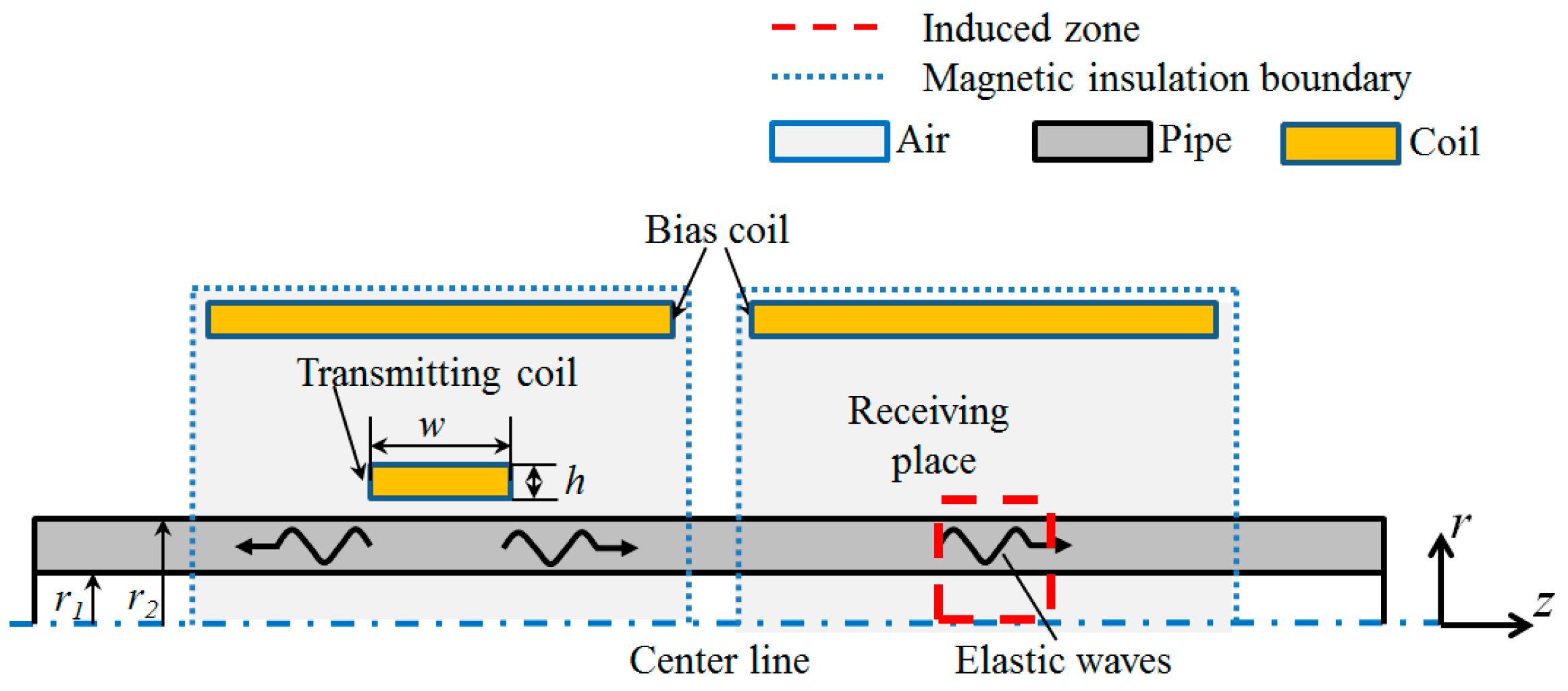
3. FE Model
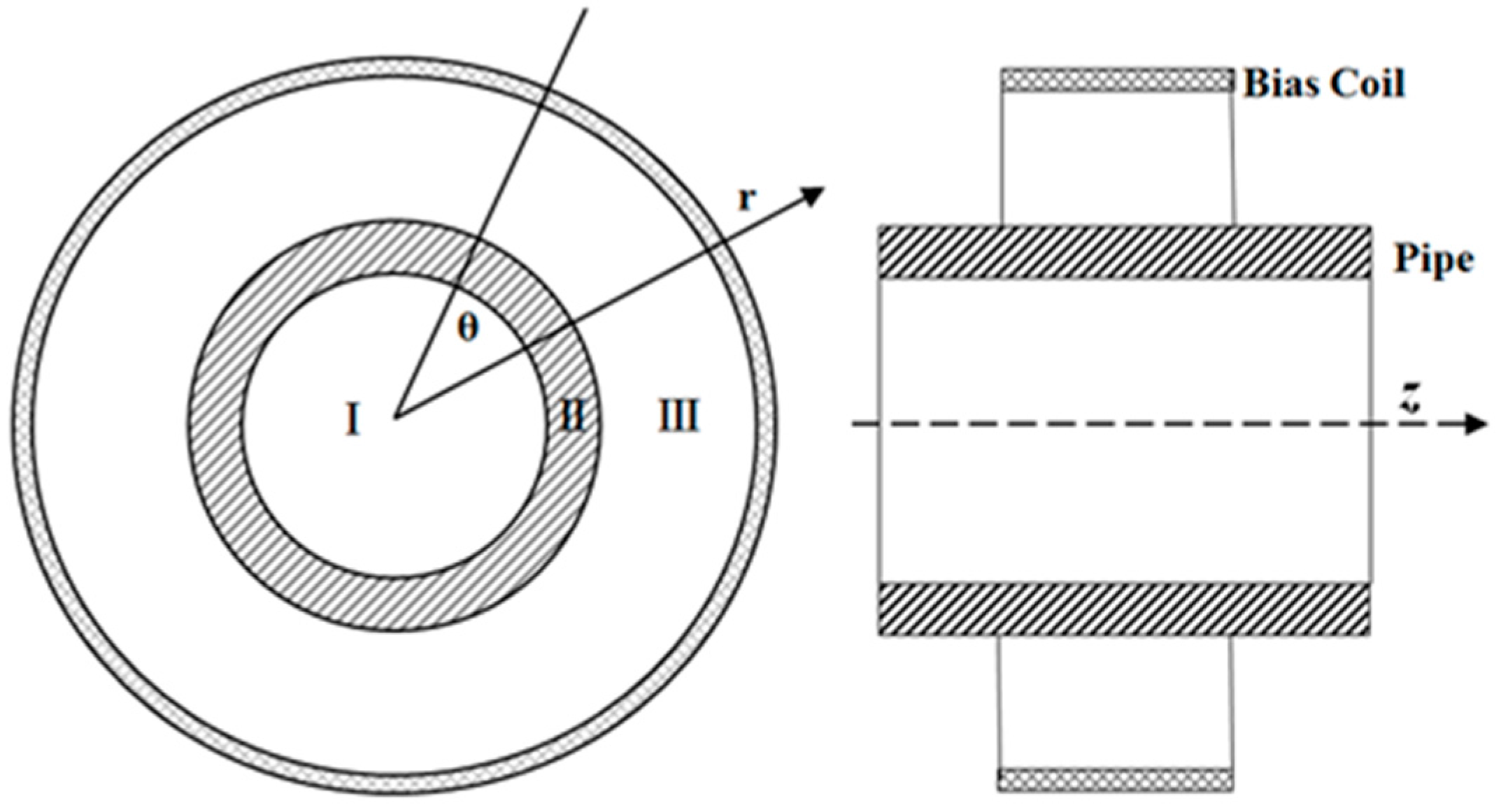
- case 1
- the receiving coil in Zone I:
- case 2
- the receiving coil in Zone III:
4. Experimental Setup
5. Results and Discussions
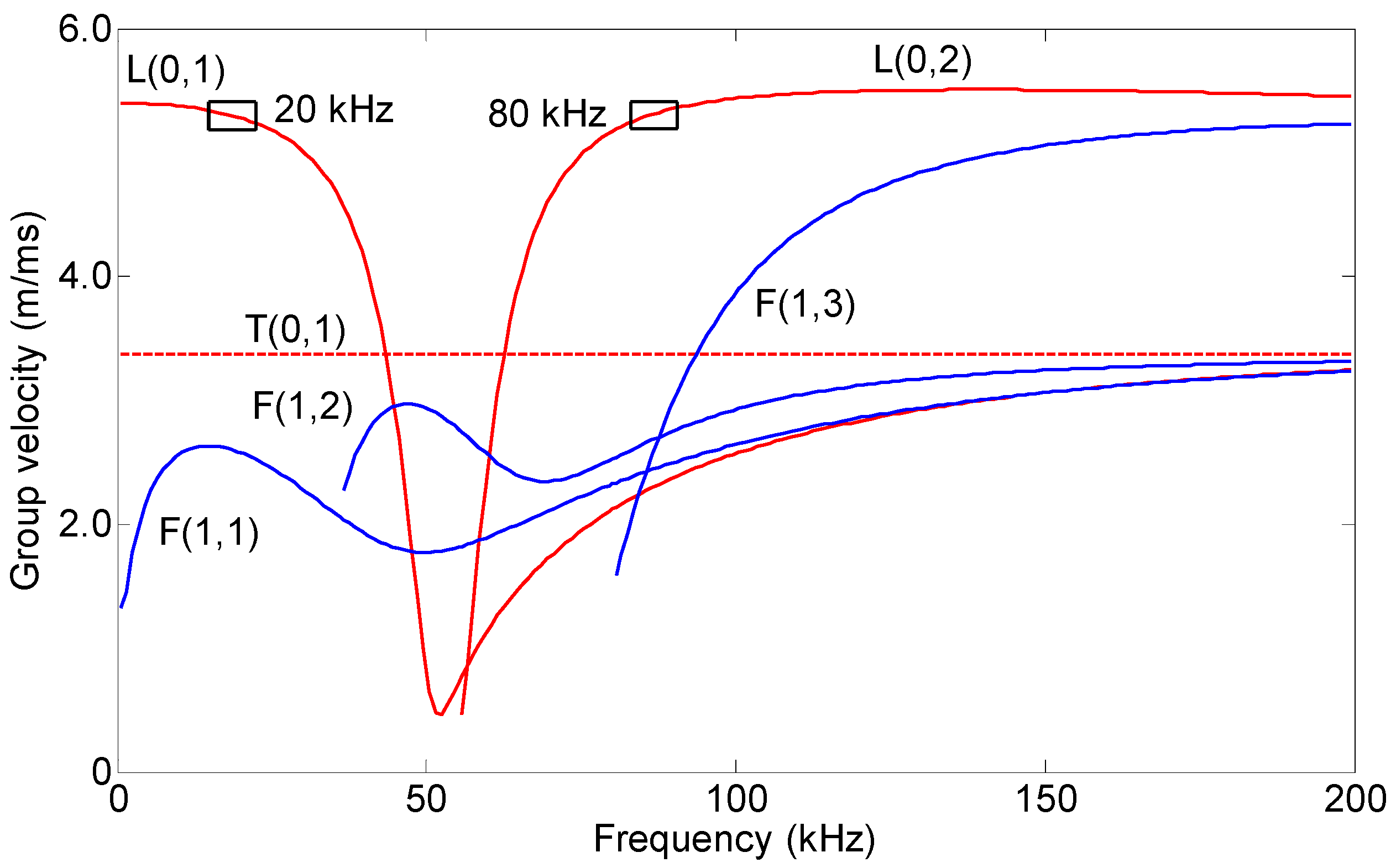
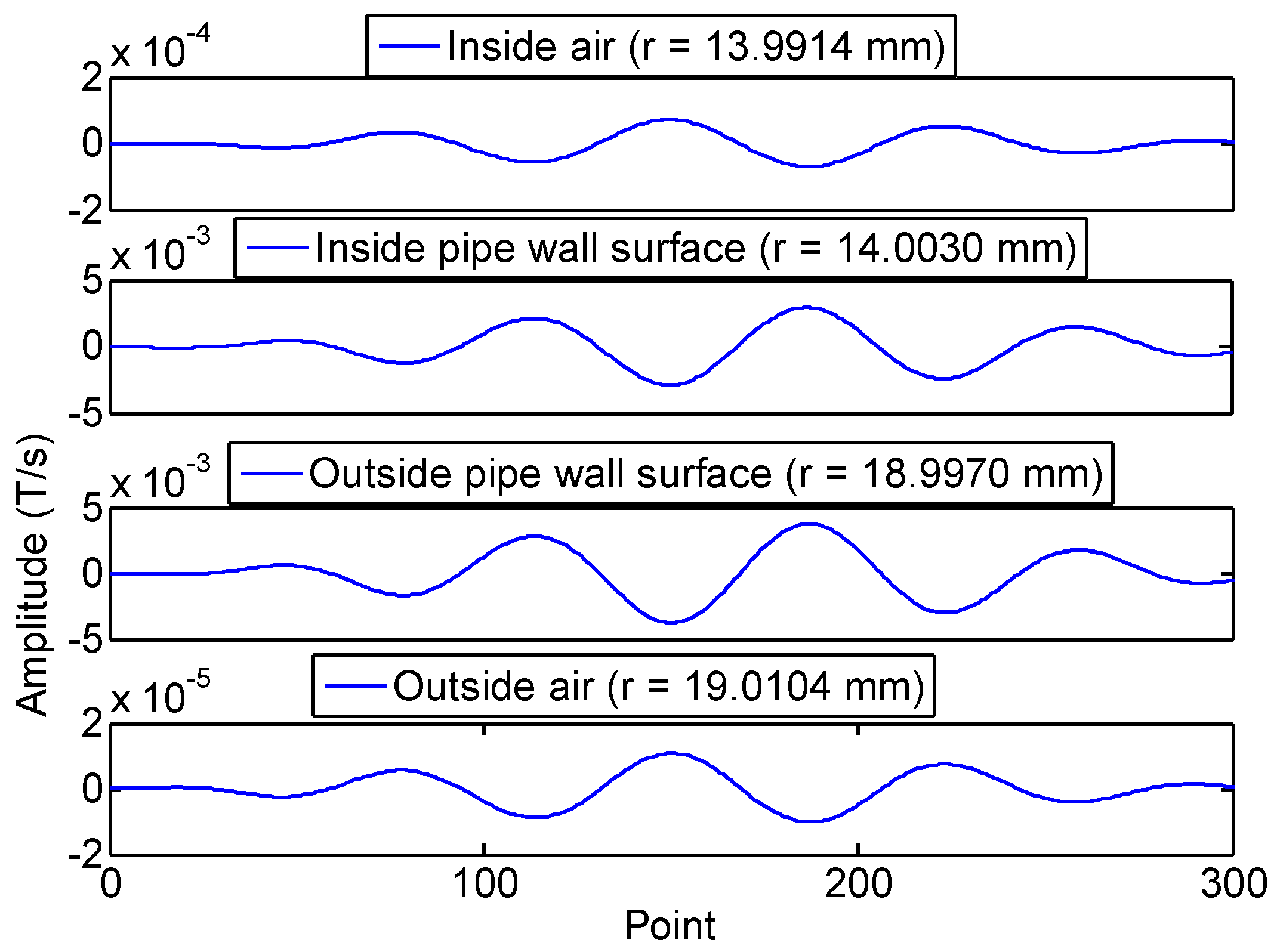
- a)
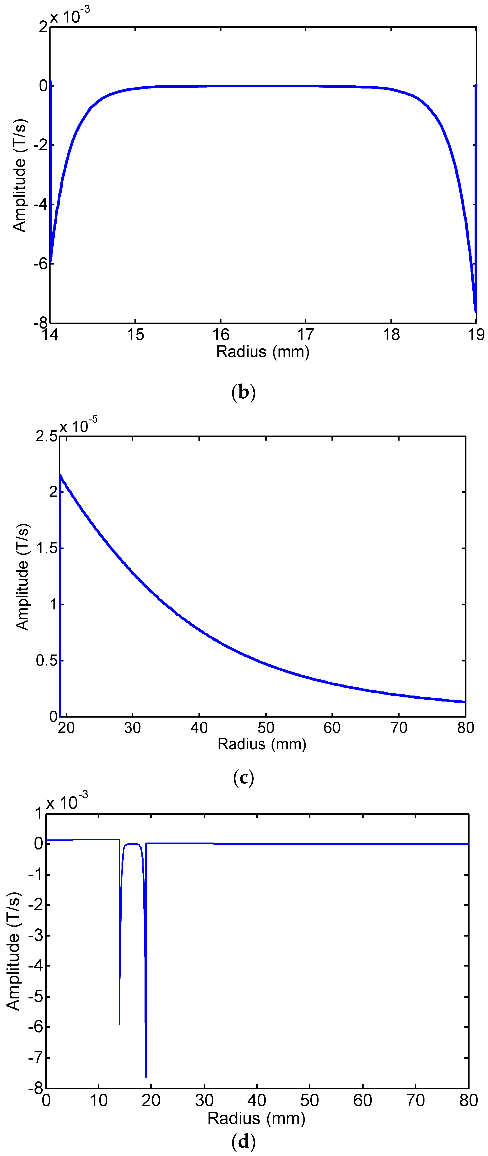
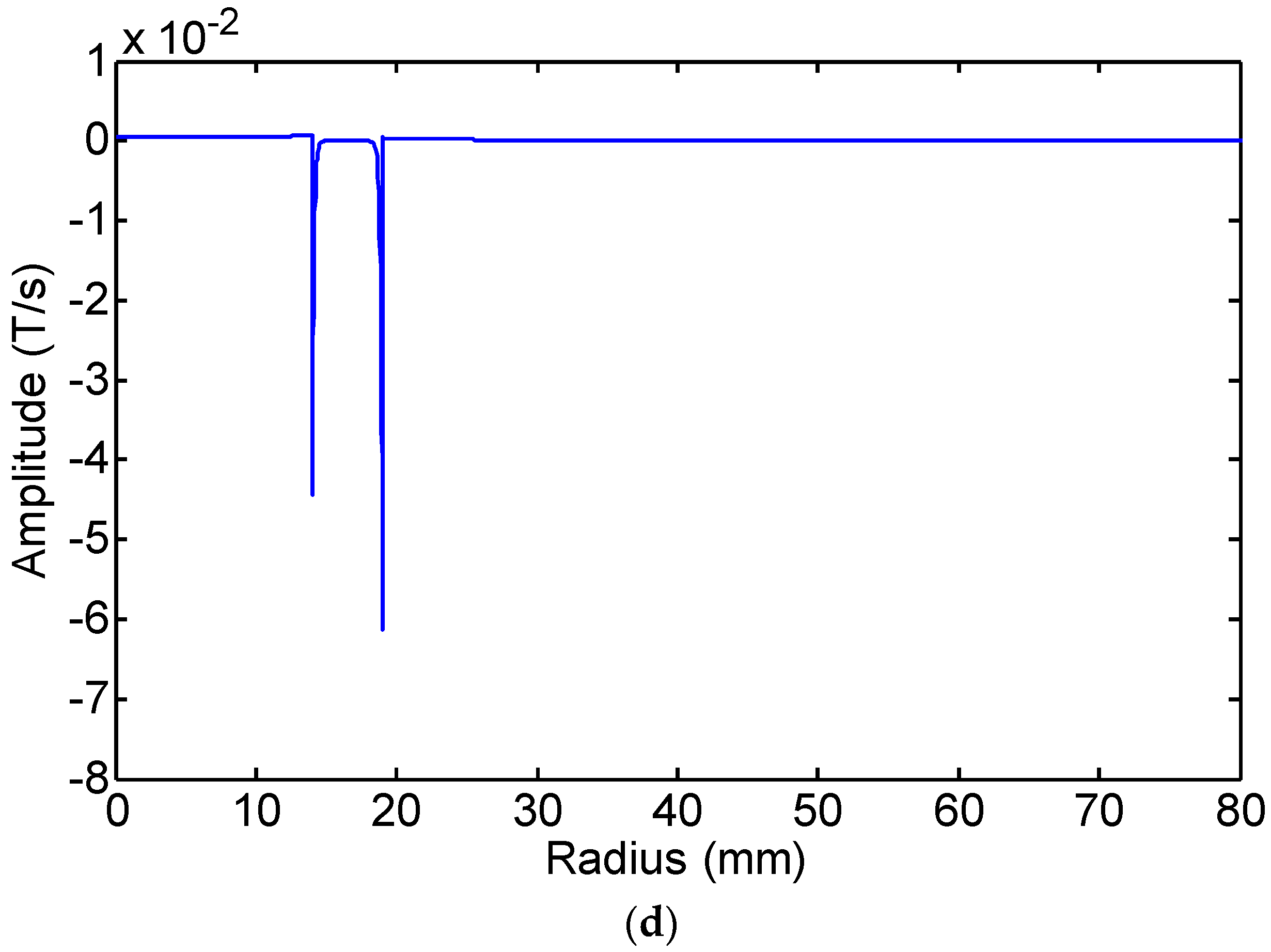
- The magnetic flux density in the pipe wall is concentrated on the internal and external surfaces by the skin effect. The maximum value of the change rate of magnetic flux density in the pipe wall surface is almost two orders of magnitude larger than that of the air zone. The reason is that the permeability of the steel pipe is much greater than that of air.
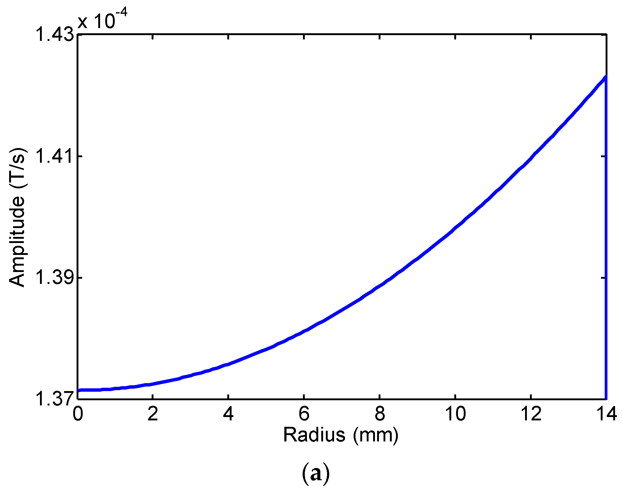
- b)
- The effective area in the pipe wall is very limited, and the magnetic flux density in the pipe wall is decreased quickly due to the skin effect. The magnetic flux density in the pipe wall is very small (dB/dt = −1.686 × 10⁻⁶ T/s, r = 16.5 mm, f = 80 kHz). Although the magnetic flux density in the air zone is less than two orders of magnitude that in the pipe wall, the decay rate of magnetic flux density in the air zone is less than that in the pipe wall. Additionally, the effective area in the air zone is larger than that in the pipe wall.
6. Conclusions
Acknowledgments
Author Contributions
Conflicts of Interest
References
- Kwun, H.; Kim, S.Y.; Light, G.M. The magnetostrictive sensor technology for long range guided wave testing and monitoring of structures. Mater. Eval. 2003, 61, 80–84. [Google Scholar]
- Rizzo, P.; Di Scalea, F.L. Load measurement and health monitoring in cable stays via guided wave magnetostrictive ultrasonics. Mater. Eval. 2004, 62, 1057–1065. [Google Scholar]
- Calkins, F.T.; Flatau, A.B.; Dapino, M.J. Overview of magnetostrictive sensor technology. J. Intell. Mater. Syst. Struct. 2007, 18, 1057–1066. [Google Scholar] [CrossRef]
- Liu, Z.; Zhao, J.; Wu, B.; Zhang, Y.; He, C. Configuration optimization of magnetostrictive transducers for longitudinal guided wave inspection in seven-wire steel strands. NDT E Int. 2010, 43, 484–492. [Google Scholar] [CrossRef]
- Tse, P.; Liu, X.; Liu, Z.; Wu, B.; He, C.; Wang, X. An innovative design for using flexible printed coils for magnetostrictive-based longitudinal guided wave sensors in steel strand inspection. Smart Mater. Struct. 2011, 20, 055001. [Google Scholar] [CrossRef]
- Cobb, A.C.; Kwun, H.; Caseres, L.; Janega, G. Torsional guided wave attenuation in piping from coating, temperature, and large-area corrosion. NDT E Int. 2012, 47, 163–170. [Google Scholar] [CrossRef]
- Panda, A.; Sharan, P.K.; Roy, R.K.; Murthy, G.; Mitra, A. Generation and detection of guided waves in a defective pipe using rapidly quenched magnetostrictive ribbons. Smart Mater. Struct. 2012, 21, 045015. [Google Scholar] [CrossRef]
- Kim, H.W.; Lee, J.K.; Kim, Y.Y. Circumferential phased array of shear-horizontal wave magnetostrictive patch transducers for pipe inspection. Ultrasonics 2013, 53, 423–431. [Google Scholar] [CrossRef] [PubMed]
- Kim, Y.Y.; Kwon, Y.E. Review of magnetostrictive patch transducers and applications in ultrasonic nondestructive testing of waveguides. Ultrasonics 2015, 62, 3–19. [Google Scholar] [CrossRef] [PubMed]
- Liu, Z.; Hu, Y.; Fan, J.; Yin, W.; Liu, X.; He, C.; Wu, B. Longitudinal mode magnetostrictive patch transducer array employing a multi-splitting meander coil for pipe inspection. NDT E Int. 2016, 79, 30–37. [Google Scholar] [CrossRef]
- Jiles, D.C.; Atherton, D.L. Theory of the magnetization process in ferromagnets and its application to the magnetomechanical effect. J. Phys. D Appl. Phys. 1984, 17, 1265–1281. [Google Scholar] [CrossRef]
- Sablik, M.J.; Jiles, D.C. Coupled magnetoelastic theory of magnetic and magnetostrictive hysteresis. IEEE Trans. Magn. 1993, 29, 2113–2123. [Google Scholar] [CrossRef]
- Jiles, D.C. Theory of the magnetomechanical effect. J. Phys. D Appl. Phys. 1995, 28, 1537–1546. [Google Scholar] [CrossRef]
- Naus, H.W.L. Theoretical developments in magnetomechanics. IEEE Trans. Magn. 2011, 47, 2155–2162. [Google Scholar] [CrossRef]
- Li, J.; Xu, M. Modified Jiles-Atherton-Sablik model for asymmetry in magnetomechanical effect under tensile and compressive stress. J. Appl. Phys. 2011, 110, 063918. [Google Scholar] [CrossRef]
- Li, L.; Jiles, D.C. Modified law of approach for the magnetomechanical model: Application of the Rayleigh law to stress. IEEE Trans. Magn. 2003, 39, 3037–3039. [Google Scholar] [CrossRef]
- Dapino, M.J.; Smith, R.C.; Flatau, A.B. Structural magnetic strain model for magnetostrictive transducers. IEEE Trans. Magn. 2000, 36, 545–556. [Google Scholar] [CrossRef]
- Dapino, M.J.; Smith, R.C.; Calkins, F.T.; Flatau, A.B. A coupled magnetomechanical model for magnetostrictive transducers and its application to Villari-effect sensors. J. Intell. Mater. Syst. Struct. 2002, 13, 737–747. [Google Scholar] [CrossRef]
- William, R.C. Theory of magnetostrictive delay lines for pulse and continuous wave transmission. IRE Trans. Ultrason. Eng. 1959, 6, 16–32. [Google Scholar] [CrossRef]
- Lee, H.; Kim, Y.Y. Wave selection using a magnetomechanical sensor in a solid cylinder. J. Acoust. Soc. Am. 2002, 112, 953–960. [Google Scholar] [CrossRef] [PubMed]
- Cho, S.H.; Kim, Y.; Kim, Y.Y. The optimal design and experimental verification of the bias magnet configuration of a magnetostrictive sensor for bending wave measurement. Sens. Actuators A Phys. 2003, 107, 225–232. [Google Scholar] [CrossRef]
- Kim, Y.Y.; Cho, S.H.; Lee, H.C. Application of magnetomechanical sensors for modal testing. J. Sound Vib. 2003, 268, 799–808. [Google Scholar] [CrossRef]
- Han, S.W.; Lee, H.C.; Kim, Y.Y. Noncontact damage detection of a rotating shaft using the magnetostrictive effect. J. Nondestruct. Eval. 2003, 22, 141–150. [Google Scholar] [CrossRef]
- IEEE. IEEE Standard on Magnetostrictive Materials: Piezomagnetic Nomenclature; Std. 319-1990; IEEE Std.: New York, NY, USA, 1991; p. 9. [Google Scholar]
- Pavlakovic, B.; Lowe, M.; Alleyne, D.; Cawley, P. Disperse: A general purpose program for creating dispersion curves. In Review of Progress in Quantitative Nondestructive Evaluation; Thompson, D.O., Chimenti, D.E., Eds.; Springer US: New York, NY, USA, 1997; pp. 185–192. [Google Scholar]
- Thompson, R.B. A model for the electromagnetic generation of ultrasonic guided waves in ferromagnetic metal polycrystals. IEEE Trans. Sonics Ultrason. 1978, 25, 7–15. [Google Scholar] [CrossRef]
- Xu, J.; Wu, X.; Kong, D.; Sun, P. A guided wave sensor based on the inverse magnetostrictive effect for distinguishing symmetric from asymmetric features in pipes. Sensors 2015, 15, 5151–5162. [Google Scholar] [CrossRef] [PubMed]


| Object | Parameters | Symbol | Value |
|---|---|---|---|
| Pipe | Inner radius | r1 | 14 mm |
| Outer radius | r2 | 19 mm | |
| Conductivity | σ | 1.12 × 10⁷ S/m | |
| Youngs Modulus | E | 210 GPa | |
| Poissons ratio | ν | 0.29 | |
| Density | ρ | 7870 kg/m3 | |
| Bias coil | Width | wb | 110 mm |
| Height | hb | 5 mm | |
| Inside diameter | IDb | 160 mm | |
| Turns number | Nb | 500 | |
| Conductivity | σ | 6.7 × 10⁷ S/m | |
| Permeability | urc | 1 | |
| Excitation coil | Width | wT | 11 mm |
| Height | hT | 0.5 mm | |
| Liftoff | lf | 0.25 mm | |
| Turns number | NT | 20 | |
| Conductivity | σ | 6.7 × 10⁷ S/m | |
| Permeability | urc | 1 | |
| Excitation parameters | Amplitude | I | 5 A |
| Center frequency | f | 20 kHz, 80 kHz | |
| Receiving coil | Width | wR | 11 mm |
| Height | hR | 0.5 mm | |
| Turns number | NR | 20 |
© 2016 by the authors; licensee MDPI, Basel, Switzerland. This article is an open access article distributed under the terms and conditions of the Creative Commons Attribution (CC-BY) license (http://creativecommons.org/licenses/by/4.0/).
Share and Cite
Xu, J.; Sun, Y.; Zhou, J. Research on the Lift-off Effect of Receiving Longitudinal Mode Guided Waves in Pipes Based on the Villari Effect. Sensors 2016, 16, 1529. https://doi.org/10.3390/s16091529
Xu J, Sun Y, Zhou J. Research on the Lift-off Effect of Receiving Longitudinal Mode Guided Waves in Pipes Based on the Villari Effect. Sensors. 2016; 16(9):1529. https://doi.org/10.3390/s16091529
Chicago/Turabian StyleXu, Jiang, Yong Sun, and Jinhai Zhou. 2016. "Research on the Lift-off Effect of Receiving Longitudinal Mode Guided Waves in Pipes Based on the Villari Effect" Sensors 16, no. 9: 1529. https://doi.org/10.3390/s16091529