On Event-Triggered Adaptive Architectures for Decentralized and Distributed Control of Large-Scale Modular Systems

Abstract

The last decade has witnessed an increased interest in physical systems controlled over wireless networks (networked control systems). These systems allow the computation of control signals via processors that are not attached to the physical systems, and the feedback loops are closed over wireless networks. The contribution of this paper is to design and analyze event-triggered decentralized and distributed adaptive control architectures for uncertain networked large-scale modular systems; that is, systems consist of physically-interconnected modules controlled over wireless networks. Specifically, the proposed adaptive architectures guarantee overall system stability while reducing wireless network utilization and achieving a given system performance in the presence of system uncertainties that can result from modeling and degraded modes of operation of the modules and their interconnections between each other. In addition to the theoretical findings including rigorous system stability and the boundedness analysis of the closed-loop dynamical system, as well as the characterization of the effect of user-defined event-triggering thresholds and the design parameters of the proposed adaptive architectures on the overall system performance, an illustrative numerical example is further provided to demonstrate the efficacy of the proposed decentralized and distributed control approaches.

1. Introduction

The design and implementation of decentralized and distributed architectures for controlling complex, large-scale systems is a nontrivial control engineering task involving the consideration of components interacting with the physical processes to be controlled. In particular, large-scale systems are characterized by a large number of highly coupled components exchanging matter, energy or information and have become ubiquitous given the recent advances in embedded sensor and computation technologies. Examples of such systems include, but are not limited to, multi-vehicle systems, communication systems, power systems, process control systems and water systems (see, for example, [1,2,3,4,5,6] and the references therein). This paper concentrates on an important class of large-scale systems; namely, large-scale modular systems that consist of physically-interconnected and generally heterogeneous modules.

1.1. Motivation and Literature Review

Two sweeping generalizations can be made about large-scale modular systems. The first is that their complex structure and large-scale nature yield to inaccurate mathematical module models, since it is a challenge to precisely model each module of a large-scale system and the interconnections between these modules. As a consequence, the discrepancies between the modules and their mathematical models, that is system uncertainties, result in the degradation of overall system stability and the performance of the large-scale modular systems. To this end, adaptive control methodologies [7,8,9,10,11,12,13] offer an important capability for this class of dynamical systems to learn and suppress the effect of system uncertainties resulting from modeling and degraded modes of operation, and hence, they offer system stability and desirable closed-loop system performance in the presence of system uncertainties without excessively relying on mathematical models.

The second generalization about large-scale modular systems is that these systems are often controlled over wireless networks, and hence, the communication costs between the modules and their remote processors increase proportionally with the increase in the number of modules and often the interconnection between these modules. To this end, event-triggered control methodologies [14,15,16] offer new control execution paradigms that relax the fixed periodic demand of computational resources and allow for the aperiodic exchange of sensor and actuator information with the remote processor to reduce overall communication cost over a wireless network. Note that adaptive control methodologies and event-triggered control methodologies are often studied separately in the literature, where it is of practical importance to theoretically integrate these two approaches to guarantee system stability and the desirable closed-loop system performance of uncertain large-scale modular systems with reduced communication costs over wireless networks, which is the main focus of this paper.

More specifically, the authors of [6,17,18,19,20,21,22,23] proposed decentralized and distributed adaptive control architectures for large-scale systems; however, these approaches do not make any attempts to reduce the overall communication cost over wireless networks using, for example, event-triggered control methodologies. In addition, the authors of [24,25,26,27,28,29,30] present decentralized and distributed control architectures with event triggering; however, these approaches do not consider adaptive control architectures and assume perfect models of the processes to be controlled; hence, they are not practical for large-scale modular systems with significant system uncertainties. Only the authors of [31,32,33,34,35,36] present event-triggered adaptive control approaches for uncertain dynamical systems. In particular, the authors of [31,32] consider data transmission from a physical system to the controller, but not vice versa, while developing their adaptive control approaches to deal with system uncertainties. On the other hand, the adaptive control architectures of the authors in [33,34,35,36] consider two-way data transmission over wireless networks; that is, from a physical system to the controller and from the controller to this physical system. However, none of these approaches can be directly applied to large-scale modular systems. This is due to the fact that large-scale modular systems require decentralized and distributed architectures, and direct application of the results in [31,32,33,34,35,36] to this class of systems can result in centralized architectures, which is not practically desired due to the large-scale nature of modular systems. To summarize, there do not exist resilient adaptive control architectures for large-scale systems in the literature to deal with system uncertainties while reducing the communication costs between the models and their remote processors.

1.2. Contribution

The contribution of this paper is to design and analyze event-triggered decentralized and distributed adaptive control architectures for uncertain large-scale systems controlled over wireless networks. Specifically, the proposed decentralized and distributed adaptive architectures of this paper guarantee overall system stability while reducing wireless network utilization and achieving a given system performance in the presence of system uncertainties that can result from modeling and degraded modes of operation of the modules and their interconnections between each other. From a theoretical viewpoint, the proposed event-triggered adaptive architectures here can be viewed as a significant generalization of our prior work documented in [35,36] to large-scale modular systems, which consider a state emulator-based adaptive control methodology with robustness against high-frequency oscillations in the controller response [10,13,37,38,39,40,41,42]. In this generalization, we also adopt necessary tools and methods from [6,23] on decentralized and distributed adaptive controller construction for large-scale modular systems. In addition to the theoretical findings including rigorous system stability and boundedness analysis of the closed-loop dynamical system and the characterization of the effect of user-defined event-triggering thresholds, as well as the design parameters of the proposed adaptive architectures on the overall system performance, an illustrative numerical example is further provided to demonstrate the efficacy of the proposed decentralized and distributed control approaches.

1.3. Organization

The contents of the paper are as follows. In Section 2, we consider an event-triggered decentralized adaptive control approach for large-scale modular systems, where the considered approach assumes that physically-interconnected modules cannot communicate with each other for exchanging their state information. Specifically, Theorem 1 and Corollaries 1–4 show the main results of Section 2 subject to some structural conditions on the parameters of the large-scale modular systems and the proposed event-triggered decentralized control architecture (see Assumptions 4 and 5). In Section 3, we consider an event-triggered distributed adaptive control approach in Theorem 2 and Corollaries 5–7 for getting rid of such structural conditions, where the considered approach assumes that physically-interconnected modules can locally communicate with each other for exchanging their state information. Finally, the illustrative numerical example is presented in Section 4, and conclusions are summarized in Section 5.

1.4. Notation

The notation used in this paper is fairly standard. Specifically, $\mathbb{R}$ denotes the set of real numbers; ${\mathbb{R}}^n$ denotes the set of $n\times 1$ real column vectors; ${\mathbb{R}}^{n\times m}$ denotes the set of $n\times m$ real matrices; ${\mathbb{R}}_{+}$ denotes the set of positive real numbers; ${\mathbb{R}}_{+}^{n\times n}$ denotes the set of $n\times n$ positive-definite real matrices; ${\mathbb{S}}^{n\times n}$ denotes the set of $n\times n$ symmetric real matrices; ${\mathbb{D}}^{n\times n}$ denotes the set of $n\times n$ real matrices with diagonal scalar entries; ${(·)}^{\mathrm{T}}$ denotes transpose; ${(·)}^{-1}$ denotes inverse; $\mathrm{tr}(·)$ denotes the trace operator; $\text{diag}\left(a\right)$ denotes the diagonal matrix with the vector a on its diagonal; and “≜” denotes equality by definition. In addition, we write ${\lambda }_{\text{min}}\left(A\right)$ (respectively, ${\lambda }_{\text{max}}\left(A\right))$ for the minimum and respectively maximum eigenvalue of the Hermitian matrix A, $\parallel ·\parallel$ for the Euclidean norm and ${\parallel ·\parallel }_{\mathrm{F}}$ for the Frobenius matrix norm. Furthermore, we use “∨” for the “or” logic operator and “$\overline{(·)}$” for the “not” logic operator.

We adopt graphs [43] to encode physical interactions and communications between modules. In particular, an undirected graph $\mathcal{G}$ is defined by ${\mathcal{V}}_{\mathcal{G}}=\left\{1,\cdots ,N\right\}$ of nodes and a set ${\mathcal{E}}_{\mathcal{G}}\in {\mathcal{V}}_{\mathcal{G}}\times {\mathcal{V}}_{\mathcal{G}}$ of edges. If $(i,j)\in {\mathcal{E}}_{\mathcal{G}},$ then the nodes i and j are neighbors, and the neighboring relation is indicated with $i\sim j$. The degree of a node is given by the number of its neighbors, where $d_i$ denotes the degree of node i. Lastly, the adjacency matrix of a graph $\mathcal{G}$, $\mathcal{A}\left(\mathcal{G}\right)\in {\mathbb{R}}^{N\times N}$, is given by:

$${\left[\mathcal{A}\left(\mathcal{G}\right)\right]}_{ij}\triangleq \left\{\begin{array}{cc}& 1,\text{if}(i,j)\in {\mathcal{E}}_{\mathcal{G}}\hfill \\ & 0,\text{otherwise}\hfill \end{array}\right.$$

(1)

2. Event-Triggered Decentralized Adaptive Control

In this section, we introduce an event-triggered decentralized adaptive control architecture, where it is assumed that physically-interconnected modules cannot communicate with each other. For organizational purposes, this section is broken up into two subsections. Specifically, we first briefly overview a standard decentralized adaptive control architecture without event-triggering and then present the proposed event-triggered decentralized adaptive control approach, which includes rigorous stability and performance analyses with no Zeno behavior and generalizations to the state emulator case for suppressing the effect of possible high-frequency oscillations in the controller response.

2.1. Overview of a Standard Decentralized Adaptive Control Architecture without Event-Triggering

Consider an uncertain large-scale modular system $\mathcal{S}$ consisting of N interconnected modules ${\mathcal{S}}_i$, $i\in {\mathcal{V}}_{\mathcal{G}}$, given by:

$${\mathcal{S}}_i:{\dot{x}}_i\left(t\right)=A_i{x}_i\left(t\right)+B_i\left[{\mathrm{\Lambda }}_i{u}_i\left(t\right)+{\Delta }_i\left(x_i\left(t\right)\right)+\sum _{i\sim j}{\delta }_{ij}\left(x_j\left(t\right)\right)\right],x_i\left(0\right)=x_{i0}$$

(2)

where $x_i\left(t\right)\in {\mathbb{R}}^{n_i}$ is the state of ${\mathcal{S}}_i$, $u_i\left(t\right)\in {\mathbb{R}}^{m_i}$ is the control input applied to ${\mathcal{S}}_i$, $A_i\in {\mathbb{R}}^{n_i\times n_i}$, $B_i\left(t\right)\in {\mathbb{R}}^{n_i\times m_i}$ are known matrices and the pair $\left(A_i,B_i\right)$ is controllable. In addition, ${\mathrm{\Lambda }}_i\in {\mathbb{R}}_{+}^{m_i\times m_i}\cap {\mathbb{D}}^{m_i\times m_i}$ is an unknown module control effectiveness matrix; ${\Delta }_i:{\mathbb{R}}^{n_i}\to {\mathbb{R}}^{m_i}$ represents matched module bounded uncertainties; and ${\delta }_{ij}:{\mathbb{R}}^{n_j}\to {\mathbb{R}}^{m_i}$ represents matched unknown physical interconnections with respect to module j, $j\in {\mathcal{V}}_{\mathcal{G}}$, such that $(i,j)\in {\mathcal{E}}_{\mathcal{G}}$.

Assumption 1. 

The unknown module uncertainty is parameterized as:

$$\begin{array}{c}\hfill {\Delta }_i\left(x_i\left(t\right)\right)=W_{\mathrm{o}i}^{\mathrm{T}}{\beta }_i\left(x_i\left(t\right)\right),x_i\in {\mathbb{R}}^{n_i}\end{array}$$

(3)

where $W_{oi}\in {\mathbb{R}}^{g_i\times m_i}$ is an unknown weight matrix, which satisfies $\parallel W_{oi}{\parallel }_F\le {\omega }_i^{*}$, ${\omega }_i^{*}\in {\mathbb{R}}_{+}$, and ${\beta }_i\left(x_i\left(t\right)\right):{\mathbb{R}}^{n_i}\to {\mathbb{R}}^{g_i}$ is a known Lipschitz continuous basis function vector satisfying:

$$\begin{array}{c}\hfill \parallel {\beta }_i\left(x_{1i}\right)-{\beta }_i\left(x_{2i}\right)\parallel \le L_{\beta i}\parallel x_{1i}-x_{2i}\parallel \end{array}$$

(4)

with $L_{\beta i}\in {\mathbb{R}}_{+}$.

Assumption 2. 

The function ${\delta }_{ij}\left(x_j\left(t\right)\right)$ in Equation (2) satisfies:

$$\begin{array}{c}\hfill \parallel {\delta }_{ij}\left(x_j\left(t\right)\right)\parallel \le {\alpha }_{ij}\parallel x_j\left(t\right)\parallel ,{\alpha }_{ij}>0,x_j\in {\mathbb{R}}^{n_j}\end{array}$$

(5)

Next, consider the reference model ${\mathcal{S}}_{\mathrm{r}i}$ capturing a desired closed-loop performance for module i, $i\in {\mathcal{V}}_{\mathcal{G}}$ given by:

$$\begin{array}{c}\hfill {\mathcal{S}}_{\mathrm{r}i}:{\dot{x}}_{\mathrm{r}i}\left(t\right)=A_{\mathrm{r}i}{x}_{\mathrm{r}i}\left(t\right)+B_{\mathrm{r}i}{c}_i\left(t\right),x_{\mathrm{r}i}\left(0\right)=x_{\mathrm{r}i0}\end{array}$$

(6)

where $x_{\mathrm{r}i}\left(t\right)\in {\mathbb{R}}^{n_i}$ is the reference state vector of ${\mathcal{S}}_{\mathrm{r}i}$, $c_i\left(t\right)\in {\mathbb{R}}^{m_i}$ is a given bounded command of ${\mathcal{S}}_{\mathrm{r}i}$, $A_{\mathrm{r}i}\in {\mathbb{R}}^{n_i\times n_i}$ is the reference system matrix and $B_{\mathrm{r}i}\in {\mathbb{R}}^{n_i\times m_i}$ is the command input matrix.

Assumption 3. 

There exist $K_{1i}\in {\mathbb{R}}^{m_i\times n_i}$ and $K_{2i}\in {\mathbb{R}}^{m_i\times m_i}$, such that $A_{\mathrm{r}i}=A_i-B_i{K}_{1i}$ and $B_{\mathrm{r}i}=B_i{K}_{2i}$ hold with $A_{\mathrm{r}i}$ being Hurwitz.

Using Assumptions 1 and 3, Equation (2) can be equivalently written as:

$$\begin{array}{c}\hfill {\dot{x}}_i\left(t\right)=A_{\mathrm{r}i}{x}_i\left(t\right)+B_{\mathrm{r}i}{c}_i\left(t\right)+B_i{\mathrm{\Lambda }}_i\left[u_i\left(t\right)+W_i^{\mathrm{T}}{\sigma }_i\left(x_i\left(t\right),c_i\left(t\right)\right)\right]+B_i\sum _{i\sim j}{\delta }_{ij}\left(x_j\left(t\right)\right)\end{array}$$

(7)

where $W_i\triangleq {\left[{\mathrm{\Lambda }}_i^{-1}{W}_{\mathrm{o}i}^{\mathrm{T}},{\mathrm{\Lambda }}_i^{-1}{K}_{1i}^{\mathrm{T}},{\mathrm{\Lambda }}_i^{-1}{K}_{2i}^{\mathrm{T}}\right]}^{\mathrm{T}}\in {\mathbb{R}}^{(g_i+n_i+m_i)\times m_i}$ is the unknown weight matrix and ${\sigma }_i\left(x_i\left(t\right),c_i\left(t\right)\right)\triangleq {\left[{\beta }_i^{\mathrm{T}}\left(x_i\left(t\right)\right),x_i^{\mathrm{T}}\left(t\right),c_i^{\mathrm{T}}\left(t\right)\right]}^{\mathrm{T}}\in {\mathbb{R}}^{g_i+n_i+m_i}$. Motivated from the structure of the uncertain terms appearing in Equation (7), let the decentralized adaptive feedback controller of ${\mathcal{S}}_i,i\in {\mathcal{V}}_{\mathcal{G}}$, be given by:

$$\begin{array}{c}\hfill {\mathcal{C}}_i:u_i\left(t\right)\triangleq -{\widehat{W}}_i{\left(t\right)}^{\mathrm{T}}{\sigma }_i\left(x_i\left(t\right),c_i\left(t\right)\right)\end{array}$$

(8)

where ${\widehat{W}}_i\left(t\right)$ is an estimate of $W_i$ satisfying the update law:

$$\begin{array}{c}\hfill {\dot{\widehat{W}}}_i\left(t\right)\triangleq {\gamma }_i{\mathrm{Proj}}_{\mathrm{m}}[{\widehat{W}}_i\left(t\right),{\sigma }_i\left(x_i\left(t\right),c_i\left(t\right)\right){\left(x_i\left(t\right)-x_{ri}\left(t\right)\right)}^{\mathrm{T}}{P}_i{B}_i],{\widehat{W}}_i\left(0\right)={\widehat{W}}_{i0}\end{array}$$

(9)

where ${\mathrm{Proj}}_{\mathrm{m}}$ denotes the projection operator defined for matrices [10,35,44,45], ${\gamma }_i\in {\mathbb{R}}_{+}$ being the learning rate and $P_i\in {\mathbb{R}}_{+}^{n_i\times n_i}\cap {\mathbb{S}}^{n_i\times n_i}$ being a solution of the Lyapunov equation:

$$\begin{array}{c}\hfill 0=A_{\mathrm{r}i}^{\mathrm{T}}{P}_i+P_i{A}_{\mathrm{r}i}+R_i\end{array}$$

(10)

with $R_i\in {\mathbb{R}}_{+}^{n_i\times n_i}\cap {\mathbb{S}}^{n_i\times n_i}$. Now, letting:

$$\begin{array}{cc}\hfill e_i\left(t\right)& \triangleq x_i\left(t\right)-x_{\mathrm{r}i}\left(t\right)\hfill \end{array}$$

(11)

$$\begin{array}{cc}\hfill {\tilde{W}}_i\left(t\right)& \triangleq {\widehat{W}}_i\left(t\right)-W_i\hfill \end{array}$$

(12)

and using Equations (6) and (7), the module-level closed-loop error dynamics are given by:

$$\begin{array}{c}\hfill {\dot{e}}_i\left(t\right)=A_{\mathrm{r}i}{e}_i\left(t\right)-B_i{\mathrm{\Lambda }}_i{\tilde{W}}_i^{\mathrm{T}}\left(t\right){\sigma }_i\left(x_i\left(t\right),c_i\left(t\right)\right)+B_i\sum _{i\sim j}{\delta }_{ij}\left(x_j\left(t\right)\right),e_i\left(t\right)=e_{i0}\end{array}$$

(13)

2.2. Proposed Event-Triggered Decentralized Adaptive Control Architecture

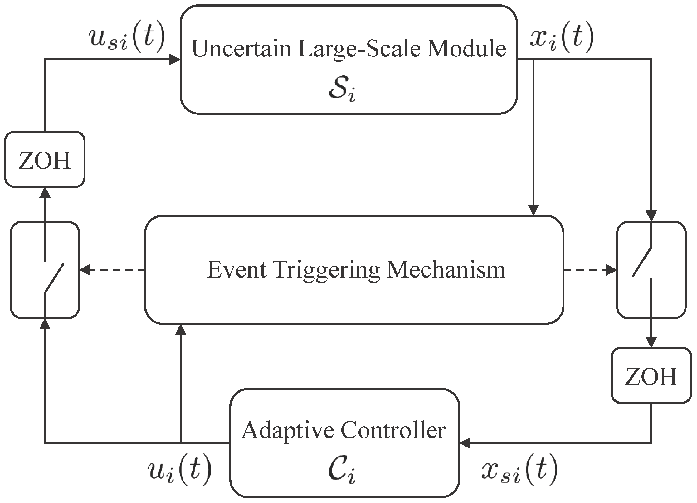
We now present the proposed event-triggered decentralized adaptive control architecture for large-scale modular systems, which reduces wireless network utilization and allows a desirable command tracking performance during the two-way data exchange between the module ${\mathcal{S}}_i$, $i\in {\mathcal{V}}_{\mathcal{G}}$, and its local controller ${\mathcal{C}}_i$, over a wireless network. For this objective, we utilize event-triggering control theory to schedule the data exchange dependent on errors exceeding user-defined thresholds. Specifically, the module sends its state signal to its local adaptive controller only when a predefined event occurs. The $k_i$-th time instants of the state transmission of the module are represented by the monotonic sequence ${\left\{s_{k_i}\right\}}_{k_i=1}^{\infty }$, where $s_{k_i}\in {\mathbb{R}}_{+}$. The local controller uses this triggered module state signal to compute the control signal using adaptive control architecture. In addition, the local controller sends the updated feedback control input to the module only when another predefined event occurs. The $j_i$-th time instants of the feedback control transmission are then represented by the monotonic sequence ${\left\{r_{j_i}\right\}}_{j_i=1}^{\infty }$, where $r_{j_i}\in {\mathbb{R}}_{+}$. As depicted in Figure 1, each module state signal and its local control input are held by a zero-order-hold operator (ZOH) until the next triggering event for the corresponding signal takes place. The delay in sampling, data transmission and computation is not considered in this paper. Consider the uncertain dynamical module i given by:

$$\begin{array}{c}\hfill {\mathcal{S}}_i:{\dot{x}}_i\left(t\right)=A_i{x}_i\left(t\right)+B_i\left[{\mathrm{\Lambda }}_i{u}_{\mathrm{s}i}\left(t\right)+{\Delta }_i\left(x_i\left(t\right)\right)+\sum _{i\sim j}{\delta }_{ij}\left(x_j\left(t\right)\right)\right],x_i\left(0\right)=x_{i0}\end{array}$$

(14)

where $u_{\mathrm{s}i}\left(t\right)\in {\mathbb{R}}^{m_i}$ is the sampled control input vector. Using Assumptions 1 and 3, Equation (14) can be equivalently written as:

$$\begin{array}{ccc}\hfill {\dot{x}}_i\left(t\right)& =& A_{\mathrm{r}i}{x}_i\left(t\right)+B_{\mathrm{r}i}{c}_i\left(t\right)+B_i{\mathrm{\Lambda }}_i\left[u_{\mathrm{s}i}\left(t\right)+W_i^{\mathrm{T}}{\sigma }_i\left(x_i\left(t\right),x_{\mathrm{s}i}\left(t\right),c_i\left(t\right)\right)\right]+B_i\sum _{i\sim j}{\delta }_{ij}\left(x_j\left(t\right)\right)\hfill \\ & & +B_i{\mathrm{\Lambda }}_i(u_{\mathrm{s}i}\left(t\right)-u_i\left(t\right))+B_i{K}_{1i}(x_{\mathrm{s}i}\left(t\right)-x_i\left(t\right))\hfill \end{array}$$

(15)

where $x_{\mathrm{s}i}\left(t\right)\in {\mathbb{R}}^{n_i}$ is the sampled state vector, ${\sigma }_i\left(x_i\left(t\right),x_{\mathrm{s}i}\left(t\right),c_i\left(t\right)\right)\triangleq {\left[{\beta }_i^{\mathrm{T}}\left(x_i\left(t\right)\right),x_{\mathrm{s}i}^{\mathrm{T}}\left(t\right),c_i^{\mathrm{T}}\left(t\right)\right]}^{\mathrm{T}}\in {\mathbb{R}}^{g_i+n_i+m_i}$. Now, let the adaptive feedback control law be given by:

$$\begin{array}{c}\hfill {\mathcal{C}}_i:u_i\left(t\right)=-{\widehat{W}}_i{\left(t\right)}^{\mathrm{T}}{\sigma }_i\left(x_{\mathrm{s}i}\left(t\right),c_i\left(t\right)\right)\end{array}$$

(16)

where ${\sigma }_i\left(x_{\mathrm{s}i}\left(t\right),c_i\left(t\right)\right)=[{\beta }_i^{\mathrm{T}}\left(x_{\mathrm{s}i}\left(t\right)\right),x_{\mathrm{s}i}^{\mathrm{T}}\left(t\right),c_i^{\mathrm{T}}\left(t\right){]}^{\mathrm{T}}\in {\mathbb{R}}^{g_i+n_i+m_i}$, and ${\widehat{W}}_i\left(t\right)$ satisfies the weight update law:

$$\begin{array}{c}\hfill {\dot{\widehat{W}}}_i\left(t\right)={\gamma }_i{\mathrm{Proj}}_{\mathrm{m}}[{\widehat{W}}_i\left(t\right),{\sigma }_i\left(x_{\mathrm{s}i}\left(t\right),c_i\left(t\right)\right)e_{\mathrm{s}i}^{\mathrm{T}}\left(t\right)P_i{B}_i],{\widehat{W}}_i\left(0\right)={\widehat{W}}_{i0}\end{array}$$

(17)

with $e_{\mathrm{s}i}\left(t\right)\triangleq x_{\mathrm{s}i}\left(t\right)-x_{\mathrm{r}i}\left(t\right)\in {\mathbb{R}}^{n_i}$ being the error of the triggered module state vector. Note that using Equation (16), Equation (15) can be rewritten as:

$$\begin{array}{cc}\hfill {\dot{x}}_i\left(t\right)=& A_{\mathrm{r}i}{x}_i\left(t\right)+B_{\mathrm{r}i}{c}_i\left(t\right)-B_i{\mathrm{\Lambda }}_i{\tilde{W}}_i^{\mathrm{T}}\left(t\right){\sigma }_i\left(x_{\mathrm{s}i}\left(t\right),c_i\left(t\right)\right)-B_i{\mathrm{\Lambda }}_i{g}_i(·)+B_i\sum _{i\sim j}{\delta }_{ij}\left(x_j\left(t\right)\right)\hfill \\ & +B_i{\mathrm{\Lambda }}_i(u_{\mathrm{s}i}\left(t\right)-u_i\left(t\right))+B_i{K}_{1i}(x_{\mathrm{s}i}\left(t\right)-x_i\left(t\right))\hfill \end{array}$$

(18)

where $g_i(·)\triangleq W_i^{\mathrm{T}}\left[{\sigma }_i\left(x_{\mathrm{s}i}\left(t\right),c_i\left(t\right)\right)-{\sigma }_i\left(x_i\left(t\right),x_{\mathrm{s}i}\left(t\right),c_i\left(t\right)\right)\right]$, and using Equations (18) and (6), we can write the module error dynamics as:

$$\begin{array}{cc}\hfill {\dot{e}}_i\left(t\right)=& A_{\mathrm{r}i}{e}_i\left(t\right)-B_i{\mathrm{\Lambda }}_i{\tilde{W}}_i^{\mathrm{T}}\left(t\right){\sigma }_i\left(x_{\mathrm{s}i}\left(t\right),c_i\left(t\right)\right)-B_i{\mathrm{\Lambda }}_i{g}_i(·)+B_i\sum _{i\sim j}{\delta }_{ij}\left(x_j\left(t\right)\right)+B_i{\mathrm{\Lambda }}_i(u_{\mathrm{s}i}\left(t\right)-u_i\left(t\right))\hfill \\ & +B_i{K}_{1i}(x_{\mathrm{s}i}\left(t\right)-x_i\left(t\right))\hfill \end{array}$$

(19)

The proposed event-triggered decentralized adaptive control algorithm is based on the two-way data exchange structure depicted in Figure 1, where the local controller generates $u_i\left(t\right)$ and the uncertain dynamical module is driven by the sampled version of its local control signal $u_{\mathrm{s}i}\left(t\right)$ depending on an event-triggering mechanism. Similarly, the local controller utilizes $x_{\mathrm{s}i}\left(t\right)$ that represents the sampled version of the uncertain dynamical module state $x_i\left(t\right)$ depending on an event-triggering mechanism. For this purpose, let ${ϵ}_{xi}\in {\mathbb{R}}_{+}$ be a given, user-defined sensing threshold to allow for data transmission from the uncertain dynamical system to the controller. In addition, let ${ϵ}_{ui}\in {\mathbb{R}}_{+}$ be a given, user-defined actuation threshold to allow for data transmission from the local controller to the uncertain dynamical module. Similar in fashion to [33,35], we now define three logic rules for scheduling the two-way data exchange:

$$\begin{array}{ccc}\hfill E_{1i}:& & ∥x_{\mathrm{s}i}\left(t\right)-x_i\left(t\right)∥\le {ϵ}_{xi}\hfill \end{array}$$

(20)

$$\begin{array}{ccc}\hfill E_{2i}:& & ∥u_{\mathrm{s}i}\left(t\right)-u_i\left(t\right)∥\le {ϵ}_{ui}\hfill \end{array}$$

(21)

$$\begin{array}{ccc}\hfill E_{3i}:& & \text{The}\text{controller}\text{receives}{x}_{\mathrm{s}i}\left(t\right)\hfill \end{array}$$

(22)

Specifically, when the inequality in Equation (20) is violated at the $s_{k_i}$ moment of the $k_i$-th time instant, the uncertain module triggers the measured state signal information, such that $x_{\mathrm{s}i}\left(t\right)$ is sent to its local controller. Likewise, when Equation (21) is violated or the local controller receives a new transmitted module state from the uncertain dynamical system (i.e., when ${\overline{E}}_{2i}\vee E_{3i}$ is true), then the local controller sends a new control input $u_{\mathrm{s}i}\left(t\right)$ to the uncertain dynamical module at the $r_{j_i}$ moment of the $j_i$-th time instant.

We now analyze the system stability and performance of the proposed event-triggered decentralized adaptive control algorithm introduced in this section using the error dynamics given by Equation (19), as well as the data exchange rules $E_{1i}$, $E_{2i}$, and $E_{3i}$ respectively given by Equations (20)–(22). For organizational purposes, the rest of this section, is divided into four subsections. Specifically, we analyze the uniform ultimate boundedness of the resulting closed-loop dynamical system in Section 2.2.1, compute the ultimate bound and highlight the effect of user-defined thresholds and the adaptive controller design parameters on this ultimate bound in Section 2.2.2, show that the proposed architecture does not yield to a Zeno behavior in Section 2.2.3 and generalize the decentralized event-triggered adaptive control algorithm using a state emulator-based framework in Section 2.2.4.

2.2.1. Stability Analysis and Uniform Ultimate Boundedness

We now present the first result of this paper, where the following assumption is needed.

Assumption 4. 

$D_{1i}\triangleq {\lambda }_{\text{min}}\left(R_i\right)-2{\lambda }_{\text{max}}\left(P_i\right)\parallel B_i{\parallel }_F{\sum }_{i\sim j}{\alpha }_{ij}-{\sum }_{i\sim j}{\lambda }_{\text{max}}\left(P_j\right){\parallel B_j\parallel }_F{\alpha }_{ji}$ is positive by suitable selection of the design parameters.

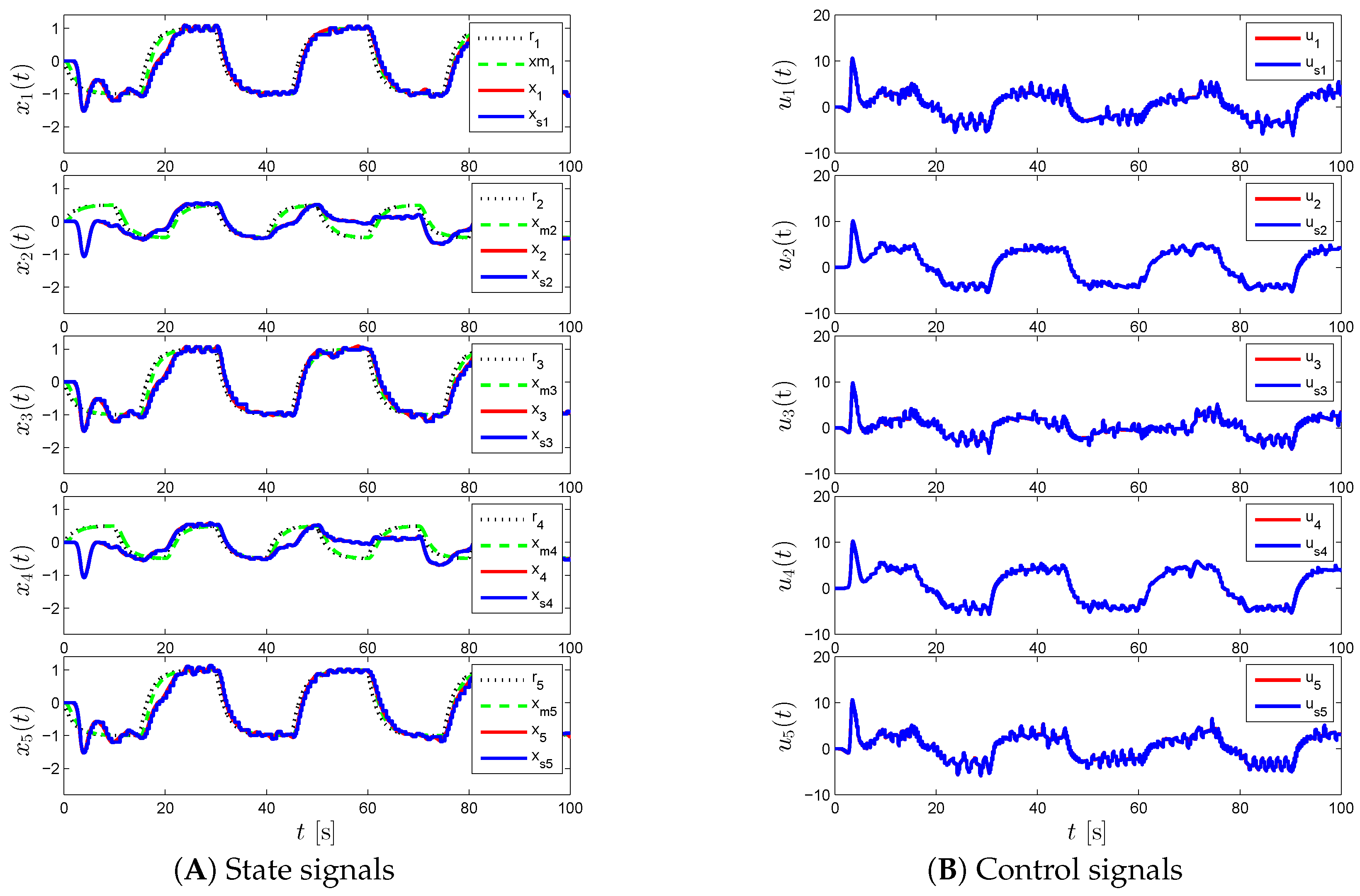
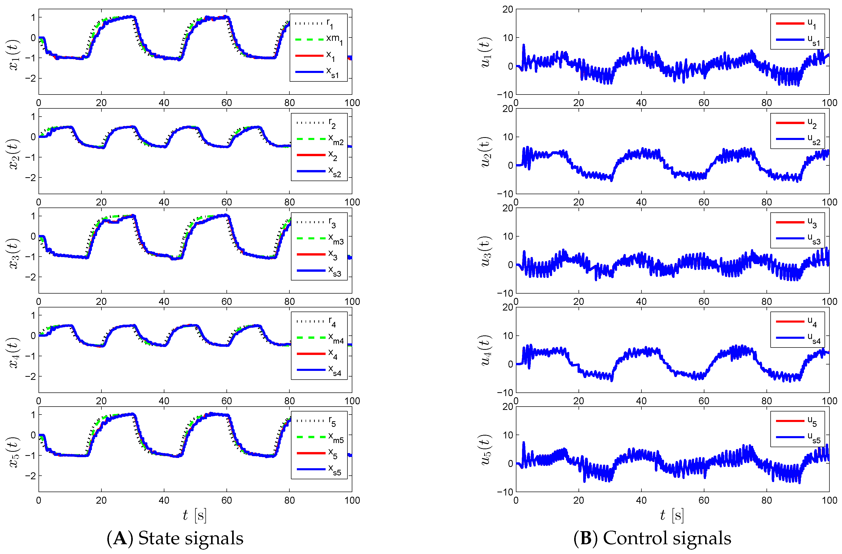
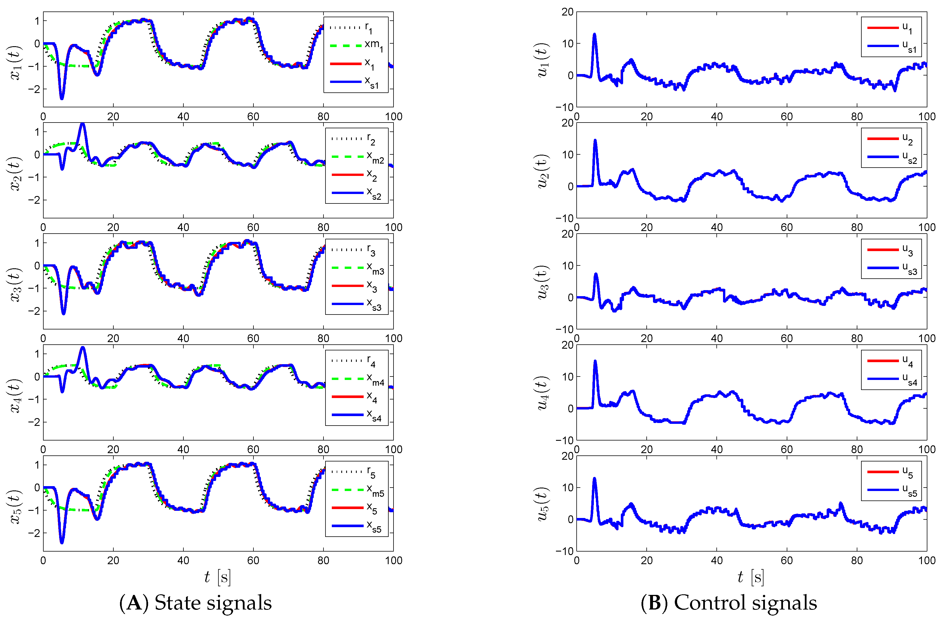
Theorem 1. 

Consider the uncertain large-scale modular system $\mathcal{S}$ consisting of N interconnected modules ${\mathcal{S}}_i$ described by Equation (14) subject to Assumptions 1–4. Consider, in addition, the reference model given by Equation (6), and the module feedback control law given by Equations (16) and (17). Moreover, let the data transmission from the uncertain dynamical module to the local controller occur when ${\overline{E}}_{1i}$ is true and the data transmission from the controller to the uncertain dynamical system occur when ${\overline{E}}_{2i}\vee E_{3i}$ is true. Then, the closed-loop solution $(e_i\left(t\right),{\tilde{W}}_i\left(t\right))$ is uniformly ultimately bounded for all $i=1,2,...,N$.

Proof. 

Since the data transmission from the uncertain modules to their local controllers and from the local controllers to the uncertain modules occur when ${\overline{E}}_{1i}$ and ${\overline{E}}_{2i}\vee E_{3i}$ are true, respectively, note that $∥x_{\mathrm{s}i}\left(t\right)-x_i\left(t\right)∥\le {ϵ}_{xi}$ and $∥u_{\mathrm{s}i}\left(t\right)-u_i\left(t\right)∥\le {ϵ}_{ui}$ hold. Consider now the Lyapunov-like function given by:

$$\begin{array}{c}\hfill {\mathcal{V}}_i(e_i,{\tilde{W}}_i)=e_i^{\mathrm{T}}{P}_i{e}_i+{\gamma }_i^{-1}\text{tr}\left({({\tilde{W}}_i{\mathrm{\Lambda }}_i^{\frac{1}{2}})}^{\mathrm{T}}(\widetilde{W_i}{\mathrm{\Lambda }}_i^{\frac{1}{2}})\right)\end{array}$$

(23)

Note that ${\mathcal{V}}_i(0,0)=0$ and ${\mathcal{V}}_i(e_i,{\tilde{W}}_i)>0$ for all $(e_i,{\tilde{W}}_i)\ne (0,0)$. The time-derivative of Equation (23) is given by:

$$\begin{array}{c}{\dot{\mathcal{V}}}_i(e_i\left(t\right),{\tilde{W}}_i\left(t\right))\hfill \\ =2e_i^{\mathrm{T}}\left(t\right)P{\dot{e}}_i\left(t\right)+2{\gamma }_i^{-1}\text{tr}\left({\tilde{W}}_i^{\mathrm{T}}\left(t\right){\dot{\tilde{W}}}_i\left(t\right){\mathrm{\Lambda }}_i\right)\hfill \\ \le 2e_i^{\mathrm{T}}\left(t\right)P_i(A_{\mathrm{r}i}{e}_i\left(t\right)-B_i{\mathrm{\Lambda }}_i{\tilde{W}}_i^{\mathrm{T}}\left(t\right){\sigma }_i\left(x_{\mathrm{s}i}\left(t\right),c_i\left(t\right)\right)-B_i{\mathrm{\Lambda }}_i{g}_i(·)+B_i\sum _{i\sim j}{\delta }_{ij}\left(x_j\left(t\right)\right)\hfill \\ +B_i{\mathrm{\Lambda }}_i(u_{\mathrm{s}i}\left(t\right)-u_i\left(t\right))+B_i{K}_{1i}(x_{\mathrm{s}i}\left(t\right)-x_i\left(t\right)))+2\text{tr}\left({\tilde{W}}_i^{\mathrm{T}}\left(t\right){\mathrm{\Lambda }}_i{\sigma }_i\left(x_{\mathrm{s}i}\left(t\right),c_i\left(t\right)\right)e_{\mathrm{s}i}^{\mathrm{T}}\left(t\right)P_i{B}_i\right)\hfill \\ \le -e_i^{\mathrm{T}}\left(t\right)R_i{e}_i\left(t\right)-2e_i^{\mathrm{T}}\left(t\right)P_i{B}_i{\mathrm{\Lambda }}_i{g}_i(·)+2e_i^{\mathrm{T}}\left(t\right)P_i{B}_i\sum _{i\sim j}{\delta }_{ij}\left(x_j\left(t\right)\right)+2e_i^{\mathrm{T}}\left(t\right)P_i{B}_i{\mathrm{\Lambda }}_i(u_{\mathrm{s}i}\left(t\right)-u_i\left(t\right))\hfill \\ +2e_i^{\mathrm{T}}\left(t\right)P_i{B}_i{K}_{1i}(x_{\mathrm{s}i}\left(t\right)-x_i\left(t\right))+2\text{tr}\left({\tilde{W}}_i^{\mathrm{T}}\left(t\right){\mathrm{\Lambda }}_i{\sigma }_i\left(x_{\mathrm{s}i}\left(t\right),c_i\left(t\right)\right){(x_{\mathrm{s}i}\left(t\right)-x_i\left(t\right))}^{\mathrm{T}}{P}_i{B}_i\right)\hfill \\ \le -{\lambda }_{\text{min}}\left(R_i\right)\parallel e_i\left(t\right){\parallel }^2+2\parallel e_i\left(t\right)\parallel {\lambda }_{\text{max}}\left(P_i\right)\parallel B_i{\parallel }_{\mathrm{F}}\parallel {\mathrm{\Lambda }}_i{\parallel }_{\mathrm{F}}\parallel g_i(·)\parallel +\parallel 2e_i\left(t\right)P_i{B}_i\sum _{i\sim j}{\delta }_{ij}\left(x_j\left(t\right)\right)\parallel \hfill \\ +2\parallel e_i\left(t\right)\parallel {\lambda }_{\text{max}}\left(P_i\right)\parallel B_i{\parallel }_{\mathrm{F}}\parallel {\mathrm{\Lambda }}_i{\parallel }_{\mathrm{F}}{ϵ}_{ui}+2\parallel e_i\left(t\right)\parallel {\lambda }_{\text{max}}\left(P_i\right)\parallel B_i{\parallel }_{\mathrm{F}}\parallel K_{1i}{\parallel }_{\mathrm{F}}{ϵ}_{xi}+2\parallel {\tilde{W}}_i\left(t\right){\parallel }_{\mathrm{F}}{\parallel {\mathrm{\Lambda }}_i\parallel }_{\mathrm{F}}\hfill \\ ·\parallel {\sigma }_i\left(x_{\mathrm{s}i}\left(t\right),c_i\left(t\right)\right)\parallel {ϵ}_{xi}{\lambda }_{\text{max}}\left(P_i\right){\parallel B_i\parallel }_{\mathrm{F}}\hfill \end{array}$$

(24)

It follows from Assumption 1 that an upper bound for $∥g_i(·)∥$ in Equation (24) can be given by:

$$\begin{array}{cc}\hfill ∥g_i(·)∥& =∥W_i^{\mathrm{T}}\left[{\sigma }_i\left(x_{\mathrm{s}i}\left(t\right),c_i\left(t\right)\right)-{\sigma }_i\left(x_i\left(t\right),x_{\mathrm{s}i}\left(t\right),c_i\left(t\right)\right)\right]∥\hfill \\ & \le \underset{K_{gi}}{\underbrace{\parallel {\mathrm{\Lambda }}_i^{-1}{\parallel }_{\mathrm{F}}{\omega }_i^{*}{L}_{\beta i}}}\parallel x_{\mathrm{s}i}\left(t\right)-x_i\left(t\right)\parallel \le K_{gi}{ϵ}_{xi}\hfill \end{array}$$

(25)

where $K_{gi}\in {\mathbb{R}}_{+}$. In addition, one can compute an upper bound for $\parallel {\sigma }_i\left(x_{\mathrm{s}i}\left(t\right),c_i\left(t\right)\right)\parallel$ in Equation (24) as:

$$\begin{array}{cc}\hfill \parallel {\sigma }_i\left(x_{\mathrm{s}i}\left(t\right),c_i\left(t\right)\right)\parallel & \le \parallel {\beta }_i\left(x_{\mathrm{s}i}\left(t\right)\right)\parallel +\parallel x_{\mathrm{s}i}\left(t\right)\parallel +\parallel c_i\left(t\right)\parallel \hfill \\ & \le L_{\beta i}\parallel x_{\mathrm{s}i}\left(t\right)\parallel +\parallel x_{\mathrm{s}i}\left(t\right)\parallel +\parallel c_i\left(t\right)\parallel \hfill \\ & =(L_{\beta i}+1){ϵ}_{xi}+(L_{\beta i}+1)\parallel e_i\left(t\right)\parallel +(L_{\beta i}+1)x_{\mathrm{r}i}^{*}+\parallel c_i\left(t\right)\parallel \hfill \end{array}$$

(26)

where $\parallel x_{\mathrm{r}i}\left(t\right)\parallel \le x_{\mathrm{r}i}^{*}$. Then, using the bounds given by Equations (25) and (26) in Equation (24), one can write:

$$\begin{array}{c}{\dot{\mathcal{V}}}_i(e_i\left(t\right),{\tilde{W}}_i\left(t\right))\hfill \\ \le -{\lambda }_{\text{min}}\left(R_i\right)\parallel e_i\left(t\right){\parallel }^2+(2{\lambda }_{\text{max}}\left(P_i\right)\parallel B_i{\parallel }_{\mathrm{F}}\parallel {\mathrm{\Lambda }}_i{\parallel }_{\mathrm{F}}{K}_{gi}{ϵ}_{xi}+2{\lambda }_{\text{max}}\left(P_i\right)\parallel B_i{\parallel }_{\mathrm{F}}{\parallel {\mathrm{\Lambda }}_i\parallel }_{\mathrm{F}}{ϵ}_{ui}+2{\lambda }_{\text{max}}\left(P_i\right)\hfill \\ ·\parallel B_i{\parallel }_{\mathrm{F}}\parallel K_{1i}{\parallel }_{\mathrm{F}}{ϵ}_{xi}+2\parallel {\tilde{W}}_i{\left(t\right)\parallel }_{\mathrm{F}}\parallel {\mathrm{\Lambda }}_i{\parallel }_{\mathrm{F}}(L_{\beta i}+1){\lambda }_{\text{max}}\left(P_i\right)\parallel B_i{\parallel }_{\mathrm{F}}{ϵ}_{xi})\parallel e_i\left(t\right)\parallel +2\parallel {\tilde{W}}_i\left(t\right){\parallel }_{\mathrm{F}}{\parallel {\mathrm{\Lambda }}_i\parallel }_{\mathrm{F}}\hfill \\ ·\left((L_{\beta i}+1){ϵ}_{xi}+(L_{\beta i}+1)x_{\mathrm{r}i}^{*}+\parallel c_i\left(t\right)\parallel \right){\lambda }_{\text{max}}\left(P_i\right)\parallel B_i{\parallel }_{\mathrm{F}}{ϵ}_{xi}+\parallel 2e_i\left(t\right)P_i{B}_i\sum _{i\sim j}{\delta }_{ij}\left(x_j\left(t\right)\right)\parallel \hfill \\ =-c_{1i}\parallel e_i{\left(t\right)\parallel }^2+c_{2i}\parallel e_i\left(t\right)\parallel +c_{3i}+\parallel 2e_i\left(t\right)P_i{B}_i{\delta }_{ij}\left(x_j\left(t\right)\right)\parallel \hfill \end{array}$$

(27)

where $c_{1i}\triangleq {\lambda }_{\text{min}}\left(R_i\right)$, $c_{2i}\triangleq 2{\lambda }_{\text{max}}\left(P_i\right)\parallel B_i{\parallel }_{\mathrm{F}}\parallel {\mathrm{\Lambda }}_i{\parallel }_{\mathrm{F}}{K}_{gi}{ϵ}_{xi}+2{\lambda }_{\text{max}}\left(P_i\right)\parallel B_i{\parallel }_{\mathrm{F}}\parallel {\mathrm{\Lambda }}_i{\parallel }_{\mathrm{F}}{ϵ}_{ui}+2{\lambda }_{\text{max}}\left(P_i\right)\parallel B_i{\parallel }_{\mathrm{F}}{\parallel K_{1i}\parallel }_{\mathrm{F}}·{ϵ}_{xi}$ + 2${\tilde{w}}_i^{*}\parallel {\mathrm{\Lambda }}_i{\parallel }_{\mathrm{F}}(L_{\beta i}+1){\lambda }_{\text{max}}\left(P_i\right){\parallel B_i\parallel }_{\mathrm{F}}{ϵ}_{xi}$ and $c_{3i}\triangleq 2{\tilde{w}}_i^{*}\parallel {\mathrm{\Lambda }}_i{\parallel }_{\mathrm{F}}\left((L_{\beta i}+1){ϵ}_{xi}+(L_{\beta i}+1)x_{\mathrm{r}i}^{*}+\parallel c_i\left(t\right)\parallel \right){\lambda }_{\text{max}}\left(P_i\right){\parallel B_i\parallel }_{\mathrm{F}}{ϵ}_{xi}$ with $\left|\right|{\tilde{W}}_i\left(t\right){\left|\right|}_{\mathrm{F}}\le {\tilde{w}}_i^{*}$ due to utilizing the projection operator in the weight update law given by Equation (9).

Since $x_j\left(t\right)=e_j\left(t\right)+x_{\mathrm{r}j}\left(t\right)$ with $\parallel x_{\mathrm{r}j}\left(t\right)\parallel \le x_{\mathrm{r}j}^{*}$, it follows from Assumption 2 that:

$$\begin{array}{c}\hfill \parallel \sum _{i\sim j}{\delta }_{ij}\left(x_j\left(t\right)\right)\parallel \le \sum _{i\sim j}{\alpha }_{ij}\left[\parallel e_j\left(t\right)\parallel +x_{\mathrm{r}j}^{*}\right]\end{array}$$

(28)

Furthermore, using Equation (28) in the last term of Equation (27) results in:

$$\begin{array}{cc}\hfill \parallel 2e_i\left(t\right)P_i{B}_i{\delta }_{ij}\left(x_j\left(t\right)\right)\parallel & \le 2{\lambda }_{\text{max}}\left(P_i\right)\parallel e_i\left(t\right)\parallel \parallel B_i{\parallel }_{\mathrm{F}}\parallel \sum _{i\sim j}{\delta }_{ij}\left(x_j\left(t\right)\right)\parallel \hfill \\ & \le 2{\lambda }_{\text{max}}\left(P_i\right)\parallel e_i\left(t\right)\parallel \parallel B_i{\parallel }_{\mathrm{F}}\sum _{i\sim j}{\alpha }_{ij}\left[\parallel e_j\left(t\right)\parallel +x_{\mathrm{r}j}^{*}\right]\hfill \\ & \le {\lambda }_{\text{max}}\left(P_i\right){\parallel B_i\parallel }_{\mathrm{F}}\sum _{i\sim j}{\alpha }_{ij}\left[2\parallel e_i\left(t\right)\parallel \parallel e_j\left(t\right)\parallel +2\parallel e_i\left(t\right)\parallel x_{\mathrm{r}j}^{*}\right]\hfill \\ & \le {\lambda }_{\text{max}}\left(P_i\right){\parallel B_i\parallel }_{\mathrm{F}}\sum _{i\sim j}{\alpha }_{ij}\left[2\parallel e_i{\left(t\right)\parallel }^2+{\parallel e_j\left(t\right)\parallel }^2+{x_{\mathrm{r}j}^{*}}^2\right]\hfill \end{array}$$

(29)

where Young’s inequality [46] is considered in the scalar form of $2xy\le \nu x^2+y^2/\nu$, where $x,y\in \mathbb{R}$ and $\nu >0$, and applied to terms $\parallel e_i\left(t\right)\parallel \parallel e_j\left(t\right)\parallel$ and $\parallel e_i\left(t\right)\parallel x_{\mathrm{r}j}^{*}$ with $\nu =1$. Hence, Equation (27) becomes:

$$\begin{array}{cc}\hfill {\dot{\mathcal{V}}}_i(e_i\left(t\right),{\tilde{W}}_i\left(t\right))& \le -\underset{d_{1i}}{\underbrace{\left[c_{1i}-2{\lambda }_{\text{max}}\left(P_i\right){\parallel B_i\parallel }_{\mathrm{F}}\sum _{i\sim j}{\alpha }_{ij}\right]}}\parallel e_i{\left(t\right)\parallel }^2+\underset{f_i}{\underbrace{{\lambda }_{\text{max}}\left(P_i\right){\parallel B_i\parallel }_{\mathrm{F}}}}\sum _{i\sim j}{\alpha }_{ij}{\parallel e_j\left(t\right)\parallel }^2\hfill \\ & +c_{2i}\parallel e_i\left(t\right)\parallel +{\phi }_i\hfill \end{array}$$

(30)

where ${\phi }_i\triangleq c_{3i}+{\lambda }_{\text{max}}\left(P_i\right){\parallel B_i\parallel }_{\mathrm{F}}{\sum }_{i\sim j}{\alpha }_{ij}{x_{\mathrm{r}j}^{*}}^2$.

Introducing:

$$\begin{array}{c}\hfill \mathcal{V}(·)=\sum _{i=1}^N{\mathcal{V}}_i(e_i\left(t\right),{\tilde{W}}_i\left(t\right))\end{array}$$

(31)

for the uncertain system $\mathcal{S}$ results in:

$$\begin{array}{cc}\hfill \dot{\mathcal{V}}(·)& \le \sum _{i=1}^N[-d_{1i}\parallel e_i{\left(t\right)\parallel }^2+f_i\sum _{i\sim j}{\alpha }_{ij}\parallel e_j{\left(t\right)\parallel }^2+c_{2i}\parallel e_i\left(t\right)\parallel +{\phi }_i]\hfill \\ & =\sum _{i=1}^N[-\underset{D_{1i}}{\underbrace{\left(d_{1i}-\sum _{i\sim j}{f}_j{\alpha }_{ji}\right)}}\parallel e_i{\left(t\right)\parallel }^2+c_{2i}\parallel e_i\left(t\right)\parallel +{\phi }_i]\hfill \end{array}$$

(32)

where $D_{1i}>0$ is defined in Assumption 4. Letting $e_a\left(t\right)\triangleq {\left[\parallel e_1\left(t\right)\parallel ,\cdots ,\parallel e_N\left(t\right)\parallel \right]}^{\mathrm{T}}$, $D_1\triangleq \text{diag}\left(\right[D_{11},\cdots ,D_{1N}\left]\right)$, $C_2\triangleq \text{diag}\left(\left[c_{21},\cdots ,c_{2N}\right]\right)$ and ${\phi }_a\triangleq {\sum }_{i=1}^N{\phi }_i$, Equation (32) can equivalently be written as:

$$\begin{array}{cc}\hfill \dot{\mathcal{V}}(·)& \le -e_a^{\mathrm{T}}\left(t\right)D_1{e}_a\left(t\right)+C_2{e}_a\left(t\right)+{\phi }_a\hfill \\ & \le -{\lambda }_{\text{min}}\left(D_1\right)\parallel e_a\left(t\right){\parallel }^2+{\lambda }_{\text{max}}\left(C_2\right)\parallel e_a\left(t\right)\parallel +{\phi }_a\hfill \end{array}$$

(33)

When $\parallel e_a\left(t\right)\parallel >\psi$, this renders $\dot{\mathcal{V}}(·)<0$, where $\psi \triangleq \frac{\frac{{\lambda }_{\text{max}}\left(C_2\right)}{2\sqrt{{\lambda }_{\text{min}}\left(D_1\right)}}+\sqrt{\frac{{\lambda }_{\text{max}}^2\left(C_2\right)}{4{\lambda }_{\text{min}}\left(D_1\right)}+{\phi }_a}}{\sqrt{{\lambda }_{\text{min}}\left(D_1\right)}}$. Hence, $e_i\left(t\right)$ and ${\tilde{W}}_i\left(t\right)$ are uniformly ultimate bounded for all $i=1,2,...,N$. ☐

2.2.2. Computation of the Ultimate Bound for System Performance Assessment

For revealing the effect of user-defined thresholds and the event-triggered feedback adaptive controller design parameters to the system performance, the next corollary presents a computation of the ultimate bound for the system $\mathcal{S}$. For this purpose, we define the following, $P_{min}\triangleq \text{diag}\left(\left[{\lambda }_{min}\left(P_1\right),\cdots ,{\lambda }_{min}\left(P_N\right)\right]\right)$, $P_{max}\triangleq \text{diag}\left(\left[{\lambda }_{max}\left(P_1\right),\cdots ,{\lambda }_{max}\left(P_N\right)\right]\right)$, ${\gamma }_a\triangleq \text{diag}\left(\left[{\gamma }_1^{-1},\cdots ,{\gamma }_N^{-1}\right]\right)$, ${\mathrm{\Lambda }}_a\triangleq \text{diag}\left(\left[\parallel {\mathrm{\Lambda }}_1{\parallel }_{\mathrm{F}},\cdots ,{\parallel {\mathrm{\Lambda }}_N\parallel }_{\mathrm{F}}\right]\right)$, ${\tilde{W}}_a\left(t\right)\triangleq {\left[\parallel {\tilde{W}}_1{\left(t\right)\parallel }_{\mathrm{F}},\cdots ,{\parallel {\tilde{W}}_N\left(t\right)\parallel }_{\mathrm{F}}\right]}^{\mathrm{T}}$.

Corollary 1. 

Consider the uncertain dynamical system $\mathcal{S}$ consisting of N interconnected modules ${\mathcal{S}}_i$ described by Equation (14) subject to Assumptions 1–4. Consider, in addition, the reference model given by Equation (6), and the module feedback control law given by Equations (16) and (17). Moreover, let the data transmission from the uncertain modules to their local controllers occur when ${\overline{E}}_{1i}$ is true and the data transmission from the controllers to the uncertain modules occur when ${\overline{E}}_{2i}\vee E_{3i}$ is true. Then, the ultimate bound of the system error between the uncertain dynamical system and the reference model is given by:

$$\begin{array}{c}\hfill \left|\right|e_a\left(t\right)\left|\right|\le \tilde{\mathrm{\Phi }}{\lambda }_{min}^{-\frac{1}{2}}\left(P_{min}\right),t\ge T\end{array}$$

(34)

where:

$$\begin{array}{c}\hfill \tilde{\mathrm{\Phi }}\triangleq {[{\lambda }_{max}\left(P_{max}\right){\psi }^2+{\lambda }_{max}\left({\gamma }_a\right){\lambda }_{max}\left({\mathrm{\Lambda }}_a\right){\parallel {\tilde{W}}_a\left(t\right)\parallel }^2]}^{\frac{1}{2}}\end{array}$$

(35)

Proof. 

It follows from the proof of Theorem 1 that $\dot{\mathcal{V}}(e_a\left(t\right),{\tilde{W}}_a\left(t\right))\le 0$ outside the compact set given by:

$$\begin{array}{c}\hfill \mathcal{S}\triangleq \left\{e_a\left(t\right):∥e_a\left(t\right)∥\le \psi \right\}\end{array}$$

(36)

That is, since $\mathcal{V}(e_a\left(t\right),{\tilde{W}}_a\left(t\right))$ cannot grow outside $\mathcal{S}$, the evolution of $\mathcal{V}(e_a\left(t\right),{\tilde{W}}_a\left(t\right))$ is upper bounded by:

$$\begin{array}{ccc}\hfill \mathcal{V}(e_a\left(t\right),{\tilde{W}}_a\left(t\right))& \le & \underset{e_a\left(t\right)\in \mathcal{S}}{max}\mathcal{V}(e_a\left(t\right),{\tilde{W}}_a\left(t\right))\hfill \\ & =& {\lambda }_{max}\left(P_{max}\right){\psi }^2+{\lambda }_{max}\left({\gamma }_a\right){\lambda }_{max}\left({\mathrm{\Lambda }}_a\right){\parallel {\tilde{W}}_a\left(t\right)\parallel }^2\hfill \\ & =& {\tilde{\mathrm{\Phi }}}^2\hfill \end{array}$$

(37)

It follows from $e_a^{\mathrm{T}}{P}_{min}{e}_a\le \mathcal{V}(e_a,{\tilde{W}}_a)$ that ${∥e_a\left(t\right)∥}^2\le \frac{{\tilde{\mathrm{\Phi }}}^2}{{\lambda }_{min}\left(P_{min}\right)}$, and Equation (34) is immediate. ☐

2.2.3. Computation of the Event-Triggered Inter-Sample Time Lower Bound

We now show that the proposed event-triggered decentralized adaptive control architecture does not yield to a Zeno behavior, which implies that it does not require a continuous two-way data exchange and reduces wireless network utilization. For the following corollary presenting the result of this subsection, we consider $r_{q_i}^{k_i}\in \left(s_{k_i},s_{k_i+1}\right)$ to be the ${\mathit{q}}_i$-th time instant when $E_{2i}$ is violated over $\left(s_{k_i},s_{k_i+1}\right)$, and since ${\left\{s_{k_i}\right\}}_{k_i=1}^{\infty }$ is a subsequence of ${\left\{r_{j_i}\right\}}_{j_i=1}^{\infty }$, it follows that ${\left\{r_{j_i}\right\}}_{j_i=1}^{\infty }={\left\{s_{k_i}\right\}}_{k_i=1}^{\infty }\bigcup {\left\{r_{q_i}^{k_i}\right\}}_{k_i=1,q_i=1}^{\infty ,m_{k_i}}$, where $m_{k_i}\in \mathbb{N}$ is the number of violation times of $E_{2i}$ over $\left(s_{k_i},s_{k_i+1}\right)$.

Corollary 2. 

Consider the uncertain dynamical system $\mathcal{S}$ consisting of N interconnected modules ${\mathcal{S}}_i$ described by Equation (14) subject to Assumptions 1–4. Consider, in addition, the reference model given by Equation (6), and the module feedback control law given by Equations (16) and (17). Moreover, let the data transmission from the uncertain dynamical module to the local controller occur when ${\overline{E}}_{1i}$ is true and the data transmission from the controller to the uncertain dynamical system occur when ${\overline{E}}_{2i}\vee E_{3i}$ is true. Then, there exist positive scalars ${\alpha }_{xi}\triangleq \frac{{ϵ}_{xi}}{{\mathrm{\Phi }}_{1i}}$ and ${\alpha }_{ui}\triangleq \frac{{ϵ}_{ui}}{{\mathrm{\Phi }}_{2i}}$ such that:

$$\begin{array}{ccc}\hfill s_{k_i+1}-s_{k_i}& >& {\alpha }_{xi},\forall k_i\in \mathbb{N}\hfill \end{array}$$

(38)

$$\begin{array}{ccc}\hfill r_{q_i+1}^{k_i}-r_{q_i}^{k_i}& >& {\alpha }_{ui},\forall q_i\in \left\{0,...,m_{k_i}\right\},\forall k_i\in \mathbb{N}\hfill \end{array}$$

(39)

Proof. 

The time derivative of $∥x_{\mathrm{s}i}\left(t\right)-x_i\left(t\right)∥$ over $t\in \left(s_{k_i},s_{k_i+1}\right)$, $\forall k_i\in \mathbb{N}$, is given by:

$$\begin{array}{ccc}\hfill {\displaystyle \frac{d}{dt}}∥x_{\mathrm{s}i}\left(t\right)-x_i\left(t\right)∥& \le & ∥{\dot{x}}_{\mathrm{s}i}\left(t\right)-{\dot{x}}_i\left(t\right)∥=∥{\dot{x}}_i\left(t\right)∥\hfill \\ & \le & \parallel A_{\mathrm{r}i}{\parallel }_{\mathrm{F}}\left[\parallel e_i\left(t\right)\parallel +x_{\mathrm{r}i}^{*}\right]+\parallel B_{\mathrm{r}i}{\parallel }_{\mathrm{F}}\parallel c_i\left(t\right)\parallel +\parallel B_i{\parallel }_{\mathrm{F}}\parallel {\mathrm{\Lambda }}_i{\parallel }_{\mathrm{F}}{\tilde{w}}_i^{*}\left[L_{\beta i}\right({ϵ}_{xi}+\parallel e_i\left(t\right)\parallel \hfill \\ & & +x_{\mathrm{r}i}^{*})+\parallel K_{1i}{\parallel }_{\mathrm{F}}\left({ϵ}_{xi}+\parallel e_i\left(t\right)\parallel +x_{\mathrm{r}i}^{*}\right)+\parallel K_{2i}{\parallel }_{\mathrm{F}}\parallel c_i\left(t\right)\parallel ]+\parallel B_i{\parallel }_{\mathrm{F}}{\parallel {\mathrm{\Lambda }}_i\parallel }_{\mathrm{F}}{K}_{gi}{ϵ}_{xi}\hfill \\ & & +\parallel B_i{\parallel }_{\mathrm{F}}\sum _{i\sim j}{\alpha }_{ij}\left(\parallel e_j\left(t\right)\parallel +x_{\mathrm{r}j}^{*}\right)+\parallel B_i{\parallel }_{\mathrm{F}}\parallel {\mathrm{\Lambda }}_i{\parallel }_{\mathrm{F}}{ϵ}_{ui}+\parallel B_i{\parallel }_{\mathrm{F}}{\parallel K_{1i}\parallel }_{\mathrm{F}}{ϵ}_{xi}\hfill \end{array}$$

(40)

Since the closed-loop dynamical system is uniformly ultimately bounded by Theorem 1, there exists an upper bound to Equation (40). Letting ${\mathrm{\Phi }}_{1i}$ denote this upper bound and with the initial condition satisfying ${lim}_{t\to s_{k_i}^{+}}\parallel x_{\mathrm{s}i}\left(t\right)-x_i\left(t\right)\parallel =0$, it follows from Equation (40) that:

$$\begin{array}{c}\hfill \parallel x_{\mathrm{s}i}\left(t\right)-x_i\left(t\right)\parallel \le {\mathrm{\Phi }}_{1i}(t-s_{k_i}),\forall t\in (s_{k_i},s_{k_i+1})\end{array}$$

(41)

Therefore, when ${\overline{E}}_{1i}$ is true, then ${lim}_{t\to s_{k_i+1}^{-}}\parallel x_{\mathrm{s}i}\left(t\right)-x_i\left(t\right)\parallel ={ϵ}_{xi}$, and it then follows from Equation (41) that $s_{k_i+1}-s_{k_i}\ge {\alpha }_{xi}$.

Similarly, the time derivative of $∥u_{\mathrm{s}i}\left(t\right)-u_i\left(t\right)∥$ over $t\in \left(r_{q_i}^{k_i},r_{q_i+1}^{k_i}\right),\forall q_i\in \mathbb{N}$, is given by:

$$\begin{array}{ccc}\hfill {\displaystyle \frac{d}{dt}}∥u_{\mathrm{s}i}\left(t\right)-u_i\left(t\right)∥& \le & ∥{\dot{u}}_{\mathrm{s}i}\left(t\right)-{\dot{u}}_i\left(t\right)∥=∥{\dot{u}}_i\left(t\right)∥\hfill \\ & =& ∥{\dot{\widehat{W}}}_i^{\mathrm{T}}\left(t\right){\sigma }_i\left(x_{\mathrm{s}i}\left(t\right),c_i\left(t\right)\right)+{\widehat{W}}_i^{\mathrm{T}}\left(t\right){\dot{\sigma }}_i\left(x_{\mathrm{s}i}\left(t\right),c_i\left(t\right)\right)∥\hfill \\ & \le & {\gamma }_i{∥B_i∥}_{\mathrm{F}}{\lambda }_{\text{max}}\left(P_i\right)∥e_{\mathrm{s}i}\left(t\right)∥{∥{\sigma }_i\left(x_{\mathrm{s}i}\left(t\right),c_i\left(t\right)\right)∥}^2+\parallel {\mathrm{\Lambda }}_i^{-1}{\parallel }_{\mathrm{F}}\parallel K_{2i}{\parallel }_{\mathrm{F}}\parallel {\dot{c}}_i\left(t\right)\parallel \hfill \\ & \le & {\gamma }_i{∥B_i∥}_{\mathrm{F}}{\lambda }_{\text{max}}\left(P_i\right)\left(∥e_i\left(t\right)∥+{ϵ}_{xi}\right)[L_{\beta i}({ϵ}_{xi}+∥e_i\left(t\right)∥+x_{\mathrm{r}i}^{*})+\parallel K_{1i}{\parallel }_{\mathrm{F}}({ϵ}_{xi}\hfill \\ & & +∥e_i\left(t\right)∥+x_{\mathrm{r}i}^{*})+\parallel K_{2i}{\parallel }_{\mathrm{F}}\parallel c_i\left(t\right)\parallel {]}^2+\parallel {\mathrm{\Lambda }}_i^{-1}{\parallel }_{\mathrm{F}}\parallel K_{2i}{\parallel }_{\mathrm{F}}\parallel {\dot{c}}_i\left(t\right)\parallel \hfill \end{array}$$

(42)

Once again, since the closed-loop dynamical system is uniformly ultimately bounded by Theorem 1, there exists an upper bound to Equation (42). Letting ${\mathrm{\Phi }}_{2i}$ denote this upper bound, and with the initial condition satisfying ${lim}_{t\to r_{q_i}^{k_{i+}}}∥u_{\mathrm{s}i}\left(t\right)-u_i\left(t\right)∥=0$, it follows from Equation (42) that:

$$\begin{array}{c}\hfill ∥u_{\mathrm{s}i}\left(t\right)-u_i\left(t\right)∥\le {\mathrm{\Phi }}_{2i}(t-r_{q_i}^{k_i}),\forall t\in \left(r_{q_i}^{k_i},r_{q_i+1}^{k_i}\right)\end{array}$$

(43)

Therefore, when ${\overline{E}}_{2i}\vee E_{3i}$ is true, then ${lim}_{t\to r_{q_i+1}^{k_{i-}}}∥u_{\mathrm{s}i}\left(t\right)-u_i\left(t\right)∥={ϵ}_{ui}$, and it then follows from Equation (43) that $r_{q_i+1}^{k_i}-r_{q_i}^{k_i}\ge {\alpha }_{ui}$. ☐

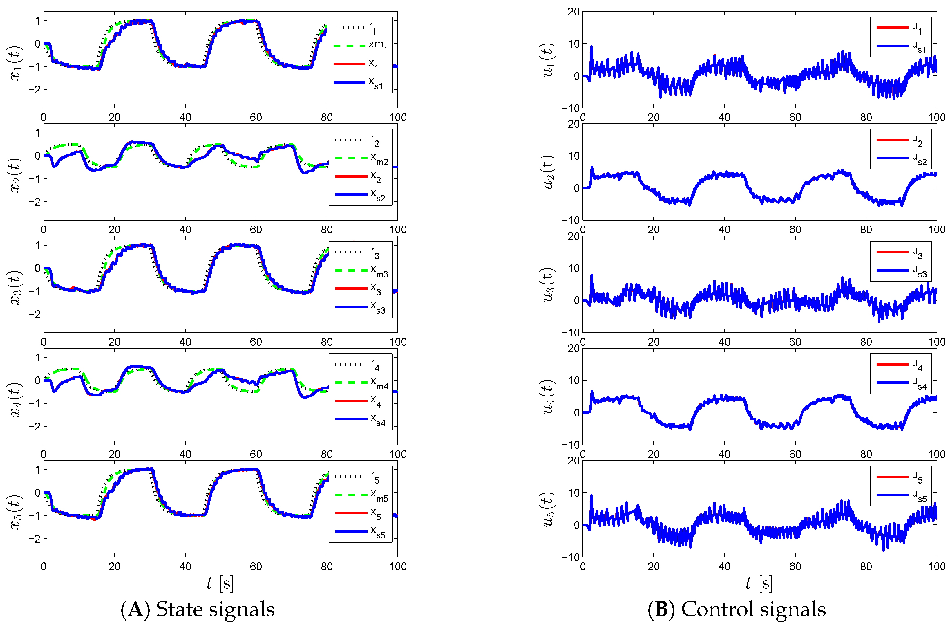
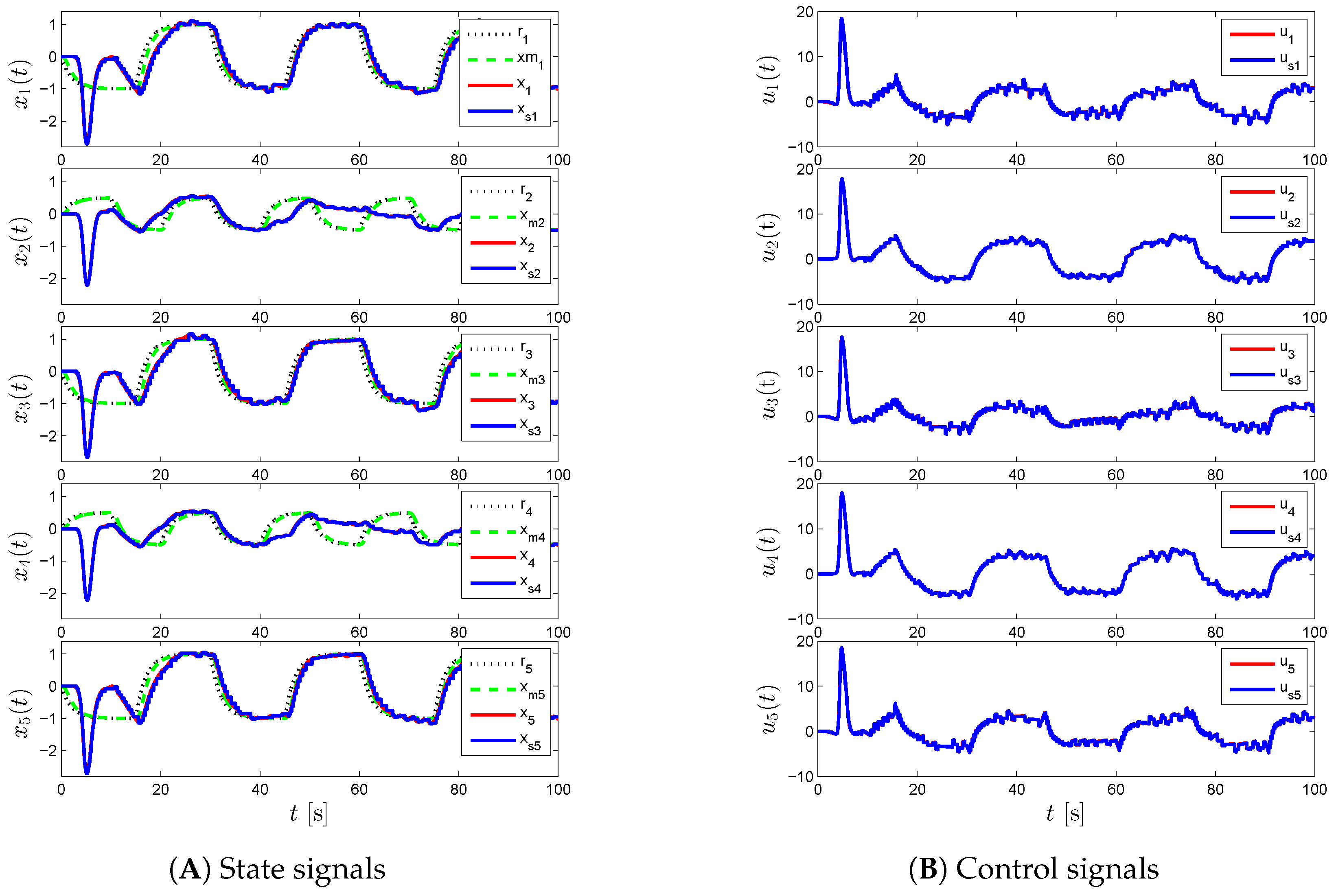
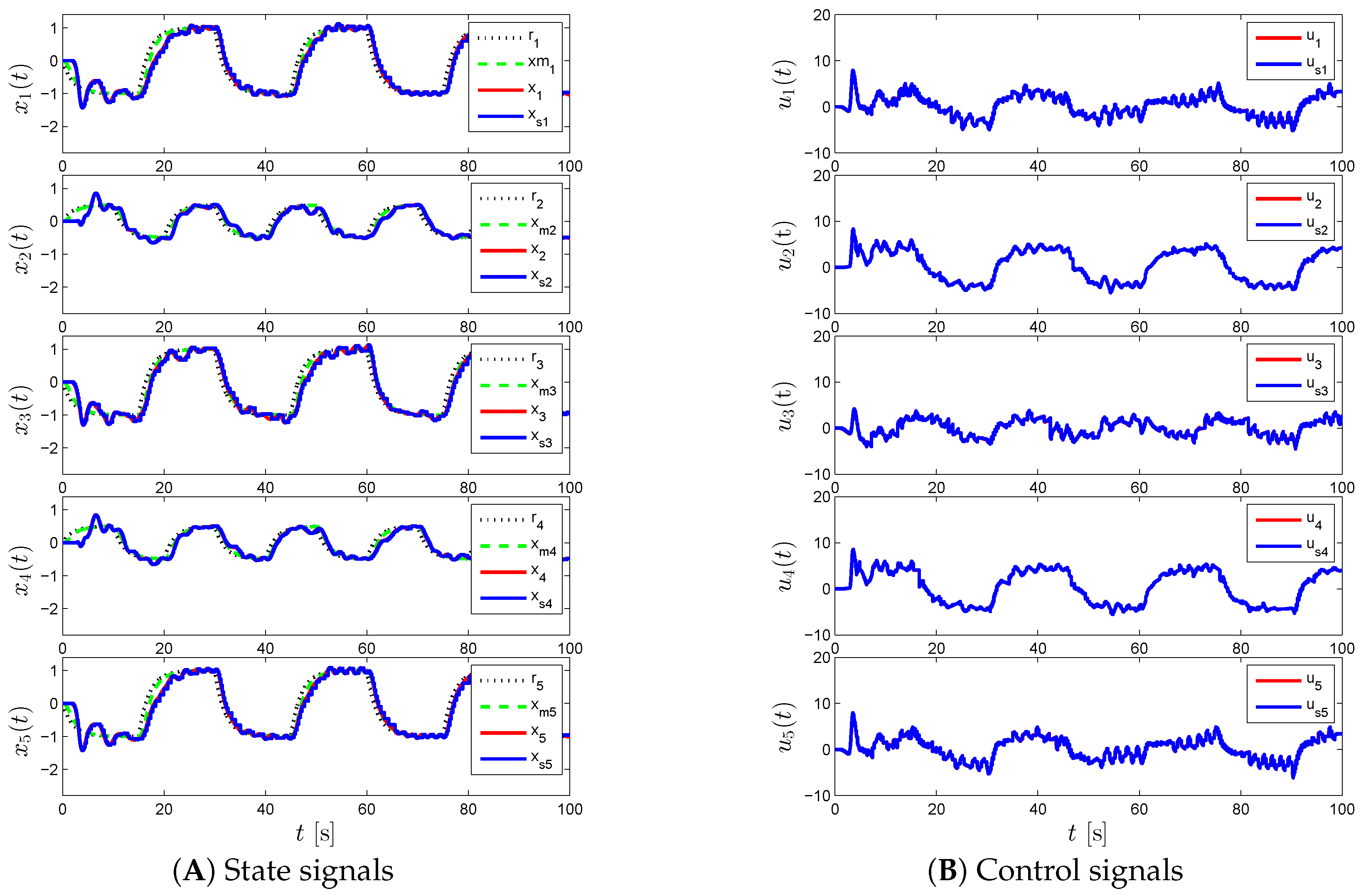
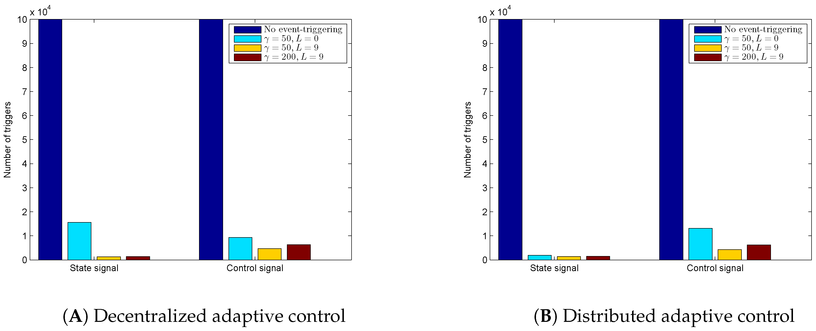
Corollary 2 shows that the inter-sample times for the module state vector and decentralized feedback control vector are bounded away from zero, and hence, the proposed event-triggered adaptive control approach does not yield to a Zeno behavior. As discussed earlier, this implies that the proposed event-triggered decentralized adaptive control methodology does not require a continuous two-way data exchange, and it reduces wireless network utilization.

2.2.4. Generalizations to the Event-Triggered Decentralized Adaptive Control with State Emulator

We now generalize our framework to a state emulator-based design, since this framework has the capability to suppress possible high-frequency oscillation in the control signal of the uncertain module ${\mathcal{S}}_i$ [10,13,37,38,39,40,41,42]. Consider the (modified) reference system, so-called the state emulator of ${\mathcal{S}}_i$, given by:

$$\begin{array}{c}\hfill {\dot{\widehat{x}}}_i\left(t\right)=A_{\mathrm{r}i}{\widehat{x}}_i\left(t\right)+B_{\mathrm{r}i}{c}_i\left(t\right)+L_i\left(x_{\mathrm{s}i}\left(t\right)-{\widehat{x}}_i\left(t\right)\right),{\widehat{x}}_i\left(0\right)={\widehat{x}}_{i0}\end{array}$$

(44)

where $L_i\in {\mathbb{R}}_{+}^{n_i\times n_i}\cap {\mathbb{D}}^{n_i\times n_i}$ is the state emulator gain. Letting ${\widehat{e}}_i\left(t\right)\triangleq {\widehat{x}}_i\left(t\right)-x_{\mathrm{r}i}\left(t\right)\in {\mathbb{R}}^{n_i}$, the reference model error dynamics capturing the difference between the ideal reference model in Equation (6) and the state emulator-based (modified) reference model in Equation (44) is given by:

$$\begin{array}{c}\hfill {\dot{\widehat{e}}}_i\left(t\right)=A_{\mathrm{r}i}{\widehat{e}}_i\left(t\right)+L_i\left(x_{\mathrm{s}i}\left(t\right)-{\widehat{x}}_i\left(t\right)\right)\end{array}$$

(45)

In addition, letting ${\tilde{x}}_i\left(t\right)\triangleq x_i\left(t\right)-{\widehat{x}}_i\left(t\right)\in {\mathbb{R}}^{n_i}$ to denote the system state error vector, the (state emulator-based) system error dynamics follows from Equations (18) and (44) as:

$$\begin{array}{ccc}\hfill {\dot{\tilde{x}}}_i\left(t\right)& =& A_{Li}{\tilde{x}}_i\left(t\right)-B_i{\mathrm{\Lambda }}_i{\tilde{W}}_i^{\mathrm{T}}\left(t\right){\sigma }_i\left(x_{\mathrm{s}i}\left(t\right),c_i\left(t\right)\right)-B_i{\mathrm{\Lambda }}_i{g}_i(·)+B_i{\delta }_{ij}\left(x_j\left(t\right)\right)+B_i{\mathrm{\Lambda }}_i(u_{\mathrm{s}i}\left(t\right)-u_i\left(t\right))\hfill \\ & & +(B_i{K}_{1i}-L_i)(x_{\mathrm{s}i}\left(t\right)-x_i\left(t\right)),{\tilde{x}}_i\left(0\right)={\tilde{x}}_{i0}\hfill \end{array}$$

(46)

where $A_{Li}\triangleq A_{\mathrm{r}i}-L_i\in {\mathbb{R}}^{n_i\times n_i}$ is Hurwitz by a suitable selection of the state emulator gain $L_i$ (e.g., $A_{Li}$ is Hurwitz with $L_i={\kappa }_{i}I$, ${\kappa }_i\in {\mathbb{R}}_{+}$, since $A_{\mathrm{r}i}$ is Hurwitz). To maintain system stability, we utilize the adaptive controller given by Equation (16) with the update law described by:

$$\begin{array}{c}\hfill {\dot{\widehat{W}}}_i\left(t\right)\triangleq {\gamma }_i{\mathrm{Proj}}_{\mathrm{m}}[{\widehat{W}}_i\left(t\right),{\sigma }_i\left(x_{\mathrm{s}i}\left(t\right),c_i\left(t\right)\right){(x_{\mathrm{s}i}\left(t\right)-{\widehat{x}}_i\left(t\right))}^{\mathrm{T}}{P}_i{B}_i],{\widehat{W}}_i\left(0\right)={\widehat{W}}_{i0}\end{array}$$

(47)

where $P_i\in {\mathbb{R}}_{+}^{n_i\times n_i\cap {\mathbb{S}}^{n_i\times n_i}}$ is the unique solution of the algebraic Riccati equation:

$$\begin{array}{c}\hfill 0=A_{Li}^{\mathrm{T}}{P}_i+P_i{A}_{Li}-P_i{B}_i{R}_i^{-1}{B}_i^{\mathrm{T}}{P}_i+Q_i\end{array}$$

(48)

with $R_i\in {\mathbb{R}}_{+}^{m_i\times m_i}\cap {\mathbb{S}}^{n_i\times n_i}$ and $Q_i\in {\mathbb{R}}_{+}^{n_i\times n_i}\cap {\mathbb{S}}^{n_i\times n_i}$.

Note from [10,42] that the state emulator-based adaptive control framework achieves stringent transient and steady-state system performance specifications by judiciously choosing the learning rate ${\gamma }_i$ and the state emulator gain $L_i$ without causing high-frequency oscillations in the controller response, unlike standard model reference adaptive controllers overviewed earlier in this section. We also note that if one selects $L_i=0$, then the results of this paper hold for standard model reference adaptive controllers, and hence, there is no loss in generality in using a state emulator-based adaptive control framework for the main results of this paper.

Consider a parameter-dependent Riccati equation [23,47] given by:

$$\begin{array}{ccc}\hfill 0& =& A_{\mathrm{r}i}^{\mathrm{T}}{\tilde{P}}_i+{\tilde{P}}_i{A}_{\mathrm{r}i}+{\tilde{Q}}_i\hfill \end{array}$$

(49)

$$\begin{array}{ccc}\hfill {\tilde{Q}}_i& =& {\mu }_i{\tilde{P}}_i{L}_i{L}_i^{\mathrm{T}}{\tilde{P}}_i+{\tilde{Q}}_{oi},\hfill \end{array}$$

(50)

where ${\tilde{P}}_i\in {\mathbb{R}}_{+}^{n_i\times n_i}$ is a unique solution with ${\tilde{Q}}_{oi}\in {\mathbb{R}}_{+}^{n_i\times n_i}$ and ${\mu }_i>0$.

Remark 1 [23]. 

Let $0<{\mu }_i<{\overline{\mu }}_i$ define the largest set within which there is a positive-definite solution for ${\tilde{P}}_i$. Since ${\tilde{P}}_i>0$ for ${\mu }_i=0$ and ${\tilde{P}}_i>0$ depends continuously on ${\mu }_i$, the existence of ${\tilde{P}}_i\left({\mu }_i\right)>0$ for $0<{\mu }_i<{\overline{\mu }}_i$ is assured.

The next lemma shows that for ${\mu }_i<{\overline{\mu }}_i$, Equations (49) and (50) can reliably be solved for ${\tilde{P}}_i>0$ using the Potter approach given in [48]. This also implies that ${\overline{\mu }}_i$ can be determined by searching for the boundary value, ${\overline{\mu }}_i$. We employ notation $\text{ric}(·)$ and $\text{dom}(·)$ as defined in [48].

Lemma 1 [23,48]. 

Let ${\tilde{P}}_i>0$ satisfy the parameter dependent Riccati equation given by Equations (49) and (50), and let the modified Hamiltonian be given by:

$$\begin{array}{c}\hfill H_i=\left[\begin{array}{cc}{A}_{\mathrm{r}i}& {\mu }_i{L}_i{L}_i^{\mathrm{T}}\\ -{\tilde{Q}}_{oi}& -A_{\mathrm{r}i}^{\mathrm{T}}\end{array}\right]\end{array}$$

(51)

Then, for all $0<{\mu }_i<{\overline{\mu }}_i$, $H_i\in \text{dom}\left(\text{ric}\right)$ and ${\tilde{P}}_i=\text{ric}\left(H_i\right)$.

Assumption 5. 

$D_{1i}\triangleq {\lambda }_{\text{min}}\left(Q_i\right)-{\lambda }_{\text{min}}\left(R_i^{-1}\right){\lambda }_{\text{max}}^2\left(P_i\right)\parallel B_i{\parallel }_F^2-\frac{l_i}{{\mu }_i}-3{\lambda }_{\text{max}}\left(P_i\right)\parallel B_i{\parallel }_F{\sum }_{i\sim j}{\alpha }_{ij}-{\sum }_{i\sim j}{\lambda }_{\text{max}}\left(P_j\right){\parallel B_j\parallel }_F{\alpha }_{ji}$ and $D_{2i}\triangleq l_i{\lambda }_{\text{min}}\left({\tilde{Q}}_{oi}\right)-{\sum }_{i\sim j}{\lambda }_{\text{max}}\left(P_j\right){\parallel B_j\parallel }_F{\alpha }_{ji}$, $l_i>0$, are positive by suitable selection of the design parameters.

Corollary 3. 

Consider the uncertain dynamical system $\mathcal{S}$ consisting of N interconnected modules ${\mathcal{S}}_i$ described by Equation (14) subject to Assumptions 1–3 and 5. Consider in addition, the ideal reference model given by Equation (6), the state emulator given by Equation (44) and the module feedback control law given by Equations (16) and (47). Moreover, let the data transmission from the uncertain dynamical module to the local controller occur when ${\overline{E}}_{1i}$ is true and the data transmission from the controller to the uncertain dynamical system occur when ${\overline{E}}_{2i}\vee E_{3i}$ is true. Then, the closed-loop solution $({\tilde{x}}_i\left(t\right),{\tilde{W}}_i\left(t\right),{\widehat{e}}_i\left(t\right))$ is uniformly ultimately bounded for all $i=1,2,...,N$.

Proof. 

Consider the Lyapunov-like function given by:

$$\begin{array}{c}\hfill {\mathcal{V}}_i({\tilde{x}}_i,{\tilde{W}}_i,{\widehat{e}}_i)={\tilde{x}}_i^{\mathrm{T}}{P}_i{\tilde{x}}_i+{\gamma }_i^{-1}\mathrm{tr}{({\tilde{W}}_i{\mathrm{\Lambda }}_i^{\frac{1}{2}})}^{\mathrm{T}}({\tilde{W}}_i{\mathrm{\Lambda }}_i^{\frac{1}{2}})+l_i{\widehat{e}}_i^{\mathrm{T}}{\tilde{P}}_i{\widehat{e}}_i\end{array}$$

(52)

where $l_i>0$ and ${\tilde{P}}_i>0$ satisfies the parameter dependent Riccati equation in Equations (49) and (50). Note that ${\mathcal{V}}_i(0,0,0)=0$ and ${\mathcal{V}}_i({\tilde{x}}_i,{\tilde{W}}_i,{\widehat{e}}_i)>0$ for all $({\tilde{x}}_i,{\tilde{W}}_i,{\widehat{e}}_i)\ne (0,0,0)$. The time-derivative of Equation (52) is given by:

$$\begin{array}{ccc}& & {\dot{\mathcal{V}}}_i({\tilde{x}}_i\left(t\right),{\tilde{W}}_i\left(t\right),{\widehat{e}}_i\left(t\right))\hfill \\ & & =2{\tilde{x}}_i^{\mathrm{T}}\left(t\right)P_i{\dot{\tilde{x}}}_i\left(t\right)+2{\gamma }_i^{-1}\mathrm{tr}{({\tilde{W}}_i\left(t\right){\mathrm{\Lambda }}_i^{\frac{1}{2}})}^{\mathrm{T}}({\dot{\tilde{W}}}_i\left(t\right){\mathrm{\Lambda }}_i^{\frac{1}{2}})+2l_i{\widehat{e}}_i^{\mathrm{T}}\left(t\right){\tilde{P}}_i{\dot{\widehat{e}}}_i\left(t\right)\hfill \\ & & \le 2{\tilde{x}}_i^{\mathrm{T}}\left(t\right)P_i[A_{L_i}{\tilde{x}}_i\left(t\right)-B_i{\mathrm{\Lambda }}_i{\tilde{W}}_i^{\mathrm{T}}\left(t\right){\sigma }_i\left(x_{\mathrm{s}i}\left(t\right),c_i\left(t\right)\right)-B_i{\mathrm{\Lambda }}_i{g}_i(·)+B_i{\delta }_{ij}\left(x_j\left(t\right)\right)+B_i{\mathrm{\Lambda }}_i\left(u_{\mathrm{s}i}\left(t\right)-u_i\left(t\right)\right)\hfill \\ & & +(B_i{K}_{1i}-L_i)(x_{\mathrm{s}i}\left(t\right)-x_i\left(t\right))]+2\mathrm{tr}{\tilde{W}}_i^{\mathrm{T}}\left(t\right){\sigma }_i\left(x_{\mathrm{s}i}\left(t\right),c_i\left(t\right)\right){(x_{\mathrm{s}i}\left(t\right)-{\widehat{x}}_i\left(t\right))}^{\mathrm{T}}{P}_i{B}_i{\mathrm{\Lambda }}_i\hfill \\ & & +2l_i{\widehat{e}}_i^{\mathrm{T}}\left(t\right){\tilde{P}}_i\left[A_{\mathrm{r}i}{\widehat{e}}_i\left(t\right)+L_i\left(x_{\mathrm{s}i}\left(t\right)-{\widehat{x}}_i\left(t\right)\right)\right]\hfill \\ & & \le -{\tilde{x}}_i^{\mathrm{T}}\left(t\right)Q_i{\tilde{x}}_i\left(t\right)+{\tilde{x}}_i^{\mathrm{T}}\left(t\right)P_i{B}_i{R}_i^{-1}{B}_i^{\mathrm{T}}{P}_i{\tilde{x}}_i\left(t\right)-2{\tilde{x}}_i^{\mathrm{T}}\left(t\right)P_i{B}_i{\mathrm{\Lambda }}_i{g}_i(·)+2{\tilde{x}}_i^{\mathrm{T}}\left(t\right)P_i{B}_i{\delta }_{ij}\left(x_j\left(t\right)\right)\hfill \\ & & +2{\tilde{x}}_i^{\mathrm{T}}\left(t\right)P_i{B}_i{\mathrm{\Lambda }}_i\left(u_{\mathrm{s}i}\left(t\right)-u_i\left(t\right)\right)+2{\tilde{x}}_i^{\mathrm{T}}\left(t\right)P_i(B_i{K}_{1i}-L_i)(x_{\mathrm{s}i}\left(t\right)-x_i\left(t\right))+2\mathrm{tr}{\tilde{W}}_i{\left(t\right)}^{\mathrm{T}}\hfill \\ & & ·{\sigma }_i\left(x_{\mathrm{s}i}\left(t\right),c_i\left(t\right)\right){(x_{\mathrm{s}i}\left(t\right)-x_i\left(t\right))}^{\mathrm{T}}{P}_i{B}_i{\mathrm{\Lambda }}_i-l_i{\widehat{e}}_i^{\mathrm{T}}\left(t\right){\tilde{Q}}_{oi}{\widehat{e}}_i\left(t\right)-l_i{\widehat{e}}_i^{\mathrm{T}}\left(t\right){\mu }_i{\tilde{P}}_i{L}_i{L}_i^{\mathrm{T}}{\tilde{P}}_i{\widehat{e}}_i\left(t\right)\hfill \\ & & +2l_i{\widehat{e}}_i^{\mathrm{T}}\left(t\right){\tilde{P}}_i{L}_i(x_{\mathrm{s}i}\left(t\right)-x_i\left(t\right))+2l_i{\widehat{e}}_i^{\mathrm{T}}\left(t\right){\tilde{P}}_i{L}_i{\tilde{x}}_i\left(t\right)\hfill \end{array}$$

(53)

Young’s inequality [46] applied to the last term in Equation (53) produces:

$$\begin{array}{c}\hfill 2l_i{\widehat{e}}_i^{\mathrm{T}}\left(t\right){\tilde{P}}_i{L}_i{\tilde{x}}_i\left(t\right)\le {\mu }_i{l}_i{\widehat{e}}_i^{\mathrm{T}}\left(t\right){\tilde{P}}_i{L}_i{L}_i^{\mathrm{T}}{\tilde{P}}_i{\widehat{e}}_i\left(t\right)+\frac{l_i}{{\mu }_i}{\tilde{x}}_i^{\mathrm{T}}\left(t\right){\tilde{x}}_i\left(t\right)\end{array}$$

(54)

Using Equation (54) in Equation (53) yields:

$$\begin{array}{ccc}& & {\dot{\mathcal{V}}}_i({\tilde{x}}_i\left(t\right),{\tilde{W}}_i\left(t\right),{\widehat{e}}_i\left(t\right))\hfill \\ & & \le -{\tilde{x}}_i^{\mathrm{T}}\left(t\right)Q_i{\tilde{x}}_i\left(t\right)+{\tilde{x}}_i^{\mathrm{T}}\left(t\right)P_i{B}_i{R}_i^{-1}{B}_i^{\mathrm{T}}{P}_i{\tilde{x}}_i\left(t\right)-2{\tilde{x}}_i^{\mathrm{T}}\left(t\right)P_i{B}_i{\mathrm{\Lambda }}_i{g}_i(·)+2{\tilde{x}}_i^{\mathrm{T}}\left(t\right)P_i{B}_i{\delta }_{ij}\left(x_j\left(t\right)\right)\hfill \\ & & +2{\tilde{x}}_i^{\mathrm{T}}\left(t\right)P_i{B}_i{\mathrm{\Lambda }}_i\left(u_{\mathrm{s}i}\left(t\right)-u_i\left(t\right)\right)+2{\tilde{x}}_i^{\mathrm{T}}\left(t\right)P_i(B_i{K}_{1i}-L_i)(x_{\mathrm{s}i}\left(t\right)-x_i\left(t\right))+2\mathrm{tr}{\tilde{W}}_i^{\mathrm{T}}\left(t\right){\sigma }_i\left(x_{\mathrm{s}i}\left(t\right),c_i\left(t\right)\right)\hfill \\ & & ·{(x_{\mathrm{s}i}\left(t\right)-x_i\left(t\right))}^{\mathrm{T}}{P}_i{B}_i{\mathrm{\Lambda }}_i-l_i{\widehat{e}}_i^{\mathrm{T}}\left(t\right){\tilde{Q}}_{oi}{\widehat{e}}_i\left(t\right)+2l_i{\widehat{e}}_i^{\mathrm{T}}\left(t\right){\tilde{P}}_i{L}_i(x_{\mathrm{s}i}\left(t\right)-x_i\left(t\right))+\frac{l_i}{{\mu }_i}{\tilde{x}}_i^{\mathrm{T}}\left(t\right){\tilde{x}}_i\left(t\right)\hfill \\ & & \le -{\lambda }_{\text{min}}\left(R_i\right)\parallel {\tilde{x}}_i\left(t\right){\parallel }^2+{\lambda }_{\text{min}}\left(R_i^{-1}\right){\lambda }_{\text{max}}^2\left(P_i\right)\parallel B_i{\parallel }_{\mathrm{F}}^2\parallel {\tilde{x}}_i\left(t\right){\parallel }^2+2{\lambda }_{\text{max}}\left(P_i\right)\parallel B_i{\parallel }_{\mathrm{F}}\parallel {\mathrm{\Lambda }}_i{\parallel }_{\mathrm{F}}\parallel g_i(·)\parallel \parallel {\tilde{x}}_i\left(t\right)\parallel \hfill \\ & & +\parallel 2{\tilde{x}}_i\left(t\right)P_i{B}_i{\delta }_{ij}\left(x_j\left(t\right)\right)\parallel +2\parallel {\tilde{x}}_i\left(t\right)\parallel {\lambda }_{\text{max}}\left(P_i\right)\parallel B_i{\parallel }_{\mathrm{F}}\parallel {\mathrm{\Lambda }}_i{\parallel }_{\mathrm{F}}{ϵ}_{ui}+2\parallel {\tilde{x}}_i\left(t\right)\parallel {\lambda }_{\text{max}}\left(P_i\right)({\parallel B_i{K}_{1i}\parallel }_{\mathrm{F}}\hfill \\ & & +\parallel L_i{\parallel }_{\mathrm{F}}){ϵ}_{xi}+2\parallel {\tilde{W}}_i{\left(t\right)\parallel }_{\mathrm{F}}\parallel {\sigma }_i\left(x_{\mathrm{s}i}\left(t\right),c_i\left(t\right)\right)\parallel {ϵ}_{xi}{\lambda }_{\text{max}}\left(P_i\right)\parallel B_i{\parallel }_{\mathrm{F}}\parallel {\mathrm{\Lambda }}_i{\parallel }_{\mathrm{F}}-l_i{\lambda }_{\text{min}}\left({\tilde{Q}}_{oi}\right){\parallel {\widehat{e}}_i\left(t\right)\parallel }^2\hfill \\ & & +2l_i\parallel {\widehat{e}}_i\left(t\right)\parallel {\lambda }_{\text{max}}\left({\tilde{P}}_i\right)\parallel L_i{\parallel }_{\mathrm{F}}{ϵ}_{xi}+\frac{l_i}{{\mu }_i}{\parallel {\tilde{x}}_i\left(t\right)\parallel }^2\hfill \end{array}$$

(55)

Using Equations (25) and (26), Equation (55) can be written:

$$\begin{array}{cc}& {\dot{\mathcal{V}}}_i({\tilde{x}}_i\left(t\right),{\tilde{W}}_i\left(t\right),{\widehat{e}}_i\left(t\right))\hfill \\ & \le -\left({\lambda }_{\text{min}}\left(Q_i\right)-{\lambda }_{\text{min}}\left(R_i^{-1}\right){\lambda }_{\text{max}}^2\left(P_i\right){\parallel B_i\parallel }_{\mathrm{F}}^2-\frac{l_i}{{\mu }_i}\right)\parallel {\tilde{x}}_i{\left(t\right)\parallel }^2-l_i{\lambda }_{\text{min}}\left({\tilde{Q}}_{oi}\right){\parallel {\widehat{e}}_i\left(t\right)\parallel }^2+(2{\lambda }_{\text{max}}\left(P_i\right)\hfill \\ & ·\parallel B_i{\parallel }_{\mathrm{F}}\parallel {\mathrm{\Lambda }}_i{\parallel }_{\mathrm{F}}{K}_{gi}{ϵ}_{xi}+2{\lambda }_{\text{max}}\left(P_i\right)\parallel B_i{\parallel }_{\mathrm{F}}\parallel {\mathrm{\Lambda }}_i{\parallel }_{\mathrm{F}}{ϵ}_{ui}+2{\lambda }_{\text{max}}\left(P_i\right)\parallel B_i{\parallel }_{\mathrm{F}}\parallel K_{1i}{\parallel }_{\mathrm{F}}{ϵ}_{xi}+2\parallel {\tilde{W}}_i\left(t\right){\parallel }_{\mathrm{F}}{\parallel {\mathrm{\Lambda }}_i\parallel }_{\mathrm{F}}\hfill \\ & ·(L_{\beta i}+1){\lambda }_{\text{max}}\left(P_i\right)\parallel B_i{\parallel }_{\mathrm{F}}{ϵ}_{xi})\parallel {\tilde{x}}_i\left(t\right)\parallel +2\parallel {\tilde{W}}_i\left(t\right){\parallel }_{\mathrm{F}}{\parallel {\mathrm{\Lambda }}_i\parallel }_{\mathrm{F}}\left((L_{\beta i}+1){ϵ}_{xi}+(L_{\beta i}+1)x_{\mathrm{r}i}^{*}+\parallel c_i\left(t\right)\parallel \right)\hfill \\ & ·{\lambda }_{\text{max}}\left(P_i\right)\parallel B_i{\parallel }_{\mathrm{F}}{ϵ}_{xi}+\parallel 2{\tilde{x}}_i\left(t\right)P_i{B}_i{\delta }_{ij}\left(x_j\left(t\right)\right)\parallel +2l_i{\lambda }_{\text{max}}\left({\tilde{P}}_i\right)\parallel L_i{\parallel }_{\mathrm{F}}{ϵ}_{xi}\parallel {\widehat{e}}_i\left(t\right)\parallel \hfill \\ & =-c_{1i}\parallel {\tilde{x}}_i{\left(t\right)\parallel }^2-c_{2i}\parallel {\widehat{e}}_i{\left(t\right)\parallel }^2+c_{3i}\parallel {\tilde{x}}_i\left(t\right)\parallel +c_{4i}\parallel {\widehat{e}}_i\left(t\right)\parallel +c_{5i}+\parallel 2{\tilde{x}}_i\left(t\right)P_i{B}_i{\delta }_{ij}\left(x_j\left(t\right)\right)\parallel \hfill \end{array}$$

(56)

where $c_{1i}\triangleq {\lambda }_{\text{min}}(Q_i)-{\lambda }_{\text{min}}\left(R_i^{-1}\right){\lambda }_{\text{max}}^2\left(P_i\right){\parallel B_i\parallel }_{\mathrm{F}}^2-\frac{l_i}{{\mu }_i}$, $c_{2i}\triangleq l_i{\lambda }_{\text{min}}\left({\tilde{Q}}_{oi}\right)$, $c_{3i}\triangleq 2{\lambda }_{\text{max}}\left(P_i\right)\parallel B_i{\parallel }_{\mathrm{F}}{\parallel {\mathrm{\Lambda }}_i\parallel }_{\mathrm{F}}{K}_{gi}{ϵ}_{xi}+2{\lambda }_{\text{max}}\left(P_i\right)\parallel B_i{\parallel }_{\mathrm{F}}\parallel {\mathrm{\Lambda }}_i{\parallel }_{\mathrm{F}}{ϵ}_{ui}+2{\lambda }_{\text{max}}\left(P_i\right)\parallel B_i{\parallel }_{\mathrm{F}}\parallel K_{1i}{\parallel }_{\mathrm{F}}{ϵ}_{xi}+2{\tilde{w}}_i^{*}\parallel {\mathrm{\Lambda }}_i\parallel (L_{\beta i}+1){\lambda }_{\text{max}}\left(P_i\right){\parallel B_i\parallel }_{\mathrm{F}}{ϵ}_{xi},c_{4i}\triangleq 2l_i{\lambda }_{\text{max}}({\tilde{P}}_i)\parallel L_i{\parallel }_{\mathrm{F}}{ϵ}_{xi}$ and $c_{5i}\triangleq 2{\tilde{w}}_i^{*}\parallel {\mathrm{\Lambda }}_i{\parallel }_{\mathrm{F}}\left((L_{\beta i}+1){ϵ}_{xi}+(L_{\beta i}+1)x_{\mathrm{r}i}^{*}+\parallel c_i\left(t\right)\parallel \right){\lambda }_{\text{max}}\left(P_i\right){\parallel B_i\parallel }_{\mathrm{F}}{ϵ}_{xi}$.

Since $x_j\left(t\right)={\tilde{x}}_j\left(t\right)+{\widehat{e}}_j\left(t\right)+x_{\mathrm{r}j}\left(t\right)$, it follows from Assumption 2 that:

$$\begin{array}{c}\hfill \parallel {\delta }_{ij}\left(x_j\left(t\right)\right)\parallel \le \sum _{i\sim j}{\alpha }_{ij}\left[\parallel {\tilde{x}}_j\left(t\right)\parallel +\parallel {\widehat{e}}_j\left(t\right)\parallel +x_{\mathrm{r}j}^{*}\right]\end{array}$$

(57)

Furthermore, using Equation (57) in the last term of Equation (56) results in:

$$\begin{array}{cc}\hfill \parallel 2{\tilde{x}}_i\left(t\right)P_i{B}_i{\delta }_{ij}\left(x_j\left(t\right)\right)\parallel & \le 2{\lambda }_{\text{max}}\left(P_i\right)\parallel {\tilde{x}}_i\left(t\right)\parallel \parallel B_i{\parallel }_{\mathrm{F}}\parallel {\delta }_{ij}\left(x_j\left(t\right)\right)\parallel \hfill \\ & \le 2{\lambda }_{\text{max}}\left(P_i\right)\parallel {\tilde{x}}_i\left(t\right)\parallel \parallel B_i{\parallel }_{\mathrm{F}}\sum _{i\sim j}{\alpha }_{ij}\left[\parallel {\tilde{x}}_j\left(t\right)\parallel +\parallel {\widehat{e}}_j\left(t\right)\parallel +x_{\mathrm{r}j}^{*}\right]\hfill \\ & \le {\lambda }_{\text{max}}\left(P_i\right){\parallel B_i\parallel }_{\mathrm{F}}\sum _{i\sim j}{\alpha }_{ij}\left[2\parallel {\tilde{x}}_i\left(t\right)\parallel \parallel {\tilde{x}}_j\left(t\right)\parallel +2\parallel {\tilde{x}}_i\left(t\right)\parallel \parallel {\widehat{e}}_j\left(t\right)\parallel +2\parallel {\tilde{x}}_i\left(t\right)\parallel x_{\mathrm{r}j}^{*}\right]\hfill \\ & \le {\lambda }_{\text{max}}\left(P_i\right){\parallel B_i\parallel }_{\mathrm{F}}\sum _{i\sim j}{\alpha }_{ij}\left[3\parallel {\tilde{x}}_i{\left(t\right)\parallel }^2+\parallel {\tilde{x}}_j{\left(t\right)\parallel }^2+{\parallel {\widehat{e}}_j\left(t\right)\parallel }^2+{x_{\mathrm{r}j}^{*}}^2\right]\hfill \end{array}$$

(58)

where Young’s inequality [46] is considered in the scalar form of $2xy\le \nu x^2+y^2/\nu$, with $x,y\in \mathbb{R}$ and $\nu >0$, and applied to terms $\parallel {\tilde{x}}_i\left(t\right)\parallel \parallel {\tilde{x}}_j\left(t\right)\parallel$, $\parallel {\tilde{x}}_i\left(t\right)\parallel \parallel {\widehat{e}}_j\left(t\right)\parallel$ and $\parallel {\tilde{x}}_i\left(t\right)\parallel x_{\mathrm{r}j}^{*}$ with $\nu =1$. Hence, Equation (56) becomes:

$$\begin{array}{cc}& {\dot{\mathcal{V}}}_i({\tilde{x}}_i\left(t\right),{\tilde{W}}_i\left(t\right),{\widehat{e}}_i\left(t\right))\hfill \\ & \le -\underset{d_{1i}}{\underbrace{\left[c_{1i}-3{\lambda }_{\text{max}}\left(P_i\right){\parallel B_i\parallel }_{\mathrm{F}}\sum _{i\sim j}{\alpha }_{ij}\right]}}\parallel {\tilde{x}}_i{\left(t\right)\parallel }^2-c_{2i}\parallel {\widehat{e}}_i{\left(t\right)\parallel }^2+c_{3i}\parallel {\tilde{x}}_i\left(t\right)\parallel +c_{4i}\parallel {\widehat{e}}_i\left(t\right)\parallel \hfill \\ & +\underset{f_i}{\underbrace{{\lambda }_{\text{max}}\left(P_i\right){\parallel B_i\parallel }_{\mathrm{F}}}}\sum _{i\sim j}{\alpha }_{ij}\parallel {\tilde{x}}_j{\left(t\right)\parallel }^2+\underset{f_i}{\underbrace{{\lambda }_{\text{max}}\left(P_i\right){\parallel B_i\parallel }_{\mathrm{F}}}}\sum _{i\sim j}{\alpha }_{ij}{\parallel {\widehat{e}}_j\left(t\right)\parallel }^2+{\phi }_i\hfill \end{array}$$

(59)

where ${\phi }_i\triangleq c_{5i}+{\lambda }_{\text{max}}\left(P_i\right){\parallel B_i\parallel }_{\mathrm{F}}{\sum }_{i\sim j}{\alpha }_{ij}{x_{\mathrm{r}j}^{*}}^2$. Introducing:

$$\begin{array}{c}\hfill \mathcal{V}(·)=\sum _{i=1}^N{\mathcal{V}}_i({\tilde{x}}_i\left(t\right),{\tilde{W}}_i\left(t\right){\widehat{e}}_i\left(t\right))\end{array}$$

(60)

for the uncertain system $\mathcal{S}$ results in:

$$\begin{array}{cc}\hfill \dot{\mathcal{V}}(·)& \le \sum _{i=1}^N[-d_{1i}\parallel {\tilde{x}}_i{\left(t\right)\parallel }^2-c_{2i}\parallel {\widehat{e}}_i{\left(t\right)\parallel }^2+c_{3i}\parallel {\tilde{x}}_i\left(t\right)\parallel \hfill \\ & +c_{4i}\parallel {\widehat{e}}_i\left(t\right)\parallel +{\mathrm{F}}_i\sum _{i\sim j}{\alpha }_{ij}\parallel {\tilde{x}}_j{\left(t\right)\parallel }^2+{\mathrm{F}}_i\sum _{i\sim j}{\alpha }_{ij}{\parallel {\widehat{e}}_j\left(t\right)\parallel }^2+{\phi }_i]\hfill \\ & =\sum _{i=1}^N[-\underset{D_{1i}}{\underbrace{\left(d_{1i}-\sum _{i\sim j}{\mathrm{F}}_j{\alpha }_{ji}\right)}}\parallel {\tilde{x}}_i{\left(t\right)\parallel }^2-\underset{D_{2i}}{\underbrace{\left(c_{2i}-\sum _{i\sim j}{\mathrm{F}}_j{\alpha }_{ji}\right)}}{\parallel {\widehat{e}}_i\left(t\right)\parallel }^2\hfill \\ & +c_{3i}\parallel {\tilde{x}}_i\left(t\right)\parallel +c_{4i}\parallel {\widehat{e}}_i\left(t\right)\parallel +{\phi }_i]\hfill \end{array}$$

(61)

where $D_{1i}>0$ and $D_{2i}>0$ are defined in Assumption 5. Letting ${\tilde{x}}_a\left(t\right)\triangleq {\left[\parallel {\tilde{x}}_1\left(t\right)\parallel ,\cdots ,\parallel {\tilde{x}}_N\left(t\right)\parallel \right]}^{\mathrm{T}}$, ${\widehat{e}}_a\left(t\right)\triangleq {\left[\parallel {\widehat{e}}_1\left(t\right)\parallel ,\cdots ,\parallel {\widehat{e}}_N\left(t\right)\parallel \right]}^{\mathrm{T}}$, $D_1\triangleq \text{diag}\left(\left[D_{11},\cdots ,D_{1N}\right]\right)$, $D_2\triangleq \text{diag}\left(\left[D_{21},\cdots ,D_{2N}\right]\right)$, $C_3\triangleq \text{diag}\left(\left[c_{31},\cdots ,c_{3N}\right]\right)$, $C_4\triangleq \text{diag}\left(\left[c_{41},\cdots ,c_{4N}\right]\right)$ and ${\phi }_a\triangleq {\sum }_{i=1}^N{\phi }_i$, then Equation (61) can equivalently be written as:

$$\begin{array}{cc}\hfill \dot{\mathcal{V}}(·)& \le -{\tilde{x}}_a^{\mathrm{T}}\left(t\right)D_1{\tilde{x}}_a\left(t\right)-{\widehat{e}}_a^{\mathrm{T}}\left(t\right)D_2{\widehat{e}}_a\left(t\right)+C_3{\tilde{x}}_a\left(t\right)+C_4{\widehat{e}}_a\left(t\right)+{\phi }_a\hfill \\ & \le -{\lambda }_{\text{min}}\left(D_1\right)\parallel {\tilde{x}}_a\left(t\right){\parallel }^2-{\lambda }_{\text{min}}\left(D_2\right)\parallel {\widehat{e}}_a\left(t\right){\parallel }^2+{\lambda }_{\text{max}}\left(C_3\right)\parallel {\tilde{x}}_a\left(t\right)\parallel +{\lambda }_{\text{max}}\left(C_4\right)\parallel {\widehat{e}}_a\left(t\right)\parallel +{\phi }_a\hfill \end{array}$$

(62)

Either $\parallel {\tilde{x}}_a\left(t\right)\parallel >{\psi }_1$ or $\parallel {\widehat{e}}_a\left(t\right)\parallel >{\psi }_2$ renders $\dot{\mathcal{V}}(·)<0$, where ${\psi }_1\triangleq \frac{\frac{{\lambda }_{\text{max}}\left(C_3\right)}{2\sqrt{{\lambda }_{\text{min}}\left(D_1\right)}}+\sqrt{\frac{{\lambda }_{\text{max}}^2\left(C_3\right)}{4{\lambda }_{\text{min}}\left(D_1\right)}+\frac{{\lambda }_{\text{max}}^2\left(C_4\right)}{4{\lambda }_{\text{min}}\left(D_2\right)}+{\phi }_a}}{\sqrt{{\lambda }_{\text{min}}\left(D_1\right)}}$ and ${\psi }_2\triangleq \frac{\frac{{\lambda }_{\text{max}}\left(C_4\right)}{2\sqrt{{\lambda }_{\text{min}}\left(D_2\right)}}+\sqrt{\frac{{\lambda }_{\text{max}}^2\left(C_3\right)}{4{\lambda }_{\text{min}}\left(D_1\right)}+\frac{{\lambda }_{\text{max}}^2\left(C_4\right)}{4{\lambda }_{\text{min}}\left(D_2\right)}+{\phi }_a}}{\sqrt{{\lambda }_{\text{min}}\left(D_2\right)}}$, and hence, ${\tilde{x}}_i\left(t\right)$, ${\widehat{e}}_i\left(t\right)$ and ${\tilde{W}}_i\left(t\right)$ are uniformly ultimate bounded for all $i=1,2,...,N$. ☐

Corollary 4. 

Under the conditions of Corollary 3, we can show that $e_i\left(t\right)$ is bounded for all $i=1,2,...,N$.

Proof. 

It readily follows from:

$$\begin{array}{cc}\hfill \parallel e_i\left(t\right)\parallel & =\parallel x_i\left(t\right)-\widehat{x}\left(t\right)+\widehat{x}\left(t\right)-x_r\left(t\right)\parallel \hfill \\ & \le \parallel x_i\left(t\right)-\widehat{x}\left(t\right)\parallel +\parallel \widehat{x}\left(t\right)-x_r\left(t\right)\parallel \hfill \\ & \le \parallel {\tilde{x}}_i\left(t\right)\parallel +\parallel {\widehat{e}}_i\left(t\right)\parallel \hfill \end{array}$$

(63)

and Corollary 3 that $e_i\left(t\right)$ is bounded for all $i=1,2,...,N$. ☐

Remark 2. 

In order to obtain the closed-loop system error ultimate bound value for Equation (63) and the no Zeno behavior characterization, we can follow the same steps highlighted in Corollaries 1 and 2, respectively.

3. Event-Triggered Distributed Adaptive Control

We now introduce an event-triggered distributed adaptive control architecture in this section, where it is assumed that physically-interconnected modules can locally communicate with each other for exchanging their state information. For organizational purposes, this section is broken up into two subsections. Specifically, we first briefly overview a standard distributed adaptive control architecture without event-triggering and then present the proposed event-triggered decentralized adaptive control approach, which includes rigorous stability and performance analyses with no Zeno behavior and generalizations to the state emulator case for suppressing the effect of possible high-frequency oscillations in the controller response. As shown, the benefit of using the proposed distributed adaptive control architecture versus the decentralized architecture of the previous section is that there is no need for any structural assumptions; that is, Assumptions 4 and 5, in the distributed case to guarantee overall system stability (for applications where modules are allowed to locally communicate with each other).

3.1. Overview of a Standard Distributed Adaptive Control Architecture without Event-Triggering

The standard distributed adaptive control architecture overviewed in this section builds on the problem formulation stated in Section 2.1 with an important difference that the physically-interconnected modules can locally communicate with each other for exchanging their state information, as discussed above. For this purpose, we first replace Assumption 2 of Section 2.1 with the following assumption.

Assumption 6. 

The function ${\delta }_{ij}\left(x_j\left(t\right)\right)$ in Equation (2) satisfies:

$$\begin{array}{c}\hfill {\delta }_{ij}\left(x_j\left(t\right)\right)=Q_{ij}^{\mathrm{T}}{\varphi }_{ij}\left(x_j\left(t\right)\right)\end{array}$$

(64)

where $Q_{ij}\in {\mathbb{R}}^{g_i\times m_i}$ is an unknown weight matrix and ${\varphi }_{ij}:{\mathbb{R}}^{n_j}\to {\mathbb{R}}^{g_i}$ is a known Lipschitz continuous basis function vector satisfying:

$$\begin{array}{c}\hfill \parallel {\varphi }_{ij}\left(x_{1j}\right)-{\varphi }_{ij}\left(x_{2j}\right)\parallel \le L_{\varphi ij}\parallel x_{1j}-x_{2j}\parallel \end{array}$$

(65)

with $L_{\varphi ij}\in {\mathbb{R}}_{+}$.

Remark 3. 

We can equivalently represent Equation (64) as:

$$\begin{array}{c}\hfill \sum _{i\sim j}{Q}_{ij}^{\mathrm{T}}{\varphi }_{ij}\left(x_j\left(t\right)\right)\triangleq G_{ij}^{\mathrm{T}}{F}_{ij}\left(x_j\left(t\right)\right)\end{array}$$

(66)

where $G_{ij}\in {\mathbb{R}}^{(g_i·d_i)\times m_i}$ is the matrix combination for the ideal weight matrices of the connected graph, $F_{ij}\left(x_j\left(t\right)\right):{\mathbb{R}}^{n_j}\to {\mathbb{R}}^{(g_i·d_i)}$ is the vector combination for basis function vectors of the connected graph and $d_i$ is the degree of the i-th agent. The right hand side of Equation (66) can be given as:

$$\begin{array}{c}\hfill G_{ij}^{\mathrm{T}}{F}_{ij}\left(x_j\left(t\right)\right)=G_i^{\mathrm{T}}\text{diag}\left({\mathcal{A}}_i\right)F_i\end{array}$$

(67)

where $G_i\in {\mathbb{R}}^{(g_i·N)\times m_i}$ is the matrix combination for all modules’ ideal weight matrices of the system toward ${\mathcal{S}}_i$, $F_i\left(x_j\left(t\right)\right):{\mathbb{R}}^{n_j}\to {\mathbb{R}}^{(g_i·N)}$ is the vector combination for all basis function vectors of the system toward ${\mathcal{S}}_i$ and ${\mathcal{A}}_i$ is the i-th row of the adjacency matrix $\mathcal{A}$.

Next, using Assumptions 1, 3 and 6, Equation (2) can be equivalently written as:

$$\begin{array}{c}\hfill {\dot{x}}_i\left(t\right)=A_{ri}{x}_i\left(t\right)+B_{ri}{c}_i\left(t\right)+B_i{\mathrm{\Lambda }}_i\left[u_i\left(t\right)+W_i^{\mathrm{T}}{\sigma }_i\left(x_i\left(t\right),c_i\left(t\right),x_j\left(t\right)\right)\right]\end{array}$$

(68)

where $W_i\triangleq {\left[{\mathrm{\Lambda }}_i^{-1}{W}_{\mathrm{o}i}^{\mathrm{T}},{\mathrm{\Lambda }}_i^{-1}{K}_{1i}^{\mathrm{T}},{\mathrm{\Lambda }}_i^{-1}{K}_{2i}^{\mathrm{T}},{\mathrm{\Lambda }}_i^{-1}{G}_{ij}^{\mathrm{T}}\right]}^{\mathrm{T}}\in {\mathbb{R}}^{(g_i+n_i+m_i+(g_i·d_i))\times m_i}$ is an unknown weight matrix and ${\sigma }_i\left(x_i\left(t\right),c_i\left(t\right),x_j\left(t\right)\right)\triangleq {\left[{\beta }_i^{\mathrm{T}}\left(x_i\left(t\right)\right),x_i^{\mathrm{T}}\left(t\right),c_i^{\mathrm{T}}\left(t\right),{\mathrm{F}}_{ij}^{\mathrm{T}}\left(x_j\left(t\right)\right)\right]}^{\mathrm{T}}\in {\mathbb{R}}^{g_i+n_i+m_i+(g_i·d_i)}$. Motivated from the structure of the uncertain terms appearing in Equation (68), let the distributed adaptive feedback controller of ${\mathcal{S}}_i,i\in {\mathcal{V}}_{\mathcal{G}}$, be given by:

$$\begin{array}{c}\hfill {\mathcal{C}}_i:u_i\left(t\right)=-{\widehat{W}}_i{\left(t\right)}^{\mathrm{T}}{\sigma }_i\left(x_i\left(t\right),c_i\left(t\right),x_j\left(t\right)\right)\end{array}$$

(69)

where ${\widehat{W}}_i\left(t\right)$ is an estimate of $W_i$ satisfying the update law:

$$\begin{array}{c}\hfill {\dot{\widehat{W}}}_i\left(t\right)={\gamma }_i{\mathrm{Proj}}_{\mathrm{m}}[{\widehat{W}}_i\left(t\right),{\sigma }_i\left(x_i\left(t\right),c_i\left(t\right),x_j\left(t\right)\right)e_i^{\mathrm{T}}\left(t\right)P_i{B}_i],{\widehat{W}}_i\left(0\right)={\widehat{W}}_{i0}\end{array}$$

(70)

where $P_i\in {\mathbb{R}}_{+}^{n_i\times n_i}\cap {\mathbb{S}}^{n_i\times n_i}$ is a solution of the Lyapunov Equation (10). Now, from Equations (6) and (68), the module-level closed-loop error dynamics can be given by:

$$\begin{array}{c}\hfill {\dot{e}}_i\left(t\right)=A_{ri}{e}_i\left(t\right)-B_i{\mathrm{\Lambda }}_i{\tilde{W}}_i^{\mathrm{T}}\left(t\right){\sigma }_i\left(x_i\left(t\right),c_i\left(t\right),x_j\left(t\right)\right),e_i\left(t\right)=e_{i0}\end{array}$$

(71)

3.2. Proposed Event-Triggered Distributed Adaptive Control Architecture

We now present the proposed event-triggered distributed adaptive control architecture for modular systems, where each uncertain module can exchange its state information with its interconnected neighboring modules.

Consider the uncertain dynamical module i given by:

$$\begin{array}{c}\hfill {\mathcal{S}}_i:{\dot{x}}_i\left(t\right)=A_i{x}_i\left(t\right)+B_i\left[{\mathrm{\Lambda }}_i{u}_{\mathrm{s}i}\left(t\right)+{\Delta }_i\left(x_i\left(t\right)\right)+{\delta }_{ij}\left(x_{\mathrm{s}j}\left(t\right)\right)\right],x_i\left(0\right)=x_{i0}\end{array}$$

(72)

where $\parallel {\delta }_{ij}\left(x_{\mathrm{s}j}\left(t\right)\right)\parallel \le {\sum }_{i\sim j}{Q}_{ij}^{\mathrm{T}}{\varphi }_{ij}\left(x_{\mathrm{s}j}\left(t\right)\right)$ and $x_{\mathrm{s}j}\left(t\right)\in {\mathbb{R}}^{n_j}$. Using Assumptions 1, 3 and 6, Equation (72) can be equivalently written as:

$$\begin{array}{cc}\hfill {\dot{x}}_i\left(t\right)=& A_{ri}{x}_i\left(t\right)+B_{ri}{c}_i\left(t\right)+B_i{\mathrm{\Lambda }}_i\left[u_{\mathrm{s}i}\left(t\right)+W_i^{\mathrm{T}}{\sigma }_i\left(x_i\left(t\right),x_{\mathrm{s}i}\left(t\right),c_i\left(t\right),x_{\mathrm{s}j}\left(t\right)\right)\right]\hfill \\ & +B_i{\mathrm{\Lambda }}_i(u_{\mathrm{s}i}\left(t\right)-u_i\left(t\right))+B_i{K}_{1i}(x_{\mathrm{s}i}\left(t\right)-x_i\left(t\right))\hfill \end{array}$$

(73)

where ${\sigma }_i\left(x_i\left(t\right),x_{\mathrm{s}i}\left(t\right),c_i\left(t\right),x_{\mathrm{s}j}\left(t\right)\right)\triangleq {\left[{\beta }_i^{\mathrm{T}}\left(x_i\left(t\right)\right),x_{\mathrm{s}i}^{\mathrm{T}}\left(t\right),c_i^{\mathrm{T}}\left(t\right),{\mathrm{F}}_{ij}^{\mathrm{T}}\left(x_{\mathrm{s}j}\left(t\right)\right)\right]}^{\mathrm{T}}\in {\mathbb{R}}^{g_i+n_i+m_i+(g_i·d_i)}$, and the distributed adaptive feedback control is given by:

$$\begin{array}{c}\hfill {\mathcal{C}}_i:u_i\left(t\right)=-{\widehat{W}}_i{\left(t\right)}^{\mathrm{T}}{\sigma }_i\left(x_{\mathrm{s}i}\left(t\right),c_i\left(t\right),x_{\mathrm{s}j}\left(t\right)\right)\end{array}$$

(74)

where ${\sigma }_i\left(x_{\mathrm{s}i}\left(t\right),c_i\left(t\right),x_{\mathrm{s}j}\left(t\right)\right)\triangleq {\left[{\beta }_i^{\mathrm{T}}\left(x_{\mathrm{s}i}\left(t\right)\right),x_{\mathrm{s}i}^{\mathrm{T}}\left(t\right),c_i^{\mathrm{T}}\left(t\right),{\mathrm{F}}_{ij}^{\mathrm{T}}\left(x_{\mathrm{s}j}\left(t\right)\right)\right]}^{\mathrm{T}}\in {\mathbb{R}}^{g_i+n_i+m_i+g_i·d_i}$, and ${\widehat{W}}_i\left(t\right)$ satisfies the weight update law:

$$\begin{array}{c}\hfill {\dot{\widehat{W}}}_i\left(t\right)={\gamma }_i{\mathrm{Proj}}_{\mathrm{m}}[{\widehat{W}}_i\left(t\right),{\sigma }_i\left(x_{\mathrm{s}i}\left(t\right),c_i\left(t\right),x_{\mathrm{s}j}\left(t\right)\right)e_{\mathrm{s}i}^{\mathrm{T}}\left(t\right)P_i{B}_i],{\widehat{W}}_i\left(0\right)={\widehat{W}}_{i0}\end{array}$$

(75)

Now, using Equation (74) in Equation (73) yields:

$$\begin{array}{cc}\hfill {\dot{x}}_i\left(t\right)=& A_{\mathrm{r}i}{x}_i\left(t\right)+B_{\mathrm{r}i}{c}_i\left(t\right)-B_i{\mathrm{\Lambda }}_i{\tilde{W}}_i^{\mathrm{T}}\left(t\right){\sigma }_i\left(x_{\mathrm{s}i}\left(t\right),c_i\left(t\right),x_{\mathrm{s}j}\left(t\right)\right)-B_i{\mathrm{\Lambda }}_i{g}_i(·)\hfill \\ & +B_i{\mathrm{\Lambda }}_i(u_{\mathrm{s}i}\left(t\right)-u_i\left(t\right))+B_i{K}_{1i}(x_{\mathrm{s}i}\left(t\right)-x_i\left(t\right))\hfill \end{array}$$

(76)

where $g_i(·)\triangleq W_i^{\mathrm{T}}\left[{\sigma }_i\left(x_{\mathrm{s}i}\left(t\right),c_i\left(t\right),x_{\mathrm{s}j}\left(t\right)\right)-{\sigma }_i\left(x_i\left(t\right),x_{\mathrm{s}i}\left(t\right),c_i\left(t\right),x_{\mathrm{s}j}\left(t\right)\right)\right]$, and using Equations (76) and (6), we can write the module error dynamics as:

$$\begin{array}{cc}\hfill {\dot{e}}_i\left(t\right)=& A_{\mathrm{r}i}{e}_i\left(t\right)-B_i{\mathrm{\Lambda }}_i{\tilde{W}}_i^{\mathrm{T}}\left(t\right){\sigma }_i\left(x_{\mathrm{s}i}\left(t\right),c_i\left(t\right),x_{\mathrm{s}j}\left(t\right)\right)-B_i{\mathrm{\Lambda }}_i{g}_i(·)+B_i{\mathrm{\Lambda }}_i(u_{\mathrm{s}i}\left(t\right)-u_i\left(t\right))\hfill \\ & +B_i{K}_{1i}(x_{\mathrm{s}i}\left(t\right)-x_i\left(t\right))\hfill \end{array}$$

(77)

For organizational purposes, we now divide this section into four sections. Specifically, we analyze the uniform ultimate boundedness of the resulting closed-loop dynamical system in Section 3.2.1, compute the ultimate bound in Section 3.2.2, show that the proposed architecture does not yield to a Zeno behavior in Section 3.2.3 and generalize the distributed event-triggered adaptive control algorithm using the state emulator-based framework in Section 3.2.4.

3.2.1. Stability Analysis and Uniform Ultimate Boundedness

Theorem 2. 

Consider the uncertain dynamical system $\mathcal{S}$ consisting of N interconnected modules ${\mathcal{S}}_i$ described by Equation (72) subject to Assumptions 1, 3 and 6. Consider, in addition, the reference model given by Equation (6) and the module feedback control law given by Equations (74) and (75). Moreover, let the data transmission from the uncertain dynamical module to the local controller occur when ${\overline{E}}_{1i}$ is true and the data transmission from the controller to the uncertain dynamical system occur when ${\overline{E}}_{2i}\vee E_{3i}$ is true. Then, the closed-loop solution $(e_i\left(t\right),{\tilde{W}}_i\left(t\right))$ is uniformly ultimately bounded for all $i=1,2,...,N$.

Proof. 

Since the data transmission from the uncertain dynamical module to the local controller and from the local controller to the uncertain dynamical module occur when ${\overline{E}}_{1i}$ and ${\overline{E}}_{2i}\vee E_{3i}$ are true, respectively, note that $∥x_{\mathrm{s}i}\left(t\right)-x_i\left(t\right)∥\le {ϵ}_{yi}$ and $∥u_{\mathrm{s}i}\left(t\right)-u_i\left(t\right)∥\le {ϵ}_{ui}$ hold. Consider the Lyapunov-like function given by:

$$\begin{array}{c}\hfill {\mathcal{V}}_i(e_i,{\tilde{W}}_i)=e_i^{\mathrm{T}}{P}_i{e}_i+{\gamma }_i^{-1}\text{tr}\left({({\tilde{W}}_i{\mathrm{\Lambda }}_i^{\frac{1}{2}})}^{\mathrm{T}}(\widetilde{W_i}{\mathrm{\Lambda }}_i^{\frac{1}{2}})\right)\end{array}$$

(78)

Note that ${\mathcal{V}}_i(0,0)=0$ and ${\mathcal{V}}_i(e_i,{\tilde{W}}_i)>0$ for all $(e_i,{\tilde{W}}_i)\ne (0,0)$. The time derivative of Equation (78) is given by:

$$\begin{array}{c}{\dot{\mathcal{V}}}_i(e_i\left(t\right),{\tilde{W}}_i\left(t\right))\hfill \\ =2e_i^{\mathrm{T}}\left(t\right)P{\dot{e}}_i\left(t\right)+{\gamma }_i^{-1}2\text{tr}\left({\tilde{W}}_i^{\mathrm{T}}\left(t\right){\dot{\tilde{W}}}_i\left(t\right){\mathrm{\Lambda }}_i\right)\hfill \\ \le 2e_i^{\mathrm{T}}\left(t\right)P_i(A_{\mathrm{r}i}{e}_i\left(t\right)-B_i{\mathrm{\Lambda }}_i{\tilde{W}}_i^{\mathrm{T}}\left(t\right){\sigma }_i\left(x_{\mathrm{s}i}\left(t\right),c_i\left(t\right),x_{\mathrm{s}j}\left(t\right)\right)-B_i{\mathrm{\Lambda }}_i{g}_i(·)+B_i{\mathrm{\Lambda }}_i(u_{\mathrm{s}i}\left(t\right)-u_i\left(t\right))\hfill \\ +B_i{K}_{1i}(x_{\mathrm{s}i}\left(t\right)-x_i\left(t\right)))+2\text{tr}\left({\tilde{W}}_i^{\mathrm{T}}\left(t\right){\mathrm{\Lambda }}_i{\sigma }_i\left(x_{\mathrm{s}i}\left(t\right),c_i\left(t\right),x_{\mathrm{s}j}\left(t\right)\right)e_{\mathrm{s}i}^{\mathrm{T}}\left(t\right)P_i{B}_i\right)\hfill \\ \le -e_i^{\mathrm{T}}\left(t\right)R_i{e}_i\left(t\right)-2e_i^{\mathrm{T}}\left(t\right)P_i{B}_i{\mathrm{\Lambda }}_i{g}_i(·)+2e_i^{\mathrm{T}}\left(t\right)P_i{B}_i{\mathrm{\Lambda }}_i(u_{\mathrm{s}i}\left(t\right)-u_i\left(t\right))+2e_i^{\mathrm{T}}\left(t\right)P_i{B}_i{K}_{1i}(x_{\mathrm{s}i}\left(t\right)-x_i\left(t\right))\hfill \\ +2\text{tr}\left({\tilde{W}}_i^{\mathrm{T}}\left(t\right){\mathrm{\Lambda }}_i{\sigma }_i\left(x_{\mathrm{s}i}\left(t\right),c_i\left(t\right),x_{\mathrm{s}j}\left(t\right)\right){(x_{\mathrm{s}i}\left(t\right)-x_i\left(t\right))}^{\mathrm{T}}{P}_i{B}_i\right)\hfill \\ \le -{\lambda }_{\text{min}}\left(R_i\right)\parallel e_i\left(t\right){\parallel }^2+2\parallel e_i\left(t\right)\parallel {\lambda }_{\text{max}}\left(P_i\right)\parallel B_i{\parallel }_{\mathrm{F}}\parallel {\mathrm{\Lambda }}_i{\parallel }_{\mathrm{F}}\parallel g_i(·)\parallel +2\parallel e_i\left(t\right)\parallel {\lambda }_{\text{max}}\left(P_i\right){\parallel B_i\parallel }_{\mathrm{F}}\hfill \\ ·\parallel {\mathrm{\Lambda }}_i{\parallel }_{\mathrm{F}}{ϵ}_{ui}+2\parallel e_i\left(t\right)\parallel {\lambda }_{\text{max}}\left(P_i\right)\parallel B_i{\parallel }_{\mathrm{F}}\parallel K_{1i}{\parallel }_{\mathrm{F}}{ϵ}_{xi}+2\parallel {\tilde{W}}_i\left(t\right){\parallel }_{\mathrm{F}}\parallel {\mathrm{\Lambda }}_i{\parallel }_{\mathrm{F}}\parallel {\sigma }_i\left(x_{\mathrm{s}i}\left(t\right),c_i\left(t\right),x_{\mathrm{s}j}\left(t\right)\right)\parallel \hfill \\ ·{ϵ}_{xi}{\lambda }_{\text{max}}\left(P_i\right){\parallel B_i\parallel }_{\mathrm{F}}\hfill \end{array}$$

(79)

where the same upper bound $\parallel g_i(·)\parallel$ has the same result of Equation (25). In addition, one can compute an upper bound for $\parallel {\sigma }_i\left(x_{\mathrm{s}i}\left(t\right),c_i\left(t\right),x_{\mathrm{s}j}\left(t\right)\right)\parallel$ in Equation (79) as:

$$\begin{array}{cc}\hfill \parallel {\sigma }_i\left(x_{\mathrm{s}i}\left(t\right),c_i\left(t\right),x_{\mathrm{s}j}\left(t\right)\right)\parallel & \le \parallel {\beta }_i\left(x_{\mathrm{s}i}\left(t\right)\right)\parallel +\parallel x_{\mathrm{s}i}\left(t\right)\parallel +\parallel c_i\left(t\right)\parallel +\parallel {\mathrm{F}}_{ij}\left(x_{\mathrm{s}j}\left(t\right)\right)\parallel \hfill \\ & \le L_{\beta i}\parallel x_{\mathrm{s}i}\left(t\right)\parallel +\parallel x_{\mathrm{s}i}\left(t\right)\parallel +\parallel c_i\left(t\right)\parallel +\sum _{i\sim j}\parallel {\varphi }_{ij}\left(x_j\left(t\right)\right)\parallel \hfill \\ & =(L_{\beta i}+1){ϵ}_{xi}+(L_{\beta i}+1)\parallel e_i\left(t\right)\parallel +(L_{\beta i}+1)x_{\mathrm{r}i}^{*}+\parallel c_i\left(t\right)\parallel \hfill \\ & +\sum _{i\sim j}{L}_{\varphi ij}\left({ϵ}_{xj}+\parallel e_j\left(t\right)\parallel +x_{\mathrm{r}j}^{*}\right)\hfill \end{array}$$

(80)

where $\parallel x_{\mathrm{r}i}\left(t\right)\parallel \le x_{\mathrm{r}i}^{*}$ and $\parallel x_{\mathrm{r}j}\left(t\right)\parallel \le x_{\mathrm{r}j}^{*}$. Then, using the bounds given by Equations (25) and (80) in Equation (79) yields:

$$\begin{array}{c}{\dot{\mathcal{V}}}_i(e_i\left(t\right),{\tilde{W}}_i\left(t\right))\hfill \\ \le -{\lambda }_{\text{min}}\left(R_i\right)\parallel e_i\left(t\right){\parallel }^2+2\parallel e_i\left(t\right)\parallel {\lambda }_{\text{max}}\left(P_i\right)\parallel B_i{\parallel }_{\mathrm{F}}\parallel {\mathrm{\Lambda }}_i{\parallel }_{\mathrm{F}}{K}_{gi}{ϵ}_{xi}+2\parallel e_i\left(t\right)\parallel {\lambda }_{\text{max}}\left(P_i\right)\parallel B_i{\parallel }_{\mathrm{F}}{\parallel {\mathrm{\Lambda }}_i\parallel }_{\mathrm{F}}{ϵ}_{ui}\hfill \\ +2\parallel e_i\left(t\right)\parallel {\lambda }_{\text{max}}\left(P_i\right)\parallel B_i{\parallel }_{\mathrm{F}}\parallel K_{1i}{\parallel }_{\mathrm{F}}{ϵ}_{xi}+2\parallel {\tilde{W}}_i\left(t\right){\parallel }_{\mathrm{F}}\parallel {\mathrm{\Lambda }}_i{\parallel }_{\mathrm{F}}((L_{\beta i}+1){ϵ}_{xi}+(L_{\beta i}+1)\parallel e_i\left(t\right)\parallel \hfill \\ +(L_{\beta i}+1)x_{\mathrm{r}i}^{*}+\parallel c_i\left(t\right)\parallel +\sum _{i\sim j}{L}_{\varphi ij}\left({ϵ}_{xj}+\parallel e_j\left(t\right)\parallel +x_{\mathrm{r}j}^{*}\right)){ϵ}_{xi}{\lambda }_{\text{max}}\left(P_i\right){\parallel B_i\parallel }_{\mathrm{F}}\hfill \\ \le -{\lambda }_{\text{min}}\left(R_i\right)\parallel e_i\left(t\right){\parallel }^2+(2{\lambda }_{\text{max}}\left(P_i\right)\parallel B_i{\parallel }_{\mathrm{F}}\parallel {\mathrm{\Lambda }}_i{\parallel }_{\mathrm{F}}{K}_{gi}{ϵ}_{xi}+2{\lambda }_{\text{max}}\left(P_i\right)\parallel B_i{\parallel }_{\mathrm{F}}{\parallel {\mathrm{\Lambda }}_i\parallel }_{\mathrm{F}}{ϵ}_{ui}\hfill \\ +2{\lambda }_{\text{max}}\left(P_i\right)\parallel B_i{\parallel }_{\mathrm{F}}\parallel K_{1i}{\parallel }_{\mathrm{F}}{ϵ}_{xi}+2{\tilde{w}}_i^{*}\parallel {\mathrm{\Lambda }}_i{\parallel }_{\mathrm{F}}(L_{\beta i}+1){ϵ}_{xi}{\lambda }_{\text{max}}\left(P_i\right)\parallel B_i{\parallel }_{\mathrm{F}})\parallel e_i\left(t\right)\parallel \hfill \\ +2{\tilde{w}}_i^{*}\parallel {\mathrm{\Lambda }}_i{\parallel }_{\mathrm{F}}\left((L_{\beta i}+1){ϵ}_{xi}+(L_{\beta i}+1)x_{\mathrm{r}i}^{*}+\parallel c_i\left(t\right)\parallel +\sum _{i\sim j}{L}_{\varphi ij}\left({ϵ}_{xj}+x_{\mathrm{r}j}^{*}\right)\right){ϵ}_{xi}{\lambda }_{\text{max}}\left(P_i\right){\parallel B_i\parallel }_{\mathrm{F}}\hfill \\ +2{\tilde{w}}_i^{*}\parallel {\mathrm{\Lambda }}_i{\parallel }_{\mathrm{F}}{ϵ}_{xi}{\lambda }_{\text{max}}\left(P_i\right)\parallel B_i{\parallel }_{\mathrm{F}}\sum _{i\sim j}{L}_{\varphi ij}\parallel e_j\left(t\right)\parallel \hfill \\ \le -d_{1i}\parallel e_i{\left(t\right)\parallel }^2+d_{2i}\parallel e_i\left(t\right)\parallel +d_{3i}+{\mathrm{F}}_i\sum _{i\sim j}{L}_{\varphi ij}\parallel e_j\left(t\right)\parallel \hfill \end{array}$$

(81)

where $d_{1i}\triangleq {\lambda }_{\text{min}}\left(R_i\right)$, $d_{2i}\triangleq 2{\lambda }_{\text{max}}\left(P_i\right)\parallel B_i{\parallel }_{\mathrm{F}}\parallel {\mathrm{\Lambda }}_i{\parallel }_{\mathrm{F}}{K}_{gi}{ϵ}_{xi}+2{\lambda }_{\text{max}}\left(P_i\right)\parallel B_i{\parallel }_{\mathrm{F}}\parallel {\mathrm{\Lambda }}_i{\parallel }_{\mathrm{F}}{ϵ}_{ui}+2{\lambda }_{\text{max}}\left(P_i\right)\parallel B_i{\parallel }_{\mathrm{F}}{\parallel K_{1i}\parallel }_{\mathrm{F}}{ϵ}_{xi}+2{\tilde{w}}_i^{*}\parallel {\mathrm{\Lambda }}_i{\parallel }_{\mathrm{F}}(L_{\beta i}+1){ϵ}_{xi}{\lambda }_{\text{max}}\left(P_i\right){\parallel B_i\parallel }_{\mathrm{F}}$, $d_{3i}\triangleq 2{\tilde{w}}_i^{*}\parallel {\mathrm{\Lambda }}_i{\parallel }_{\mathrm{F}}\left((L_{\beta i}+1){ϵ}_{xi}+(L_{\beta i}+1)x_{\mathrm{r}i}^{*}+\parallel c_i\left(t\right)\parallel +{\sum }_{i\sim j}{L}_{\varphi ij}\left({ϵ}_{xj}+x_{\mathrm{r}j}^{*}\right)\right){ϵ}_{xi}{\lambda }_{\text{max}}\left(P_i\right){\parallel B_i\parallel }_{\mathrm{F}}$ and $f_i\triangleq 2{\tilde{w}}_i^{*}\parallel {\mathrm{\Lambda }}_i{\parallel }_{\mathrm{F}}{ϵ}_{xi}{\lambda }_{\text{max}}\left(P_i\right){\parallel B_i\parallel }_{\mathrm{F}}$.

Introducing:

$$\begin{array}{c}\hfill \mathcal{V}(·)=\sum _{i=1}^N{\mathcal{V}}_i(e_i\left(t\right),{\tilde{W}}_i\left(t\right))\end{array}$$

(82)

for the uncertain system $\mathcal{S}$ results in:

$$\begin{array}{cc}\hfill \dot{\mathcal{V}}(·)& \le \sum _{i=1}^N\left[-d_{1i}\parallel e_i{\left(t\right)\parallel }^2+d_{2i}\parallel e_i\left(t\right)\parallel +f_i\sum _{i\sim j}{L}_{\varphi ij}\parallel e_j\left(t\right)\parallel +d_{3i}\right]\hfill \\ & =\sum _{i=1}^N[-d_{1i}\parallel e_i{\left(t\right)\parallel }^2+\underset{D_{2i}}{\underbrace{\left(d_{2i}+\sum _{i\sim j}{f}_j{L}_{\varphi ji}\right)}}\parallel e_i\left(t\right)\parallel +d_{3i}]\hfill \end{array}$$

(83)

where $D_{1i}>0$. Letting $e_a\left(t\right)\triangleq {\left[\parallel e_1\left(t\right)\parallel ,\cdots ,\parallel e_N\left(t\right)\parallel \right]}^{\mathrm{T}}$, $D_1\triangleq \text{diag}\left(\left[d_{11},\cdots ,d_{1N}\right]\right)$, $D_2\triangleq \text{diag}\left(\left[D_{21},\cdots ,D_{2N}\right]\right)$, and $D_3\triangleq {\sum }_{i=1}^N{d}_{3i}$, then Equation (32) can equivalently be written as:

$$\begin{array}{cc}\hfill \dot{\mathcal{V}}(·)& \le -e_a^{\mathrm{T}}\left(t\right)D_1{e}_a\left(t\right)+D_2{e}_a\left(t\right)+D_3\hfill \\ & \le -{\lambda }_{\text{min}}\left(D_1\right)\parallel e_a\left(t\right){\parallel }^2+{\lambda }_{\text{max}}\left(D_2\right)\parallel e_a\left(t\right)\parallel +D_3\hfill \end{array}$$

(84)

When $\parallel e_a\left(t\right)\parallel >\psi$, this renders $\dot{\mathcal{V}}(·)<0$, where $\psi \triangleq \frac{\frac{{\lambda }_{\text{max}}\left(D_2\right)}{2\sqrt{{\lambda }_{\text{min}}\left(D_1\right)}}+\sqrt{\frac{{\lambda }_{\text{max}}^2\left(D_2\right)}{4{\lambda }_{\text{min}}\left(D_1\right)}+D_3}}{\sqrt{{\lambda }_{\text{min}}\left(D_1\right)}}$, and hence, $e_i\left(t\right)$ and ${\tilde{W}}_i\left(t\right)$ are uniformly ultimate bounded for all $i=1,2,...,N$. ☐

3.2.2. Computation of the Ultimate Bound for System Performance Assessment

For revealing the effect of user-defined thresholds and the event-triggered output feedback adaptive controller design parameters to the system performance, the next corollary presents a computation of the ultimate bound.

Corollary 5. 

Consider the uncertain dynamical system $\mathcal{S}$ consisting of N interconnected modules ${\mathcal{S}}_i$ described by Equation (72) subject to Assumptions 1, 3 and 6. Consider, in addition, the reference model given by Equation (6) and the module feedback control law given by Equations (74) and (75). Moreover, let the data transmission from the uncertain dynamical module to the local controller occur when ${\overline{E}}_{1i}$ is true and the data transmission from the controller to the uncertain dynamical system occur when ${\overline{E}}_{2i}\vee E_{3i}$ is true. Then, the ultimate bound of the system error between the uncertain dynamical system and the reference model is given by:

$$\begin{array}{c}\hfill \left|\right|e_a\left(t\right)\left|\right|\le \tilde{\mathrm{\Phi }}{\lambda }_{min}^{-\frac{1}{2}}\left(P_{min}\right),t\ge T\end{array}$$

(85)

where

$$\begin{array}{c}\hfill \tilde{\mathrm{\Phi }}\triangleq [{\lambda }_{max}\left(P_{max}\right){\psi }^2+{\lambda }_{max}\left({\gamma }_a\right){\lambda }_{max}\left({\mathrm{\Lambda }}_a\right){\parallel {\tilde{W}}_a\left(t\right)\parallel }^2{]}^{\frac{1}{2}}\end{array}$$

(86)

Proof. 

The proof is similar to the proof of Corollary 1, and hence, omitted. ☐

3.2.3. Computation of the Event-Triggered Inter-Sample Time Lower Bound

In this subsection, we show that the proposed event-triggered distributed adaptive control architecture does not yield to a Zeno behavior, which implies that it does not require a continuous two-way data exchange and reduces wireless network utilization. For this purpose, we use the same mathematical notations introduced in Section 2.2.2 and make the following assumption.

Assumption 7. 

Each module ${\mathcal{S}}_i$ holds the received triggered state information ${\delta }_{ij}\left(x_{\mathrm{s}j}\left(t\right)\right)$ from its interconnected neighboring modules ${\mathcal{S}}_j$ and sends this information to its local controller ${\mathcal{C}}_i$ when the condition $E_{1i}$ in Equation (20) is violated.

Corollary 6. 

Consider the uncertain dynamical system $\mathcal{S}$ consisting of N interconnected modules ${\mathcal{S}}_i$ described by Equation (72) subject to Assumptions 1, 3, 6 and 7. Consider, in addition, the reference model given by Equation (6) and the module feedback control law given by Equations (74) and (75). Moreover, let the data transmission from the uncertain dynamical module to the local controller occur when ${\overline{E}}_{1i}$ is true and the data transmission from the controller to the uncertain dynamical system occur when ${\overline{E}}_{2i}\vee E_{3i}$ is true. Then, there exist positive scalars ${\alpha }_{xi}\triangleq \frac{{ϵ}_{xi}}{{\mathrm{\Phi }}_{1i}}$ and ${\alpha }_{ui}\triangleq \frac{{ϵ}_{ui}}{{\mathrm{\Phi }}_{2i}}$, such that:

$$\begin{array}{ccc}\hfill s_{k_i+1}-s_{k_i}& >& {\alpha }_{xi},\forall k_i\in \mathbb{N}\hfill \end{array}$$

(87)

$$\begin{array}{ccc}\hfill r_{q_i+1}^{k_i}-r_{q_i}^k& >& {\alpha }_{ui},\forall q_i\in \left\{0,...,m_{k_i}\right\},\forall k_i\in \mathbb{N}\hfill \end{array}$$

(88)

Proof. 

The proof is similar to the proof of Corollary 2, and hence, omitted. ☐

Corollary 6 also shows that the inter-sample times for the module state vector and distributed feedback control vector are bounded away from zero, and hence, the proposed event-triggered distributed adaptive control approach does not yield to a Zeno behavior.

3.2.4. Generalizations to the Event-Triggered Distributed Adaptive Control with State Emulator

Similar to Section 2.2.4, consider the (modified) reference model, so-called the state emulator, given by Equation (44) and the reference model error dynamics capturing the difference between the ideal reference model Equation (6), and the state emulator-based (modified) reference model Equation (44) is given by Equation (45). In addition, the (state emulator-based) system error dynamics follow from Equations (76) and (44) as:

$$\begin{array}{ccc}\hfill {\dot{\tilde{x}}}_i\left(t\right)& =& A_{\mathrm{r}i}{\tilde{x}}_i\left(t\right)-B_i{\mathrm{\Lambda }}_i{\tilde{W}}_i^{\mathrm{T}}\left(t\right){\sigma }_i\left(x_{\mathrm{s}i}\left(t\right),c_i\left(t\right),x_{\mathrm{s}j}\left(t\right)\right)-B_i{\mathrm{\Lambda }}_i{g}_i(·)\hfill \\ & & +B_i{\mathrm{\Lambda }}_i(u_{\mathrm{s}i}\left(t\right)-u_i\left(t\right))+(B_i{K}_{1i}-L_i)(x_{\mathrm{s}i}\left(t\right)-x_i\left(t\right))-L_i{\tilde{x}}_i\left(t\right),{\tilde{x}}_i\left(0\right)={\tilde{x}}_{i0}\hfill \end{array}$$

(89)

where the adaptive controller Equation (74) is used and the weight update law is given by:

$$\begin{array}{c}\hfill {\dot{\widehat{W}}}_i\left(t\right)={\gamma }_i{\mathrm{Proj}}_{\mathrm{m}}[{\widehat{W}}_i\left(t\right),{\sigma }_i\left(x_{\mathrm{s}i}\left(t\right),c_i\left(t\right),x_{\mathrm{s}j}\left(t\right)\right){(x_{\mathrm{s}i}\left(t\right)-{\widehat{x}}_i\left(t\right))}^{\mathrm{T}}{P}_i{B}_i],{\widehat{W}}_i\left(0\right)={\widehat{W}}_{i0}\end{array}$$

(90)

with $P_i\in {\mathbb{R}}_{+}^{n_i\times n_i}\cap {\mathbb{S}}^{n_i\times n_i}$ being a solution to the Lyapunov Equation (10).

Corollary 7. 

Consider the uncertain dynamical system $\mathcal{S}$ consisting of N interconnected modules ${\mathcal{S}}_i$ described by Equation (72) subject to Assumptions 1, 3 and 6. Consider, in addition, the ideal reference model given by Equation (6), the state emulator given by Equation (44) and the module feedback control law given by Equations (74) and (90). Moreover, let the data transmission from the uncertain dynamical module to the local controller occur when ${\overline{E}}_{1i}$ is true and the data transmission from the controller to the uncertain dynamical system occur when ${\overline{E}}_{2i}\vee E_{3i}$ is true. Then, the closed-loop solution $({\tilde{x}}_i\left(t\right),{\tilde{W}}_i\left(t\right),{\widehat{e}}_i\left(t\right))$ is uniformly ultimately bounded for all $i=1,2,...,N$.

Proof. 

Consider the Lyapunov-like function given by:

$$\begin{array}{c}\hfill {\mathcal{V}}_i({\tilde{x}}_i,{\tilde{W}}_i,{\widehat{e}}_i)={\tilde{x}}_i^{\mathrm{T}}{P}_i{\tilde{x}}_i+{\gamma }_i^{-1}\mathrm{tr}{({\tilde{W}}_i{\mathrm{\Lambda }}_i^{\frac{1}{2}})}^{\mathrm{T}}({\tilde{W}}_i{\mathrm{\Lambda }}_i^{\frac{1}{2}})+2l_i{\parallel L_i\parallel }_{\mathrm{F}}^{-1}{\lambda }_{\text{max}}\left(P_i\right){\lambda }_{\text{max}}\left(R_i\right){\widehat{e}}_i^{\mathrm{T}}{P}_i{\widehat{e}}_i\end{array}$$

(91)

Note that ${\mathcal{V}}_i(0,0,0)=0$ and ${\mathcal{V}}_i({\tilde{x}}_i,{\tilde{W}}_i,{\widehat{e}}_i)>0$ for all $({\tilde{x}}_i,{\tilde{W}}_i,{\widehat{e}}_i)\ne (0,0,0)$. The time-derivative of Equation (91) is given by:

$$\begin{array}{c}{\dot{\mathcal{V}}}_i({\tilde{x}}_i\left(t\right),{\tilde{W}}_i\left(t\right),{\widehat{e}}_i\left(t\right))\hfill \\ =2{\tilde{x}}_i^{\mathrm{T}}\left(t\right)P_i{\dot{\tilde{x}}}_i\left(t\right)+2{\gamma }_i^{-1}\mathrm{tr}{({\tilde{W}}_i\left(t\right){\mathrm{\Lambda }}_i^{\frac{1}{2}})}^{\mathrm{T}}({\dot{\tilde{W}}}_i\left(t\right){\mathrm{\Lambda }}_i^{\frac{1}{2}})+4l_i{\parallel L_i\parallel }_{\mathrm{F}}^{-1}{\lambda }_{\text{max}}\left(P_i\right){\lambda }_{\text{min}}\left(R_i\right){\widehat{e}}_i^{\mathrm{T}}{P}_i{\dot{\widehat{e}}}_i\left(t\right)\hfill \\ \le 2{\tilde{x}}_i^{\mathrm{T}}\left(t\right)P_i[A_{\mathrm{r}i}{\tilde{x}}_i\left(t\right)-B_i{\mathrm{\Lambda }}_i{\tilde{W}}_i^{\mathrm{T}}\left(t\right){\sigma }_i\left(x_{\mathrm{s}i}\left(t\right),c_i\left(t\right),x_{\mathrm{s}j}\left(t\right)\right)-B_i{\mathrm{\Lambda }}_i{g}_i(·)+B_i{\mathrm{\Lambda }}_i\left(u_{\mathrm{s}i}\left(t\right)-u_i\left(t\right)\right)\hfill \\ +(B_i{K}_{1i}-L_i)(x_{\mathrm{s}i}\left(t\right)-x_i\left(t\right))-L_i{\tilde{x}}_i\left(t\right)]+2\mathrm{tr}{\tilde{W}}_i^{\mathrm{T}}\left(t\right){\sigma }_i\left(x_{\mathrm{s}i}\left(t\right),c_i\left(t\right),x_{\mathrm{s}j}\left(t\right)\right){(x_{\mathrm{s}i}\left(t\right)-{\widehat{x}}_i\left(t\right))}^{\mathrm{T}}{P}_i{B}_i{\mathrm{\Lambda }}_i\hfill \\ +4l_i{\parallel L_i\parallel }_{\mathrm{F}}^{-1}{\lambda }_{\text{max}}\left(P_i\right){\lambda }_{\text{min}}\left(R_i\right){\widehat{e}}_i^{\mathrm{T}}\left(t\right)P_i\left[A_{\mathrm{r}i}{\widehat{e}}_i\left(t\right)+L_i{\tilde{x}}_i\left(t\right))+L_i(x_{\mathrm{s}i}\left(t\right)-x_i\left(t\right))\right]\hfill \\ \le -{\tilde{x}}_i^{\mathrm{T}}\left(t\right)R_i{\tilde{x}}_i\left(t\right)-2{\tilde{x}}_i^{\mathrm{T}}\left(t\right)P_i{B}_i{\mathrm{\Lambda }}_i{g}_i(·)+2{\tilde{x}}_i^{\mathrm{T}}\left(t\right)P_i{B}_i{\mathrm{\Lambda }}_i\left(u_{\mathrm{s}i}\left(t\right)-u_i\left(t\right)\right)+2{\tilde{x}}_i^{\mathrm{T}}\left(t\right)P_i(B_i{K}_{1i}-L_i)\hfill \\ ·(x_{\mathrm{s}i}\left(t\right)-x_i\left(t\right))-2{\tilde{x}}_i^{\mathrm{T}}\left(t\right)P_i{L}_i{\tilde{x}}_i\left(t\right)+2\mathrm{tr}{\tilde{W}}_i{\left(t\right)}^{\mathrm{T}}{\sigma }_i\left(x_{\mathrm{s}i}\left(t\right),c_i\left(t\right),x_{\mathrm{s}j}\left(t\right)\right){(x_{\mathrm{s}i}\left(t\right)-x_i\left(t\right))}^{\mathrm{T}}{P}_i{B}_i{\mathrm{\Lambda }}_i\hfill \\ -2l_i\parallel L_i{\parallel }_{\mathrm{F}}^{-1}{\lambda }_{\text{max}}\left(P_i\right){\lambda }_{\text{min}}\left(R_i\right){\widehat{e}}_i^{\mathrm{T}}\left(t\right)R_i{\widehat{e}}_i\left(t\right)+4l_i{\parallel L_i\parallel }_{\mathrm{F}}^{-1}{\lambda }_{\text{max}}\left(P_i\right){\lambda }_{\text{min}}\left(R_i\right){\widehat{e}}_i^{\mathrm{T}}\left(t\right)P_i{L}_i(x_{\mathrm{s}i}\left(t\right)-x_i\left(t\right))\hfill \\ +4l_i{\parallel L_i\parallel }_{\mathrm{F}}^{-1}{\lambda }_{\text{max}}\left(P_i\right){\lambda }_{\text{min}}\left(R_i\right){\widehat{e}}_i^{\mathrm{T}}\left(t\right)P_i{L}_i{\tilde{x}}_i\left(t\right)\hfill \\ \le -{\lambda }_{\text{min}}\left(R_i\right)\parallel {\tilde{x}}_i\left(t\right){\parallel }^2+2{\lambda }_{\text{max}}\left(P_i\right)\parallel B_i{\parallel }_{\mathrm{F}}\parallel {\mathrm{\Lambda }}_i{\parallel }_{\mathrm{F}}\parallel g_i(·)\parallel \parallel {\tilde{x}}_i\left(t\right)\parallel +2\parallel {\tilde{x}}_i\left(t\right)\parallel {\lambda }_{\text{max}}\left(P_i\right)\parallel B_i{\parallel }_{\mathrm{F}}{\parallel {\mathrm{\Lambda }}_i\parallel }_{\mathrm{F}}{ϵ}_{ui}\hfill \\ +2\parallel {\tilde{x}}_i\left(t\right)\parallel {\lambda }_{\text{max}}\left(P_i\right)\left(\parallel B_i{K}_{1i}{\parallel }_{\mathrm{F}}+{\parallel L_i\parallel }_{\mathrm{F}}\right){ϵ}_{xi}-2{\lambda }_{\text{max}}\left(P_i\right)\parallel L_i\parallel \parallel {\tilde{x}}_i\left(t\right){\parallel }^2+2{\parallel {\tilde{W}}_i\left(t\right)\parallel }_{\mathrm{F}}\hfill \\ ·\parallel {\sigma }_i\left(x_{\mathrm{s}i}\left(t\right),c_i\left(t\right),x_{\mathrm{s}j}\left(t\right)\right)\parallel {\lambda }_{\text{max}}\left(P_i\right)\parallel B_i{\parallel }_{\mathrm{F}}\parallel {\mathrm{\Lambda }}_i{\parallel }_{\mathrm{F}}{ϵ}_{xi}-2l_i\parallel L_i{\parallel }_{\mathrm{F}}^{-1}{\lambda }_{\text{max}}^{-1}\left(P_i\right){\lambda }_{\text{min}}^2\left(R_i\right){\parallel {\widehat{e}}_i\left(t\right)\parallel }^2\hfill \\ +4l_i{\lambda }_{\text{min}}\left(R_i\right){ϵ}_{xi}\parallel {\widehat{e}}_i\left(t\right)\parallel +4l_i{\lambda }_{\text{min}}\left(R_i\right)\parallel {\widehat{e}}_i\left(t\right)\parallel \parallel {\tilde{x}}_i\left(t\right)\parallel \hfill \end{array}$$

(92)

Now, using Young’s inequality [46] for the last term in Equation (92), with ${\mu }_i\in {\mathbb{R}}_{+}$, yields:

$$\begin{array}{c}{\dot{\mathcal{V}}}_i({\tilde{x}}_i\left(t\right),{\tilde{W}}_i\left(t\right),{\widehat{e}}_i\left(t\right))\hfill \\ \le -{\lambda }_{\text{min}}\left(R_i\right)\parallel {\tilde{x}}_i\left(t\right){\parallel }^2+2{\lambda }_{\text{max}}\left(P_i\right)\parallel B_i{\parallel }_{\mathrm{F}}\parallel {\mathrm{\Lambda }}_i{\parallel }_{\mathrm{F}}\parallel g_i(·)\parallel \parallel {\tilde{x}}_i\left(t\right)\parallel +2\parallel {\tilde{x}}_i\left(t\right)\parallel {\lambda }_{\text{max}}\left(P_i\right)\parallel B_i{\parallel }_{\mathrm{F}}{\parallel {\mathrm{\Lambda }}_i\parallel }_{\mathrm{F}}{ϵ}_{ui}\hfill \\ +2\parallel {\tilde{x}}_i\left(t\right)\parallel {\lambda }_{\text{max}}\left(P_i\right)\left(\parallel B_i{K}_{1i}{\parallel }_{\mathrm{F}}+{\parallel L_i\parallel }_{\mathrm{F}}\right){ϵ}_{xi}-2{\lambda }_{\text{max}}\left(P_i\right)\parallel L_i\parallel \parallel {\tilde{x}}_i\left(t\right){\parallel }^2+2{\parallel {\tilde{W}}_i\left(t\right)\parallel }_{\mathrm{F}}\hfill \\ ·\parallel {\sigma }_i\left(x_{\mathrm{s}i}\left(t\right),c_i\left(t\right),x_{\mathrm{s}j}\left(t\right)\right)\parallel {\lambda }_{\text{max}}\left(P_i\right)\parallel B_i{\parallel }_{\mathrm{F}}\parallel {\mathrm{\Lambda }}_i{\parallel }_{\mathrm{F}}{ϵ}_{xi}-2l_i\parallel L_i{\parallel }_{\mathrm{F}}^{-1}{\lambda }_{\text{max}}^{-1}\left(P_i\right){\lambda }_{\text{min}}^2\left(R_i\right){\parallel {\widehat{e}}_i\left(t\right)\parallel }^2\hfill \\ +4l_i{\lambda }_{\text{min}}\left(R_i\right){ϵ}_{xi}\parallel {\widehat{e}}_i\left(t\right)\parallel +2l_i{\mu }_i{\lambda }_{\text{min}}\left(R_i\right)\parallel {\widehat{e}}_i\left(t\right){\parallel }^2+2\frac{l_i}{{\mu }_i}{\lambda }_{\text{min}}\left(R_i\right){\parallel {\tilde{x}}_i\left(t\right)\parallel }^2\hfill \end{array}$$

(93)

Using Equations (25) and (79), Equation (93) can be written by:

$$\begin{array}{c}{\dot{\mathcal{V}}}_i({\tilde{x}}_i\left(t\right),{\tilde{W}}_i\left(t\right),{\widehat{e}}_i\left(t\right))\hfill \\ \le -\left[{\lambda }_{\text{min}}\left(R_i\right)-2{\lambda }_{\text{max}}\left(P_i\right){\parallel L_i\parallel }_{\mathrm{F}}-2\frac{l_i}{{\mu }_i}{\lambda }_{\text{min}}\left(R_i\right)\right]\parallel {\tilde{x}}_i{\left(t\right)\parallel }^2-2[l_i{\parallel L_i\parallel }_{\mathrm{F}}^{-1}{\lambda }_{\text{max}}^{-1}\left(P_i\right){\lambda }_{\text{min}}^2\left(R_i\right)\hfill \\ -l_i{\mu }_i{\lambda }_{\text{min}}\left(R_i\right)]\parallel {\widehat{e}}_i\left(t\right){\parallel }^2+[2{\lambda }_{\text{max}}\left(P_i\right)\parallel B_i{\parallel }_{\mathrm{F}}\parallel {\mathrm{\Lambda }}_i{\parallel }_{\mathrm{F}}{K}_{gi}{ϵ}_{xi}+2{\lambda }_{\text{max}}\left(P_i\right)\parallel B_i{\parallel }_{\mathrm{F}}{\parallel {\mathrm{\Lambda }}_i\parallel }_{\mathrm{F}}{ϵ}_{ui}\hfill \\ +2{\lambda }_{\text{max}}\left(P_i\right)\left(\parallel B_i{K}_{1i}{\parallel }_{\mathrm{F}}+{\parallel L_i\parallel }_{\mathrm{F}}\right){ϵ}_{xi}]\parallel {\tilde{x}}_i\left(t\right)\parallel +4l_i{\lambda }_{\text{min}}\left(R_i\right){ϵ}_{xi}\parallel {\widehat{e}}_i\left(t\right)\parallel \hfill \\ +2{\tilde{w}}_i^{*}[(L_{\beta i}+1){ϵ}_{xi}+(L_{\beta i}+1)\parallel {\tilde{x}}_i\left(t\right)+{\widehat{e}}_i\left(t\right)\parallel +(L_{\beta i}+1)x_{\mathrm{r}i}^{*}+\parallel c_i\left(t\right)\parallel +\sum _{i\sim j}{L}_{\varphi ij}({ϵ}_{xj}\hfill \\ +\parallel {\tilde{x}}_j\left(t\right)+{\widehat{e}}_j\left(t\right)\parallel +x_{\mathrm{r}j}^{*}\left)\right]{\lambda }_{\text{max}}\left(P_i\right)\parallel B_i{\parallel }_{\mathrm{F}}{\parallel {\mathrm{\Lambda }}_i\parallel }_{\mathrm{F}}{ϵ}_{xi}\hfill \\ \le -\left[{\lambda }_{\text{min}}\left(R_i\right)-2{\lambda }_{\text{max}}\left(P_i\right){\parallel L_i\parallel }_{\mathrm{F}}-2\frac{l_i}{{\mu }_i}{\lambda }_{\text{min}}\left(R_i\right)\right]\parallel {\tilde{x}}_i{\left(t\right)\parallel }^2-2[l_i{\parallel L_i\parallel }_{\mathrm{F}}^{-1}{\lambda }_{\text{max}}^{-1}\left(P_i\right){\lambda }_{\text{min}}^2\left(R_i\right)\hfill \\ -l_i{\mu }_i{\lambda }_{\text{min}}\left(R_i\right)]\parallel {\widehat{e}}_i\left(t\right){\parallel }^2+[2{\lambda }_{\text{max}}\left(P_i\right)\parallel B_i{\parallel }_{\mathrm{F}}\parallel {\mathrm{\Lambda }}_i{\parallel }_{\mathrm{F}}{K}_{gi}{ϵ}_{xi}+2{\lambda }_{\text{max}}\left(P_i\right)\parallel B_i{\parallel }_{\mathrm{F}}{\parallel {\mathrm{\Lambda }}_i\parallel }_{\mathrm{F}}{ϵ}_{ui}\hfill \\ +2{\lambda }_{\text{max}}\left(P_i\right)\left(\parallel B_i{K}_{1i}{\parallel }_{\mathrm{F}}+{\parallel L_i\parallel }_{\mathrm{F}}\right){ϵ}_{xi}+2{\tilde{w}}_i^{*}{\lambda }_{\text{max}}\left(P_i\right)\parallel B_i{\parallel }_{\mathrm{F}}\parallel {\mathrm{\Lambda }}_i{\parallel }_{\mathrm{F}}{ϵ}_{xi}]\parallel {\tilde{x}}_i\left(t\right)\parallel \hfill \\ +\left[4l_i{\lambda }_{\text{min}}\left(R_i\right){ϵ}_{xi}+2{\tilde{w}}_i^{*}{\lambda }_{\text{max}}\left(P_i\right)\parallel B_i{\parallel }_{\mathrm{F}}{\parallel {\mathrm{\Lambda }}_i\parallel }_{\mathrm{F}}{ϵ}_{xi}\right]\parallel {\widehat{e}}_i\left(t\right)\parallel \hfill \\ +2{\tilde{w}}_i^{*}{\lambda }_{\text{max}}\left(P_i\right)\parallel B_i{\parallel }_{\mathrm{F}}{\parallel {\mathrm{\Lambda }}_i\parallel }_{\mathrm{F}}{ϵ}_{xi}\left((L_{\beta i}+1)({ϵ}_{xi}+x_{\mathrm{r}i}^{*})+\parallel c_i\left(t\right)\parallel +\sum _{i\sim j}{L}_{\varphi ij}\left({ϵ}_{xj}+x_{\mathrm{r}j}^{*}\right)\right)\hfill \\ +2{\tilde{w}}_i^{*}{\lambda }_{\text{max}}\left(P_i\right)\parallel B_i{\parallel }_{\mathrm{F}}{\parallel {\mathrm{\Lambda }}_i\parallel }_{\mathrm{F}}{ϵ}_{xi}\sum _{i\sim j}{L}_{\varphi ij}\left(\parallel {\tilde{x}}_j\left(t\right)\parallel +\parallel {\widehat{e}}_j\left(t\right)\parallel \right)\hfill \end{array}$$

(94)

then setting ${\mu }_i=l_i{\lambda }_{\text{min}}\left(R_i\right){\lambda }_{\text{max}}^{-1}\left(P_i\right){\parallel L_i\parallel }_{\mathrm{F}}^{-1}$ in Equation (94) yields:

$$\begin{array}{cc}& {\dot{\mathcal{V}}}_i({\tilde{x}}_i\left(t\right),{\tilde{W}}_i\left(t\right),{\widehat{e}}_i\left(t\right))\hfill \\ & \le -{\lambda }_{\text{min}}\left(R_i\right)\parallel {\tilde{x}}_i\left(t\right){\parallel }^2-2l_i\parallel L_i{\parallel }_{\mathrm{F}}^{-1}{\lambda }_{\text{max}}^{-1}\left(P_i\right){\lambda }_{\text{min}}\left(R_i\right)\left[{\lambda }_{\text{min}}\left(R_i\right)-l_i\right]{\parallel {\widehat{e}}_i\left(t\right)\parallel }^2\hfill \\ & +[2{\lambda }_{\text{max}}\left(P_i\right)\parallel B_i{\parallel }_{\mathrm{F}}\parallel {\mathrm{\Lambda }}_i{\parallel }_{\mathrm{F}}{K}_{gi}{ϵ}_{xi}+2{\lambda }_{\text{max}}\left(P_i\right)\parallel B_i{\parallel }_{\mathrm{F}}{\parallel {\mathrm{\Lambda }}_i\parallel }_{\mathrm{F}}{ϵ}_{ui}+2{\lambda }_{\text{max}}\left(P_i\right)\left(\parallel B_i{K}_{1i}{\parallel }_{\mathrm{F}}+{\parallel L_i\parallel }_{\mathrm{F}}\right){ϵ}_{xi}\hfill \\ & +2{\tilde{w}}_i^{*}{\lambda }_{\text{max}}\left(P_i\right)\parallel B_i{\parallel }_{\mathrm{F}}\parallel {\mathrm{\Lambda }}_i{\parallel }_{\mathrm{F}}{ϵ}_{xi}]\parallel {\tilde{x}}_i\left(t\right)\parallel +\left[4l_i{\lambda }_{\text{min}}\left(R_i\right){ϵ}_{xi}+2{\tilde{w}}_i^{*}{\lambda }_{\text{max}}\left(P_i\right)\parallel B_i{\parallel }_{\mathrm{F}}{\parallel {\mathrm{\Lambda }}_i\parallel }_{\mathrm{F}}{ϵ}_{xi}\right]\parallel {\widehat{e}}_i\left(t\right)\parallel \hfill \\ & +2{\tilde{w}}_i^{*}{\lambda }_{\text{max}}\left(P_i\right)\parallel B_i{\parallel }_{\mathrm{F}}{\parallel {\mathrm{\Lambda }}_i\parallel }_{\mathrm{F}}{ϵ}_{xi}\left((L_{\beta i}+1)({ϵ}_{xi}+x_{\mathrm{r}i}^{*})+\parallel c_i\left(t\right)\parallel +\sum _{i\sim j}{L}_{\varphi ij}\left({ϵ}_{xj}+x_{\mathrm{r}j}^{*}\right)\right)\hfill \\ & +2{\tilde{w}}_i^{*}{\lambda }_{\text{max}}\left(P_i\right)\parallel B_i{\parallel }_{\mathrm{F}}{\parallel {\mathrm{\Lambda }}_i\parallel }_{\mathrm{F}}{ϵ}_{xi}\sum _{i\sim j}{L}_{\varphi ij}\left(\parallel {\tilde{x}}_j\left(t\right)\parallel +\parallel {\widehat{e}}_j\left(t\right)\parallel \right)\hfill \end{array}$$

(95)

It then follows that Equation (95) can be given by:

$$\begin{array}{cc}& {\dot{\mathcal{V}}}_i({\tilde{x}}_i\left(t\right),{\tilde{W}}_i\left(t\right),{\widehat{e}}_i\left(t\right))\hfill \\ & \le -d_{1i}\parallel {\tilde{x}}_i{\left(t\right)\parallel }^2-d_{2i}\parallel {\widehat{e}}_i{\left(t\right)\parallel }^2+d_{3i}\parallel {\tilde{x}}_i\left(t\right)\parallel +d_{4i}\parallel {\widehat{e}}_i\left(t\right)\parallel +d_{5i}+{\mathrm{F}}_i\sum _{i\sim j}{L}_{\varphi ij}\parallel {\tilde{x}}_j\left(t\right)\parallel \hfill \\ & +{\mathrm{F}}_i\sum _{i\sim j}{L}_{\varphi ij}\parallel {\widehat{e}}_j\left(t\right)\parallel \hfill \end{array}$$

(96)

where $d_{1i}\triangleq {\lambda }_{\text{min}}\left(R_i\right)$, $d_{2i}\triangleq 2l_i{\parallel L_i\parallel }_{\mathrm{F}}^{-1}{\lambda }_{\text{max}}^{-1}\left(P_i\right){\lambda }_{\text{min}}\left(R_i\right)\left[{\lambda }_{\text{min}}\left(R_i\right)-l_i\right]$, $d_{3i}\triangleq 2{\lambda }_{\text{max}}\left(P_i\right)\parallel B_i{\parallel }_{\mathrm{F}}{\parallel {\mathrm{\Lambda }}_i\parallel }_{\mathrm{F}}{K}_{gi}{ϵ}_{xi}$ $+2{\lambda }_{\text{max}}\left(P_i\right)\parallel B_i{\parallel }_{\mathrm{F}}\parallel {\mathrm{\Lambda }}_i{\parallel }_{\mathrm{F}}{ϵ}_{ui}+2{\lambda }_{\text{max}}\left(P_i\right)\left(\parallel B_i{K}_{1i}{\parallel }_{\mathrm{F}}+{\parallel L_i\parallel }_{\mathrm{F}}\right){ϵ}_{xi}+2{\tilde{w}}_i^{*}{\lambda }_{\text{max}}\left(P_i\right)\parallel B_i{\parallel }_{\mathrm{F}}\parallel {\mathrm{\Lambda }}_i{\parallel }_{\mathrm{F}}{ϵ}_{xi},d_{4i}\triangleq 4l_i{\lambda }_{\text{min}}\left(R_i\right)·{ϵ}_{xi}+2{\tilde{w}}_i^{*}{\lambda }_{\text{max}}\left(P_i\right)\parallel B_i{\parallel }_{\mathrm{F}}{\parallel {\mathrm{\Lambda }}_i\parallel }_{\mathrm{F}}{ϵ}_{xi}$, $d_{5i}\triangleq 2{\tilde{w}}_i^{*}{\lambda }_{\text{max}}\left(P_i\right)\parallel B_i{\parallel }_{\mathrm{F}}{\parallel {\mathrm{\Lambda }}_i\parallel }_{\mathrm{F}}{ϵ}_{xi}\left((L_{\beta i}+1)({ϵ}_{xi}+x_{\mathrm{r}i}^{*})+\parallel c_i\left(t\right)\parallel +{\sum }_{i\sim j}{L}_{\varphi ij}\left({ϵ}_{xj}+x_{\mathrm{r}j}^{*}\right)\right)$ and $f_i\triangleq 2{\tilde{w}}_i^{*}{\lambda }_{\text{max}}\left(P_i\right)\parallel B_i{\parallel }_{\mathrm{F}}{\parallel {\mathrm{\Lambda }}_i\parallel }_{\mathrm{F}}{ϵ}_{xi}$. To ensure that $d_{2i}$ is positive definite, we consider $l_i={\theta }_i{\lambda }_{\text{min}}\left(R_i\right)$ and ${\theta }_i\in (0,1)$.

Introducing:

$$\begin{array}{c}\hfill \mathcal{V}(·)=\sum _{i=1}^N{\mathcal{V}}_i({\tilde{x}}_i\left(t\right),{\tilde{W}}_i\left(t\right){\widehat{e}}_i\left(t\right)),\end{array}$$

(97)

for the uncertain system $\mathcal{S}$ results in:

$$\begin{array}{cc}\hfill {\dot{\mathcal{V}}}_i(·)& \le \sum _{i=1}^N[-d_{1i}\parallel {\tilde{x}}_i{\left(t\right)\parallel }^2-d_{2i}\parallel {\widehat{e}}_i{\left(t\right)\parallel }^2+d_{3i}\parallel {\tilde{x}}_i\left(t\right)\parallel +d_{4i}\parallel {\widehat{e}}_i\left(t\right)\parallel +d_{5i}+{\mathrm{F}}_i\sum _{i\sim j}{L}_{\varphi ij}\parallel {\tilde{x}}_j\left(t\right)\parallel \hfill \\ & +{\mathrm{F}}_i\sum _{i\sim j}{L}_{\varphi ij}\parallel {\widehat{e}}_j\left(t\right)\parallel ]\hfill \\ & =\sum _{i=1}^N\left[-d_{1i}\parallel {\tilde{x}}_i{\left(t\right)\parallel }^2-d_{2i}\parallel {\widehat{e}}_i{\left(t\right)\parallel }^2+\underset{D_{3i}}{\underbrace{\left(d_{3i}+\sum _{i\sim j}{f}_j{L}_{\varphi ji}\right)}}\parallel {\tilde{x}}_i\left(t\right)\parallel +\underset{D_{4i}}{\underbrace{\left(d_{4i}+\sum _{i\sim j}{f}_j{L}_{\varphi ji}\right)}}\parallel {\widehat{e}}_i\left(t\right)\parallel +d_{5i}\right]\hfill \end{array}$$

(98)

Letting ${\tilde{x}}_a\left(t\right)\triangleq {\left[\parallel {\tilde{x}}_1\left(t\right)\parallel ,\cdots ,\parallel {\tilde{x}}_N\left(t\right)\parallel \right]}^{\mathrm{T}}$, ${\widehat{e}}_a\left(t\right)\triangleq {\left[\parallel {\widehat{e}}_1\left(t\right)\parallel ,\cdots ,\parallel {\widehat{e}}_N\left(t\right)\parallel \right]}^{\mathrm{T}}$, $D_1\triangleq \text{diag}\left(\left[d_{11},\cdots ,d_{1N}\right]\right)$, $D_2\triangleq \text{diag}\left(\left[d_{21},\cdots ,d_{2N}\right]\right)$, $D_3\triangleq \text{diag}\left(\left[D_{31},\cdots ,D_{3N}\right]\right)$, $D_4\triangleq \text{diag}\left(\left[D_{41},\cdots ,D_{4N}\right]\right)$, and $D_5\triangleq {\sum }_{i=1}^N{d}_{5i}$, then Equation (98) can equivalently be written as:

$$\begin{array}{cc}\hfill \dot{\mathcal{V}}(·)& \le -{\tilde{x}}_a^{\mathrm{T}}\left(t\right)D_1{\tilde{x}}_a\left(t\right)-{\widehat{e}}_a^{\mathrm{T}}\left(t\right)D_2{\widehat{e}}_a\left(t\right)+D_3{\tilde{x}}_a\left(t\right)+D_4{e}_a\left(t\right)+D_5\hfill \\ & \le -{\lambda }_{\text{min}}\left(D_1\right)\parallel {\tilde{x}}_a\left(t\right){\parallel }^2-{\lambda }_{\text{min}}\left(D_2\right)\parallel {\widehat{e}}_a\left(t\right){\parallel }^2+{\lambda }_{\text{max}}\left(D_3\right)\parallel {\tilde{x}}_a\left(t\right)\parallel +{\lambda }_{\text{max}}\left(D_4\right)\parallel {\widehat{e}}_a\left(t\right)\parallel +D_5\hfill \end{array}$$

(99)

Either $\parallel {\tilde{x}}_a\left(t\right)\parallel >{\psi }_1$ or $\parallel {\widehat{e}}_a\left(t\right)\parallel >{\psi }_2$, renders $\dot{\mathcal{V}}(·)<0$, where ${\psi }_1\triangleq \frac{\frac{{\lambda }_{\text{max}}\left(D_3\right)}{2\sqrt{{\lambda }_{\text{min}}\left(D_1\right)}}+\sqrt{\frac{{\lambda }_{\text{max}}^2\left(D_3\right)}{4{\lambda }_{\text{min}}\left(D_1\right)}+\frac{{\lambda }_{\text{max}}^2\left(D_4\right)}{4{\lambda }_{\text{min}}\left(D_2\right)}+D_5}}{\sqrt{{\lambda }_{\text{min}}\left(D_1\right)}}$ and ${\psi }_2\triangleq \frac{\frac{{\lambda }_{\text{max}}\left(D_4\right)}{2\sqrt{{\lambda }_{\text{min}}\left(D_2\right)}}+\sqrt{\frac{{\lambda }_{\text{max}}^2\left(D_3\right)}{4{\lambda }_{\text{min}}\left(D_1\right)}+\frac{{\lambda }_{\text{max}}^2\left(D_4\right)}{4{\lambda }_{\text{min}}\left(D_2\right)}+D_5}}{\sqrt{{\lambda }_{\text{min}}\left(D_2\right)}}$, and hence, ${\tilde{x}}_i\left(t\right)$, ${\widehat{e}}_i\left(t\right)$, and ${\tilde{W}}_i\left(t\right)$ are uniformly ultimate bounded for all $i=1,2,...,N$. ☐

Remark 4. 

To show that $e_i\left(t\right)$ is bounded for all $i=1,2,\cdots ,N$ under the condition of Corollary 7, we can follow Corollary 4 to show the boundedness of $e_i\left(t\right)$ for all $i=1,\cdots ,N$ using:

$$\begin{array}{c}\hfill \parallel e_i\left(t\right)\parallel \le \parallel {\tilde{x}}_i\left(t\right)\parallel +\parallel {\widehat{e}}_i\left(t\right)\parallel \end{array}$$

(100)

Furthermore, in order to obtain the closed-loop system error ultimate bound value for Equation (100) and the no Zeno characterization proof, we can follow the same steps highlighted in Corollaries 5 and 6, respectively.

4. Illustrative Numerical Example

In this section, the efficacy of the proposed event-triggered decentralized adaptive control approach is demonstrated in an illustrative numerical example. For this purpose, we consider the uncertain dynamical system, which consists of five masses connected serially by springs and dampers as depicted in Figure 2. We use the following equations of motion for the $i-\text{th}$ mass:

$$\begin{array}{ccc}\hfill \left[\begin{array}{c}{\dot{x}}_1\left(t\right)\\ {\ddot{x}}_1\left(t\right)\end{array}\right]& =& \left[\begin{array}{cc}0& 1\\ \frac{-k_1}{m_1}& \frac{-b_1}{m_1}\end{array}\right]\left[\begin{array}{c}{x}_1\left(t\right)\\ {\dot{x}}_1\left(t\right)\end{array}\right]+\left[\begin{array}{c}0\\ \frac{1}{m_1}\end{array}\right]\left[{\mathrm{\Lambda }}_1{u}_1\left(t\right)+{\Delta }_1\left(x_1\left(t\right)\right)+{\delta }_{12}\left(x_2\left(t\right)\right)\right]\hfill \end{array}$$

(101)

$$\begin{array}{c}\left[\begin{array}{c}{\dot{x}}_i\left(t\right)\\ {\ddot{x}}_i\left(t\right)\end{array}\right]=\left[\begin{array}{cc}0& 1\\ \frac{-(k_{i-1}+k_i)}{m_i}& \frac{-(b_{i-1}+b_i)}{m_i}\end{array}\right]\left[\begin{array}{c}{x}_i\left(t\right)\\ {\dot{x}}_i\left(t\right)\end{array}\right]+\left[\begin{array}{c}0\\ \frac{1}{m_i}\end{array}\right]\left[{\mathrm{\Lambda }}_i{u}_i\left(t\right)+{\Delta }_i\left(x_i\left(t\right)\right)+{\delta }_{ij}\left(x_j\left(t\right)\right)\right],\\ i=\left\{2,3,4\right\}\end{array}$$

(102)

$$\begin{array}{ccc}\hfill \left[\begin{array}{c}{\dot{x}}_5\left(t\right)\\ {\ddot{x}}_5\left(t\right)\end{array}\right]& =& \left[\begin{array}{cc}0& 1\\ \frac{-k_4}{m_5}& \frac{-b_4}{m_5}\end{array}\right]\left[\begin{array}{c}{x}_5\left(t\right)\\ {\dot{x}}_5\left(t\right)\end{array}\right]+\left[\begin{array}{c}0\\ \frac{1}{m_5}\end{array}\right]\left[{\mathrm{\Lambda }}_5{u}_i\left(t\right)+{\Delta }_5\left(x_5\left(t\right)\right)+{\delta }_{54}\left(x_4\left(t\right)\right)\right]\hfill \end{array}$$

(103)

where $m_i=1$Kg, $k_i=1.5$ N·m${}^{-1}$, $b_i=0.4$ N·sec·m${}^{-1}$, ${\mathrm{\Lambda }}_i=0.7$, $W_{oi}={[3,1]}^{\mathrm{T}}$, and we set the basis function as ${\beta }_i\left(x_i\left(t\right)\right)=x_i\left(t\right)$. In addition, ${\delta }_{12}\left(x_2\left(t\right)\right)$, ${\delta }_{ij}\left(x_j\left(t\right)\right)$ and ${\delta }_{54}\left(x_4\left(t\right)\right)$, which represent the effect of the system interconnections, are given by:

$$\begin{array}{ccc}\hfill {\delta }_{12}\left(x_2\left(t\right)\right)& =& \left[\begin{array}{cc}{k}_1& b_1\end{array}\right]\left[\begin{array}{c}{x}_2\left(t\right)\\ {\dot{x}}_2\left(t\right)\end{array}\right]\hfill \end{array}$$

(104)

$$\begin{array}{c}{\delta }_{ij}\left(x_j\left(t\right)\right)=\left[\begin{array}{cc}{k}_{j=i-1}& b_{j=i-1}\end{array}\right]\left[\begin{array}{c}{x}_{j=i-1}\left(t\right)\\ {\dot{x}}_{j=i-1}\left(t\right)\end{array}\right]+\left[\begin{array}{cc}{k}_{j=i}& b_{j=i}\end{array}\right]\left[\begin{array}{c}{x}_{j=i+1}\left(t\right)\\ {\dot{x}}_{j=i+1}\left(t\right)\end{array}\right],\\ i=\left\{2,3,4\right\}\end{array}$$

(105)

$$\begin{array}{ccc}\hfill {\delta }_{54}\left(x_4\left(t\right)\right))& =& \left[\begin{array}{cc}{k}_4& b_4\end{array}\right]\left[\begin{array}{c}{x}_4\left(t\right)\\ {\dot{x}}_4\left(t\right)\end{array}\right]\hfill \end{array}$$

(106)

The control objective of each module is to enforce $x_i\left(t\right)$ to track a filtered square reference input $c_i\left(t\right)$ under the effect of uncertainties and disturbances with reduced communication effort by event-triggering architecture. For our example, we choose a second-order ideal reference model that has a natural frequency of 2 rad/s and a damping ratio of 0.707 for all ${\mathcal{S}}_i,i=1,\cdots ,5$. In addition, we use a state emulator gain $L_i=9I_2$ and set all initial conditions to zero for all ${\mathcal{S}}_i,i=1,\cdots ,5$.

For the event-triggered decentralized model reference adaptive control (which is equivalent to $L_i=0$), we set $Q_i=I_2$ in order to compute $P_i$ in Equation (10). The condition in Assumption 4 holds when ${\alpha }_{ij}\le 0.26$ for $i=\left\{1,5\right\}$ and ${\alpha }_{ij}\le 0.13$ for $i=\left\{2,3,4\right\}$. In this case, Assumption 2 is satisfied for the coupling terms given in Equations (104)–(106). For the purpose of event-triggered state emulator-based decentralized adaptive control, we set $R_i=3$ and $Q_i=I_{2\times 2}$ in order to compute $P_i$ in Equation (48). For $l_i=0.001$ and ${\tilde{Q}}_{0i}=250I_2,$ the condition in Assumption 5 holds when ${\alpha }_{ij}\le 4.2$ for $i=\left\{1,5\right\}$ and ${\alpha }_{ij}\le 2.1$ for $i=\left\{2,3,4\right\}$. In addition, Assumption 2 is satisfied for coupling terms given by Equations (104)–(106).

For the proposed event-triggered distributed adaptive control, we set $Q_i=I_2$ in order to compute $P_i$ in Equation (10). Note that there are no fundamental stability conditions for the case of distributed adaptive control. Lastly, for the event-triggering thresholds, we choose ${ϵ}_{xi}=0.2$ and ${ϵ}_{ui}=0.2$ for $i=\left\{1,3,5\right\}$ and ${ϵ}_{xi}=0.07$ and ${ϵ}_{ui}=0.07$ for $i=\left\{2,4\right\}$.

For the proposed event-triggered decentralized adaptive control design of Theorem 1 and Corollary 1, Figure 3, Figure 4 and Figure 5 represent the results for various ${\gamma }_i$ and $L_i$. In particular, we first set ${\gamma }_i=50$ and $L_i=0$ in Figure 3, which results in a control response with high-frequency oscillations. In order to suppress these undesired oscillations, we set $L_i=9I_2$ as seen in Figure 4. In this figure, even though such oscillations are reduced, the command tracking performance becomes worse as we increase $L_i$ compared to the response in Figure 3. In addition to increasing $L_i$, we also increase ${\gamma }_i$ in Figure 5, to improve command tracking performance without causing high-frequency oscillations. In general, if one picks $L_i$ to be greater than nine, then it may also be necessary to increase ${\gamma }_i$ further to obtain a similar closed-loop system performance. It should also be mentioned that choosing $L_i$ and ${\gamma }_i$ to produce both a control response without any significant high-frequency oscillations, and a small uniform ultimate bound can be cast as an optimization problem, as well.

Figure 6, Figure 7 and Figure 8 represent the results of the proposed event-triggered distributed adaptive control of Theorem 2 and Corollary 7 for the same ${\gamma }_i$ and $L_i$ values. Specifically, we see high frequency content in the control signal in Figure 6 when ${\gamma }_i=50$ and $L_i=0$, which is mitigated by increasing the state emulator gain to $L_i=9I_2$, as seen in Figure 7. In order to enhance the command tracking, which is degraded by increasing the state emulator gain, we increase ${\gamma }_i$ as seen in Figure 8.

From these results, we observe from the decentralized adaptive control case that the state emulator-based approach not only gives stringent performance without causing high frequencies in the controller response, but also tolerates the interconnection uncertainties of the modules. In addition, the performance of the distributed adaptive controller is better than the decentralized adaptive controller with the corresponding design parameter setting. The total number of the state and control event triggers of the whole system for the cases in Figure 3, Figure 4, Figure 5, Figure 6, Figure 7 and Figure 8 is given in Figure 9A,B, respectively. Figure 9 shows the drastic decrement of the triggering number using the event-triggering approach and also the further triggering number decrement due to utilizing the state emulator-based approach.

5. Conclusions

The design and analysis of event-triggered decentralized and distributed adaptive control architectures for uncertain networked large-scale modular systems were presented. For the decentralized case, it was shown in Section 2 that the proposed event-triggered adaptive control architecture guarantees system stability and performance with no Zeno behavior under some structural conditions stated in Assumptions 4 and 5 that depend on the parameters of the large-scale modular systems and the proposed architecture. For the distributed case, it was shown in Section 3 that the proposed event-triggered adaptive control architecture guarantees the same system stability and performance with no Zeno behavior without such structural conditions under the assumption that physically-interconnected modules can locally communicate with each other for exchanging their state information. In addition to the presented theoretical findings, the efficacy of the proposed event-triggered decentralized and distributed adaptive control approaches is demonstrated on an illustrative numerical example in Section 4, where significant reduction on the overall communication cost was obtained for large-large modular systems in the presence of system uncertainties resulting from modeling and degraded modes of operation of the modules and their interconnections between each other. For the future work, sampling, data transmission and computation delays will be considered along with the proposed results of this paper, since they also play an important role in the performance of networked control systems. Furthermore, we will also consider the cases when a set of diagonal elements of the control effectiveness matrix is zero and generalize the results of this paper to cover these so-called loss of control cases.

References

1. Bullo, F.; Cortes, J.; Martinez, S. Distributed Control of Robotic Networks: A Mathematical Approach to Motion Coordination Algorithms; Princeton University Press: Princeton, NJ, USA, 2009. [Google Scholar]
2. Mesbahi, M.; Egerstedt, M. Graph Theoretic Methods in Multiagent Networks; Princeton University Press: Princeton, NJ, USA, 2010. [Google Scholar]
3. Siljak, D.D. Decentralized Control of Complex Systems; Courier Corporation: North Chelmsford, MA, USA, 2011. [Google Scholar]
4. Yucelen, T.; Johnson, E.N. Control of multi-vehicle systems in the presence of uncertain dynamics. Int. J. Control 2013, 86, 1540–1553. [Google Scholar] [CrossRef]
5. Davison, E.J.; Aghdam, A.G. Decentralized Control of Large-Scale Systems; Springer Publishing Company: New York, NY, USA, 2014. [Google Scholar]
6. Yucelen, T.; Shamma, J.S. Adaptive architectures for distributed control of modular systems. In Proceedings of the American Control Conference, Portland, OR, USA, 4–6 June 2014; pp. 1328–1333.
7. Ioannou, P.A.; Sun, J. Robust Adaptive Control; Courier Corporation: North Chelmsford, MA, USA, 2012. [Google Scholar]
8. Yucelen, T.; Haddad, W.M. A robust adaptive control architecture for disturbance rejection and uncertainty suppression with L transient and steady-state performance guarantees. Int. J. Adapt. Control Signal Process. 2012, 26, 1024–1055. [Google Scholar] [CrossRef]
9. Åström, K.J.; Wittenmark, B. Adaptive Control; Courier Corporation: North Chelmsford, MA, USA, 2013. [Google Scholar]
10. Lavretsky, E.; Wise, K.A. Robust Adaptive Control. In Robust and Adaptive Control; Springer-Verlag London: London, UK, 2013. [Google Scholar]
11. Narendra, K.S.; Annaswamy, A.M. Stable Adaptive Systems; Courier Corporation: North Chelmsford, MA, USA, 2012. [Google Scholar]
12. Yucelen, T.; Haddad, W.M. Low-frequency learning and fast adaptation in model reference adaptive control. IEEE Trans. Autom. Control 2013, 58, 1080–1085. [Google Scholar] [CrossRef]
13. Yucelen, T.; de la Torre, G.; Johnson, E.N. Improving transient performance of adaptive control architectures using frequency-limited system error dynamics. Int. J. Control 2014, 87, 2383–2397. [Google Scholar] [CrossRef]
14. Åström, K.J.; Bernhardsson, B. Comparison of Riemann and Lebesque sampling for first order stochastic systems. In Proceedings of the 41st IEEE Conference on Decision and Control, Las Vegas, NV, USA, 10–13 December 2012; pp. 2011–2016.
15. Tabuada, P. Event-triggered real-time scheduling of stabilizing control tasks. IEEE Trans. Autom. Control 2007, 52, 1680–1685. [Google Scholar] [CrossRef]
16. Heemels, W.; Donkers, M.; Teel, A.R. Periodic event-triggered control for linear systems. IEEE Trans. Autom. Control 2013, 58, 847–861. [Google Scholar] [CrossRef]
17. Ioannou, P. Decentralized adaptive control of interconnected systems. IEEE Trans. Autom. Control 1986, 31, 291–298. [Google Scholar] [CrossRef]
18. Gavel, D.T.; Siljak, D. Decentralized adaptive control: Structural conditions for stability. IEEE Trans. Autom. Control 1989, 34, 413–426. [Google Scholar] [CrossRef]
19. Shi, L.; Singh, S.K. Decentralized adaptive controller design for large-scale systems with higher order interconnections. IEEE Trans. Autom. Control 1992, 37, 1106–1118. [Google Scholar] [CrossRef]
20. Spooner, J.T.; Passino, K.M. Decentralized adaptive control of nonlinear systems using radial basis neural networks. IEEE Trans. Autom. Control 1999, 44, 2050–2057. [Google Scholar] [CrossRef]
21. Mirkin, B.M. Decentralized adaptive controller with zero residual tracking errors. In Proceedings of the 7th Mediterranean Conference on Control and Automation (MED99), Haifa, Israel, 28–30 June 1999; pp. 28–30.
22. Narendra, K.S.; Oleng, N.O. Exact output tracking in decentralized adaptive control systems. IEEE Trans. Autom. Control 2002, 47, 390–395. [Google Scholar] [CrossRef]
23. Yucelen, T.; Yang, B.J.; Calise, A.J. Derivative-free decentralized adaptive control of large-scale interconnected uncertain systems. In Proceedings of the 2011 50th IEEE Conference on Decision and Control and European Control Conference, Orlando, FL, USA, 12–15 December 2011; pp. 1104–1109.
24. Mazo, M.; Tabuada, P. Decentralized event-triggered control over wireless sensor/actuator networks. IEEE Trans. Autom. Control 2011, 56, 2456–2461. [Google Scholar] [CrossRef]
25. Molin, A.; Hirche, S. Optimal design of decentralized event-triggered controllers for large-scale systems with contention-based communication. In Proceedings of the IEEE Conference on Decision and Control and European Control, Orlando, FL, USA, 12–15 December 2011; pp. 4710–4716.
26. Dimarogonas, D.V.; Frazzoli, E.; Johansson, K.H. Distributed event-triggered control for multi-agent systems. IEEE Trans. Autom. Control 2012, 57, 1291–1297. [Google Scholar] [CrossRef]
27. Donkers, M.; Heemels, W. Output-based event-triggered control with guaranteed-gain and improved and decentralized event-triggering. IEEE Trans. Autom. Control 2012, 57, 1362–1376. [Google Scholar] [CrossRef]
28. Garcia, E.; Cao, Y.; Yu, H.; Antsaklis, P.; Casbeer, D. Decentralised event-triggered cooperative control with limited communication. Int. J. Control 2013, 86, 1479–1488. [Google Scholar] [CrossRef]
29. Fan, Y.; Feng, G.; Wang, Y.; Song, C. Distributed event-triggered control of multi-agent systems with combinational measurements. Automatica 2013, 49, 671–675. [Google Scholar] [CrossRef]
30. Garcia, E.; Cao, Y.; Casbeer, D.W. Cooperative control with general linear dynamics and limited communication: Centralized and decentralized event-triggered control strategies. In Proceedings of the IEEE American Control Conference, Portland, OR, USA, 4–6 June 2014; pp. 159–164.
31. Sahoo, A.; Xu, H.; Jagannathan, S. Neural network-based adaptive event-triggered control of nonlinear continuous-time systems. In Proceedings of the IEEE International Symposium on Intelligent Control, Hyderabad, India, 28–30 August 2013; pp. 35–40.
32. Sahoo, A.; Xu, H.; Jagannathan, S. Neural network approximation-based event-triggered control of uncertain MIMO nonlinear discrete time systems. In Proceedings of the IEEE American Control Conference, Portland, OR, USA, 4–6 June 2014; pp. 2017–2022.
33. Wang, X.; Hovakimyan, N. L 1 adaptive control of event-triggered networked systems. In Proceedings of the IEEE American Control Conference, Portland, OR, USA, 4–6 June 2014; pp. 2458–2463.
34. Wang, X.; Kharisov, E.; Hovakimyan, N. Real-time L 1 adaptive control for uncertain networked control systems. IEEE Trans. Autom. Control 2015, 60, 2500–2505. [Google Scholar] [CrossRef]
35. Albattat, A.; Gruenwald, B.C.; Yucelen, T. Event-triggered adaptive control. In Proceedings of the ASME Dynamic Systems and Control Conference, Columbus, OH, USA, 28–30 October 2015.
36. Albattat, A.; Gruenwald, B.C.; Yucelen, T. Output Feedback Adaptive Control of Uncertain Dynamical Systems with Event-Triggering. In Adaptive Control for Robotic Manipulators; CRC Press/Taylor & Francis Group: Boca Raton, FL, USA, accepted.
37. Lavretsky, E.; Gadient, R.; Gregory, I.M. Predictor-based model reference adaptive control. J. Guid. Control Dyn. 2010, 33, 1195–1201. [Google Scholar] [CrossRef]
38. Muse, J.A.; Calise, A.J. H adaptive flight control of the generic transport model. In Proceedings of the AIAA Infotech@Aerospace 2010, Atlanta, GA, USA, 20–22 April 2010.
39. Stepanyan, V.; Krishnakumar, K. MRAC revisited: Guaranteed performance with reference model modification. In Proceedings of the IEEE American Control Conference, Baltimore, MD, USA, 30 June–2 July 2010; pp. 93–98.
40. Stepanyan, V.; Krishnakumar, K. M-MRAC for nonlinear systems with bounded disturbances. In Proceedings of the IEEE Decision and Control and European Control Conference, Orlando, FL, USA, 12–15 December 2011; pp. 5419–5424.
41. Gibson, T.E.; Annaswamy, A.M.; Lavretsky, E. Improved transient response in adaptive control using projection algorithms and closed loop reference models. In Proceedings of the AIAA Guidance Navigation and Control Conference, Chicago, IL, USA, 10–13 August 2012.
42. Gibson, T.E.; Annaswamy, A.M.; Lavretsky, E. Adaptive systems with closed-loop reference models: Stability, robustness and transient performance. 2012; arXiv:1201.4897. [Google Scholar]
43. Godsil, C.; Royle, G. Algebraic Graph Theory; Springer: New York, NY, USA, 2001. [Google Scholar]
44. Pomet, J.B.; Praly, L. Adaptive nonlinear regulation: Estimation from the Lyapunov equation. IEEE Trans. Autom. Control 1992, 37, 729–740. [Google Scholar] [CrossRef]
45. Lavretsky, E.; Gibson, T.E.; Annaswamy, A.M. Projection operator in adaptive systems. 2011; arXiv:1112.4232. [Google Scholar]
46. Bernstein, D.S. Matrix Mathematics: Theory, Facts, and Formulas; Princeton University Press: Princeton, NJ, USA, 2009. [Google Scholar]
47. Kim, K.; Yucelen, T.; Calise, A.J. A parameter dependent Riccati equation approach to output feedback adaptive control. In Proceedings of the AIAA Guidance, Navigation, and Control Conference, Portland, OR, USA, 8–11 August 2011.
48. Glover, K.; Doyle, J.; Khargonekar, P.P.; Francis, B.A. State space solutions to standard H2 and H control problems. IEEE Trans. Autom. Control 1989, 34, 83–847. [Google Scholar]
Figure 1. Event-triggered adaptive control for large-scale modular systems.
Sensors 16 01297 g001
Figure 2. Connected mass-damper-spring system.
Sensors 16 01297 g002
Figure 3. Command following performance for the proposed event-triggered decentralized adaptive control approach with γi = 50 and Li = 0.
Sensors 16 01297 g003
Figure 4. Command following performance for the proposed event-triggered decentralized adaptive control approach with γi = 50 and Li = 9.
Sensors 16 01297 g004
Figure 5. Command following performance for the proposed event-triggered decentralized adaptive control approach with γi = 200 and Li = 9.
Sensors 16 01297 g005
Figure 6. Command following performance for the proposed event-triggered distributed adaptive control approach with γi = 50 and Li = 0.
Sensors 16 01297 g006
Figure 7. Command following performance for the proposed event-triggered distributed adaptive control approach with γi = 50 and Li = 9.
Sensors 16 01297 g007
Figure 8. Command following performance for the proposed event-triggered distributed adaptive control approach with γi = 200 and Li = 9.
Sensors 16 01297 g008
Figure 9. Number of triggers with respect to the controller design parameters.
Sensors 16 01297 g009