1. Introduction
With the limited capabilities in a sensor node, an important issue of target tracking is how to perform efficient information processing of the target [
1]. Thus, in order to describe the target behaviors and incorporate statistical models for the task, the idea of hierarchically organizing the sensors may be used to provide network scalability and achieve energy conservation. To fulfill the task, one of the major concerns is that the original local sensed data may be pre-processed, since there may be a redundant part of it, and its data size is closely related to the energy consumption. Accordingly, the proposed scheme, the Cooperative Target tracking via Compressing Information (CTCI) algorithm, presents a new view of the result for the target tracking, which explores a new relationship between the processed data and estimation accuracy and further investigates the trade-off between the data distortion and energy consumption.
The goal of this work is to develop a distributed target tracking method by considering two perspectives: (1) load-balanced tracking and (2) improving estimation accuracy. The first perspective is to build up a load-balanced network architecture. The concept of leader-based network operation is used to automatically achieve sensor tasking, considering sensor residual energy level, target state and estimation accuracy. To avoid the ambiguity, a clusterhead and cluster members refer to the original network topology of the static cluster-based network. A leader and sub-cluster members refer to the sensor group for the tracking task. Local criteria may be used to select a cluster with the tracking responsibility. Afterwards, a sub-cluster of the corresponding cluster for the tracking task is formed by a leader, which can be a clusterhead or a cluster member in the original hierarchical network topology. Therefore, the Level 1 clustering utilizes a static clustering scheme to build up a basic network architecture, which may eliminate the overheads of dynamic network topology control. In the presence of the target, the Level 2 clustering utilizes a dynamic clustering scheme to adaptively form a sub-cluster for the tracking task. Thus, a hybrid static/dynamic clustering scheme is applied to achieve distributed target detection and tracking.
Since the sensed data have some uncertainty and redundancy inherently, the second perspective is to investigate the target characteristics, such that the presentation of certain supplementary information can be applied to improve estimation accuracy, as well as reduce the amount of transmitted data. Within the sub-cluster, the sensing nodes provide their local estimates through Bayesian particle filtering [
2] and forward the pre-processed results to the leader, considering the Bayesian estimation to extract parameters from the Gaussian noise structure.
The major contributions and key features of this work are: (1) proposing a novel cooperative positioning approach to adaptively maintain the information of measurement uncertainties; (2) developing an information compression scheme for target tracking in a two-level hierarchical wireless sensor network, which allows the selected active sensors to utilize information compression for energy conservation (e.g., using a small number of samples to roughly reconstruct the estimation distribution); (3) one of the main advantages of the Bayesian framework is that the tasking sensor carries along a complete distribution of the estimates of the target position. Thus, the processed estimation distribution is inherently a measure of the accuracy of the positioning system. With proper settings to reduce the computational burden, a particle filter can be an accurate, practical and flexible location estimation technique. Our previous work [
3] proposes a low-complexity indoor tracking system using Bayesian filtering with a few samples (20 samples) in a wireless sensor network. Moreover, [
4] also presents a case study of applying particle filters to location estimation for ubiquitous computing and shows that it is practical to run particle filters on devices with limited capabilities.
The rest of the paper is organized as follows:
Section 2 reviews tracking systems and compares and contrasts the related works with the proposed CTCI scheme.
Section 3 depicts three data processing schemes.
Section 4 estimates the data size of CTCI and presents an analysis to provide a lower bound of tracking accuracy. In
Section 5, the performance evaluation is depicted with varying the system parameters. Finally, we summarize the conclusions in
Section 6.
2. Literature Review
The authors in [
5] propose a clustering-based routing protocol, Low-Energy Adaptive Clustering Hierarchy (LEACH), which distributes the energy consumption among the sensors in the network to enhance the lifetime of the network. The authors in [
6] argue that their organization of clusters is triggered by the events of the monitor area, which means that the network operation is event-centric, and the clusters should be organized again according to the features of the event. The authors in [
7] propose an energy-efficient distributed network scheme for phenomena detection, distinguishing between static sensors that belong to the original clusterhead and a dynamic set of sensors that belong to the phenomenon according to their readings, where the readings of the sensors are processed before transmission by using DFT for reducing the dimensionality of the data. The authors in [
8,
9,
10,
11] use the simple binary sensor for target tracking. The output of each sensor is only one bit, which means that the energy consumption of the binary sensor model is very low, but also this means there is limited information for the base station to localize the target.
The authors in [
12] propose an approximation scheme, the Data Compressing-based Target Tracking Protocol (DCTTP), for target tracking with low overheads that may be practical in sensor networks. DCTTP [
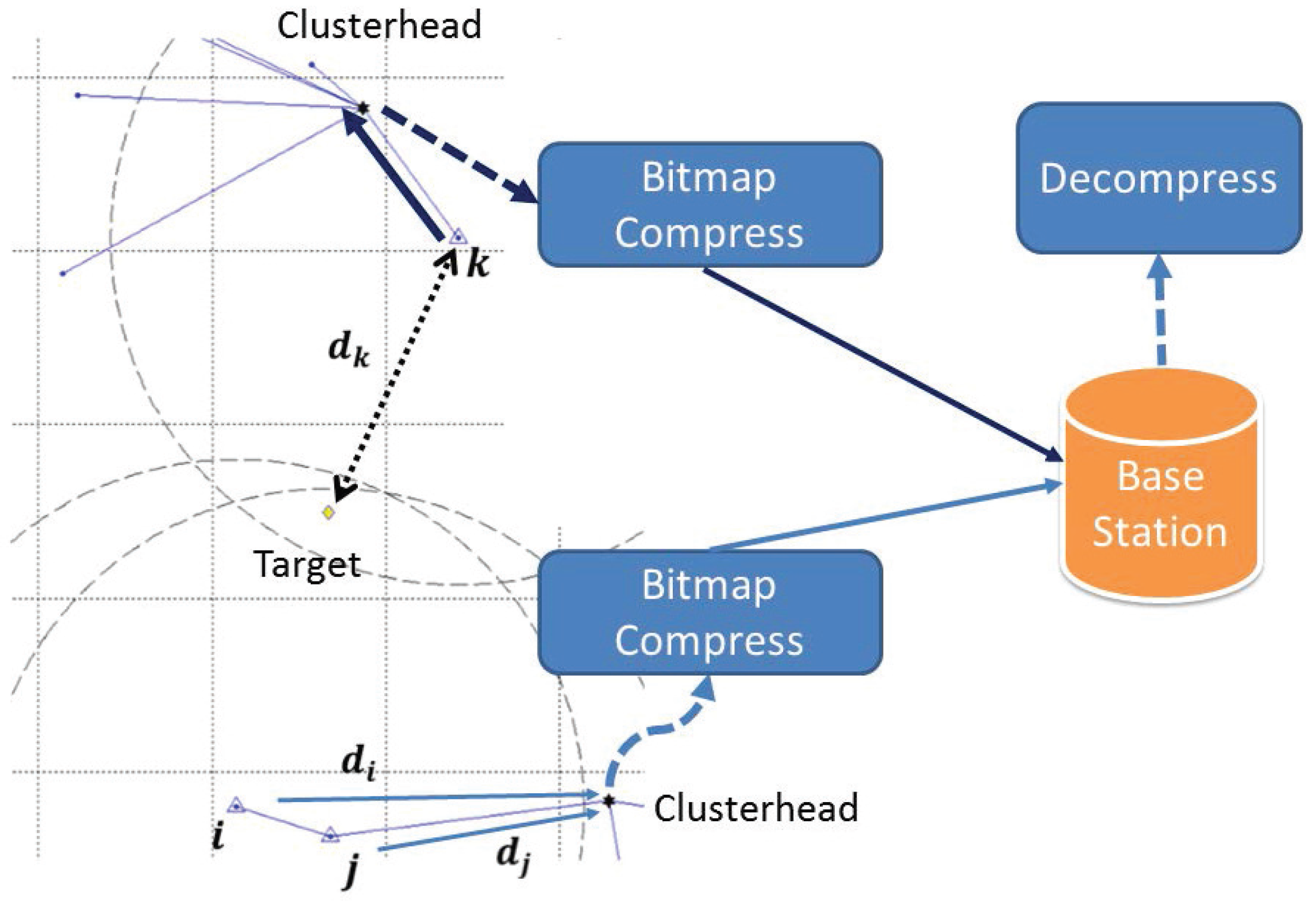
12] uses the distance measurements of sensor nodes to estimate the target location. The active sensors transmit their readings, including the estimated distances between them and the target and sensor ID to their clusterheads. The clusterheads gather the received data and then process the data in a centralized manner. The clusterhead processes the data by bitmap, which is a record indicating if the sensed data from a sensor can be approximated to the average value
μ of the data gathered by the clusterhead within a given compressing bound (e.g., using the standard deviation
σ to be the compressing bound). Therefore, if the value of a sensor reading is larger than the lower bound (
) and smaller than the upper bound (
), the data will be replaced by
μ, and the bit set to “0”, which means the data are compressed to
μ. If they are not, set the bit to “1”, and store the difference between the data and the average value for decompressing to the original data in the base station.
After scanning all of the data, there are a binary sequence (
i.e., data compression) and a decimal sequence (
i.e., the difference between the data and
μ) generated by the bitmap in the clusterhead. Then, the clusterhead transmits the sensor ID, average value and sequences of bitmaps to the base station. The base station decompresses the received data and uses them with the position of each active sensor to estimate the location of the target. The positions of active sensors and available information (e.g., distance measurements) form a possible area for the target (shown in
Figure 1), which means the target positioning will be influenced by the position of active sensors. The rationale is that if the active sensor is closer to the target, its weighting for estimation will be larger. Then, the result of position estimation will move toward the active sensor. Moreover, the number and the relative positions of the active sensors with respect to the target also influence the result of the position estimation. That is, if the active sensors are dense to a side, the position estimate will be much closer to the active sensors, and it may make the estimate far away from the target.
In this work, for the information processing approach, we apply the concept of bitmap in [
12] to compress the measurement information. The perspective of the binary sensor network inspires us to fully utilize the useful known information, which is not directly used by [
13]. Accordingly, the CTCI method aims to balance the tracking performance in terms of estimation accuracy and energy consumption. In this paper, our previous work, the Two-level Clustering Approach via Timer (TCAT) [
13] scheme, is used to build two-level clustering for the network architecture. Consequently, combining the Bayesian particle filter [
14] and local neighboring information, the proposed CTCI scheme is able to efficiently complete the tracking task.
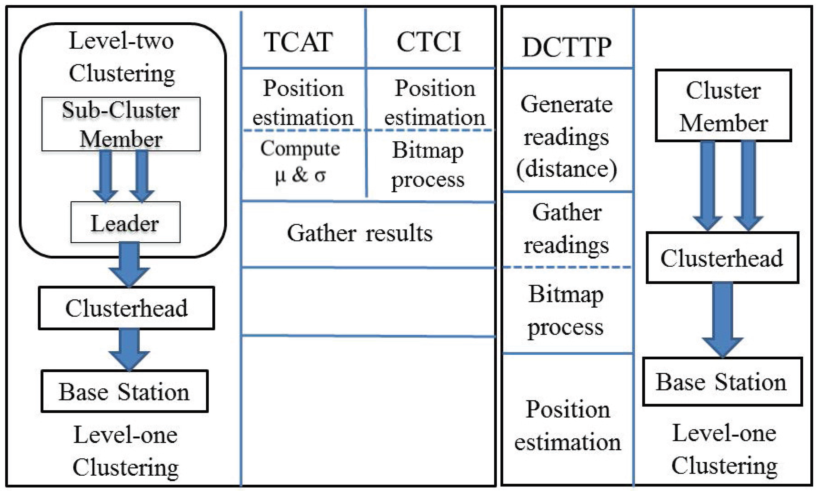
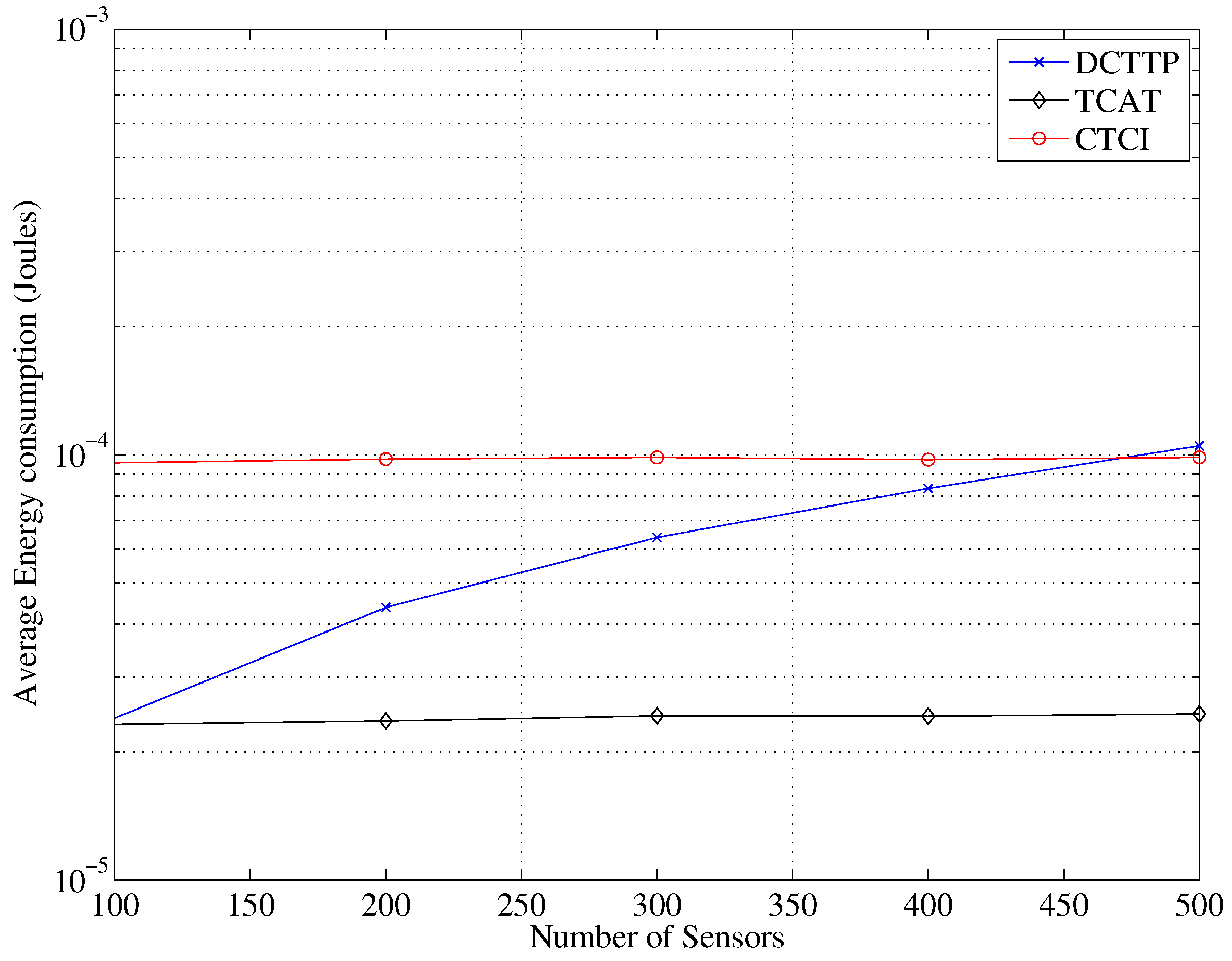
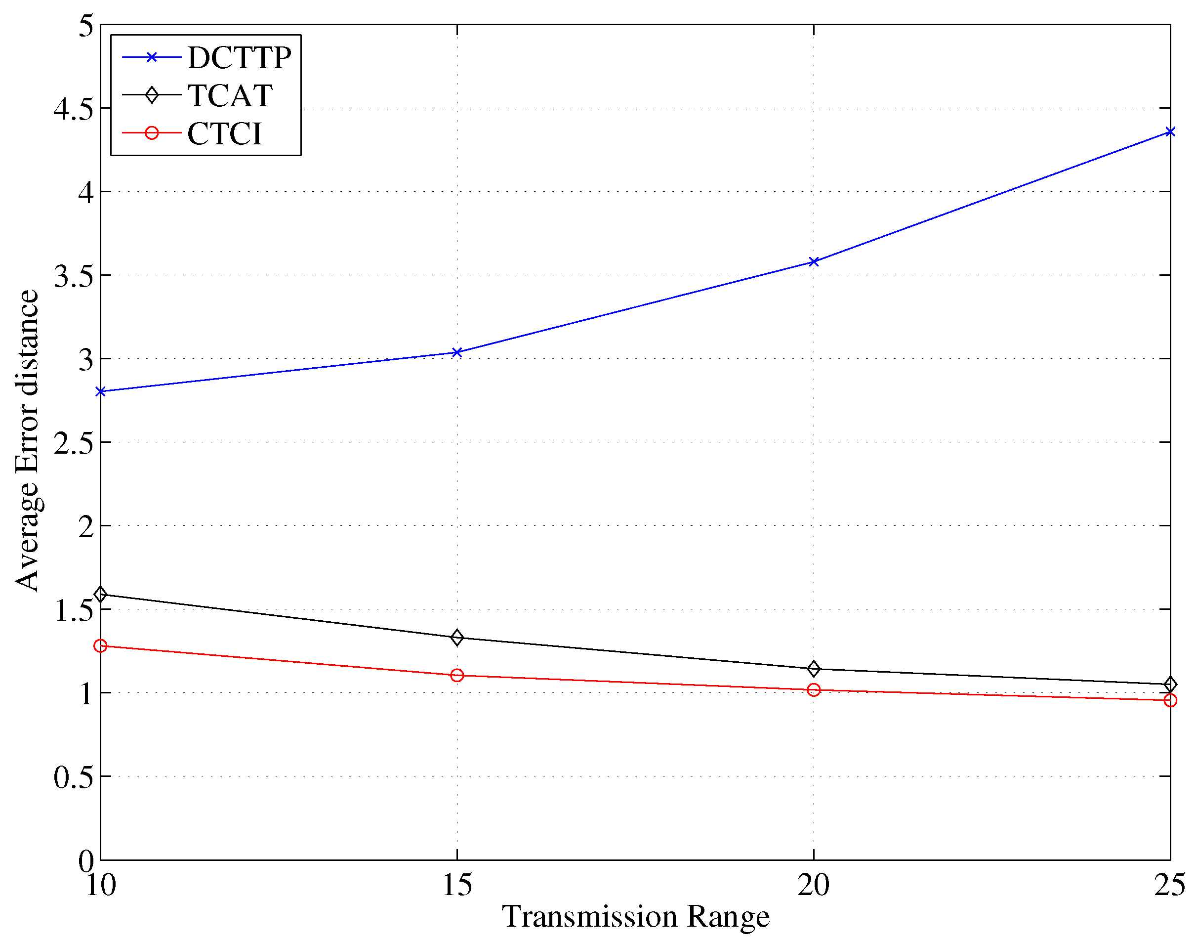
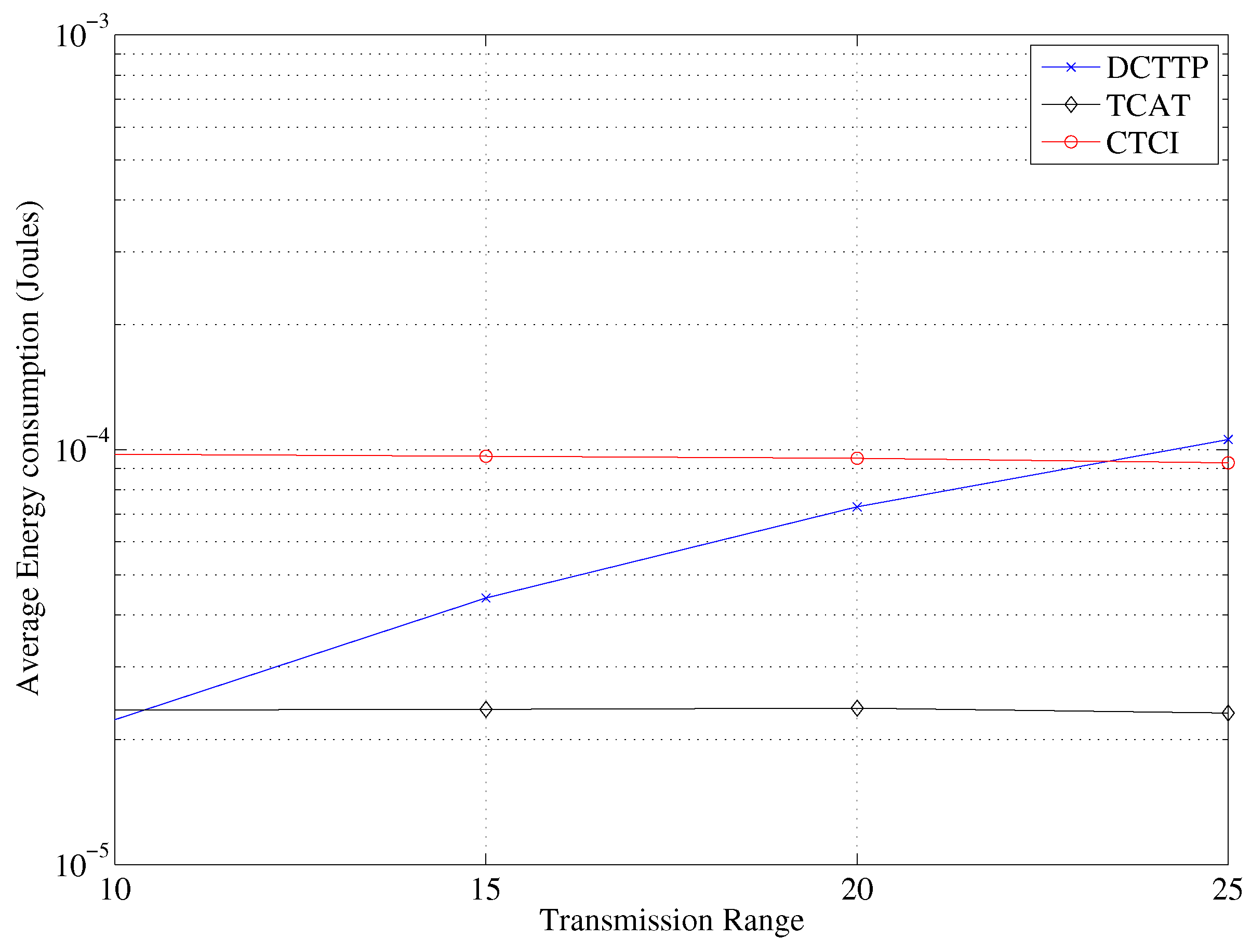
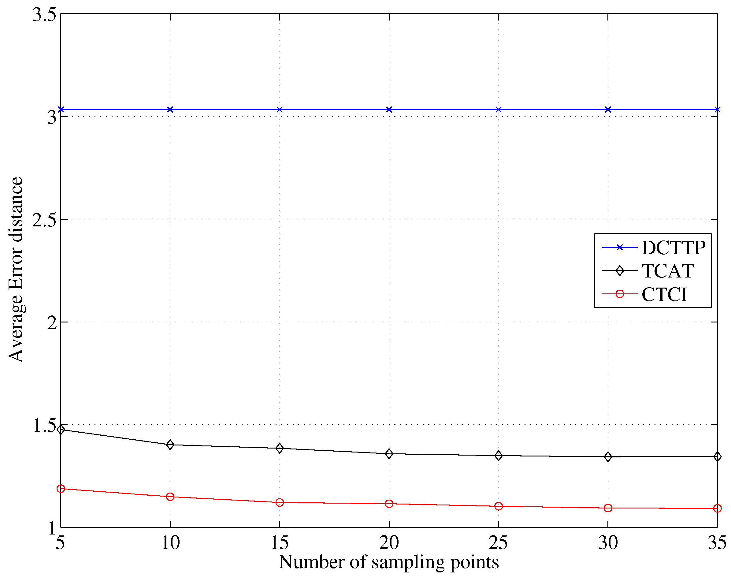
Here, we compare the information processing model of TCAT, CTCI and DCTTP for target tracking (shown in
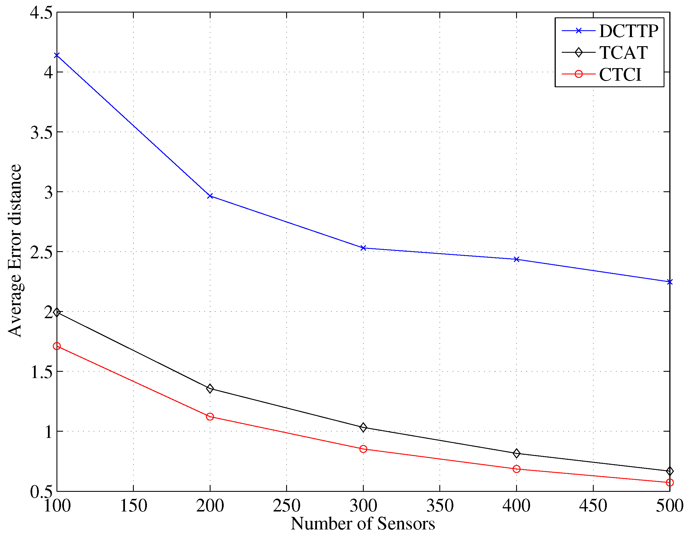
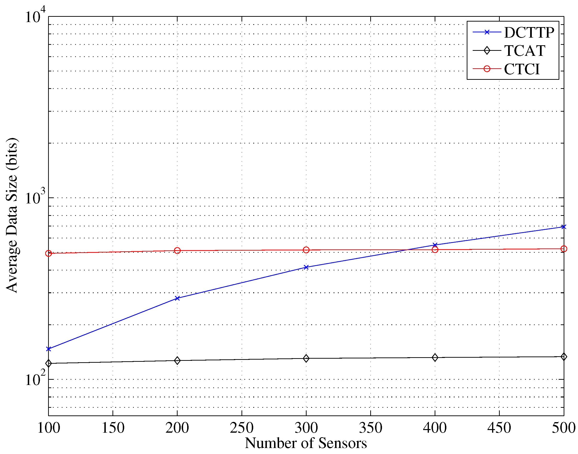
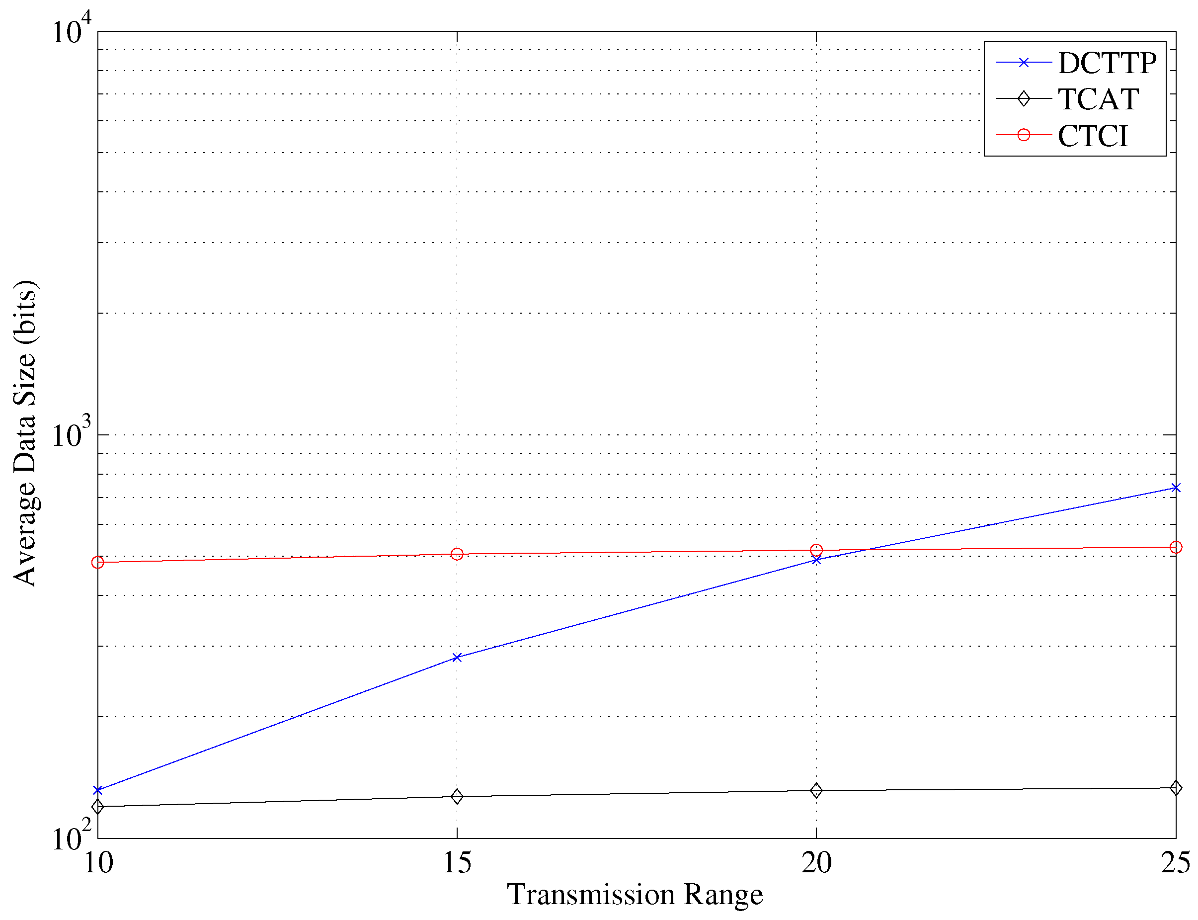
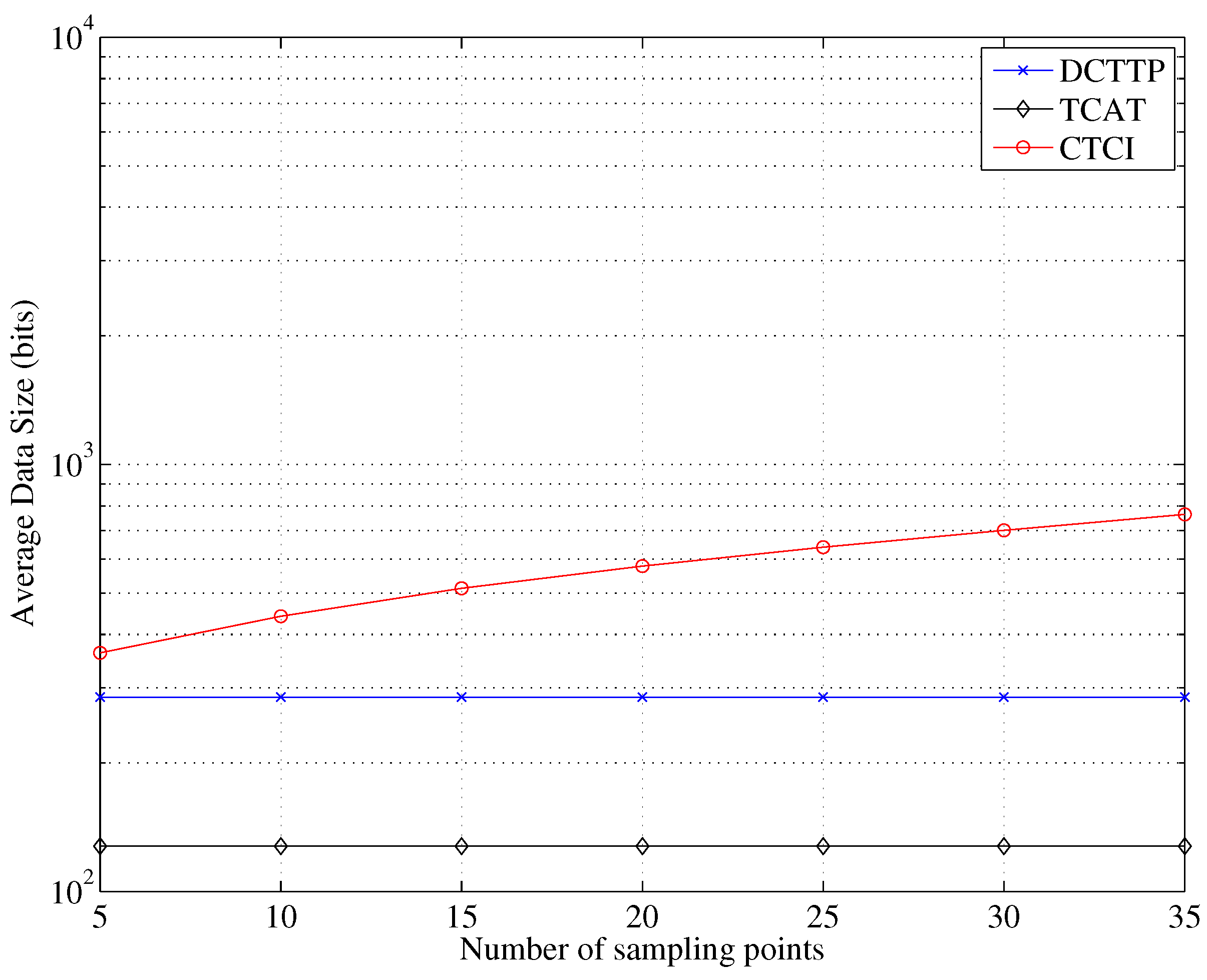
Figure 2). Observe that there is only a single hierarchy in DCTTP, but two hierarchies in TCAT. Thus, TCAT focuses on organizing the active sensors triggered by the target. Consequently, the system of TCAT is more stable and efficient than that of DCTTP, and TCAT can instantly acquire the result of target tracking at Level 2 clustering. Although there are many protocols proposed for target tracking, the network architecture and information processing problems are not considered simultaneously [
7,
8,
9,
10,
11,
15,
16,
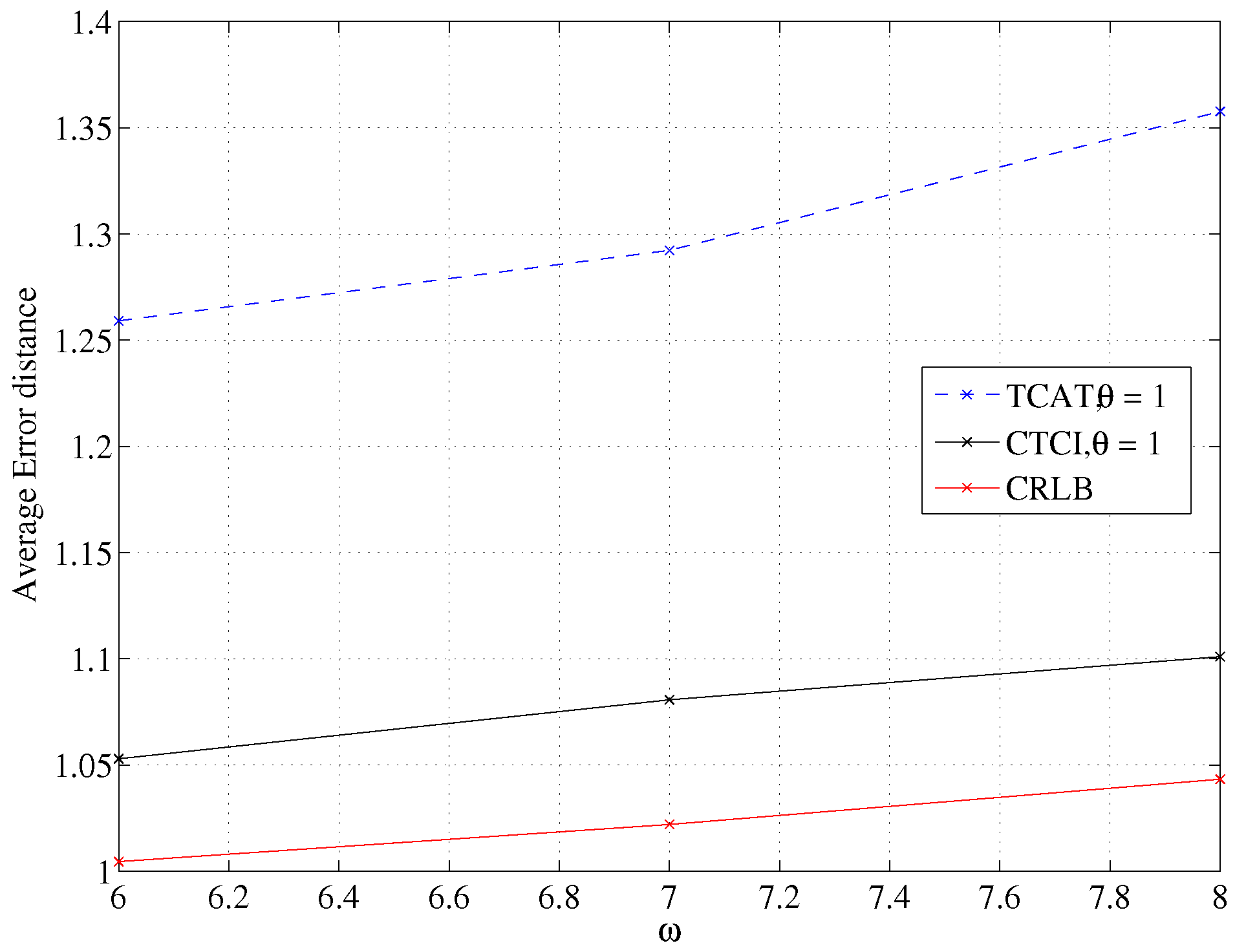
17]. Hence, we tackle the tracking task and the data processing problem based on the network architecture in TCAT. Even though the energy consumption and the data size of CTCI are slightly higher than that of TCAT and DCTTP in some cases, the system of CTCI is able to adaptively provide the measurement distribution via information compression, not just describing the target position with a single estimate. Notice that the TCAT scheme can be considered as a special case of CTCI with a large compression bound, which compresses the samples to the mean. Moreover, the estimation accuracy and the integrality of the tracking result of CTCI are better than that of TCAT (improved by
) and are much better than that of DCTTP (improved by
). We investigate the trade-off between the tracking quality and the energy consumption in
Section 5.
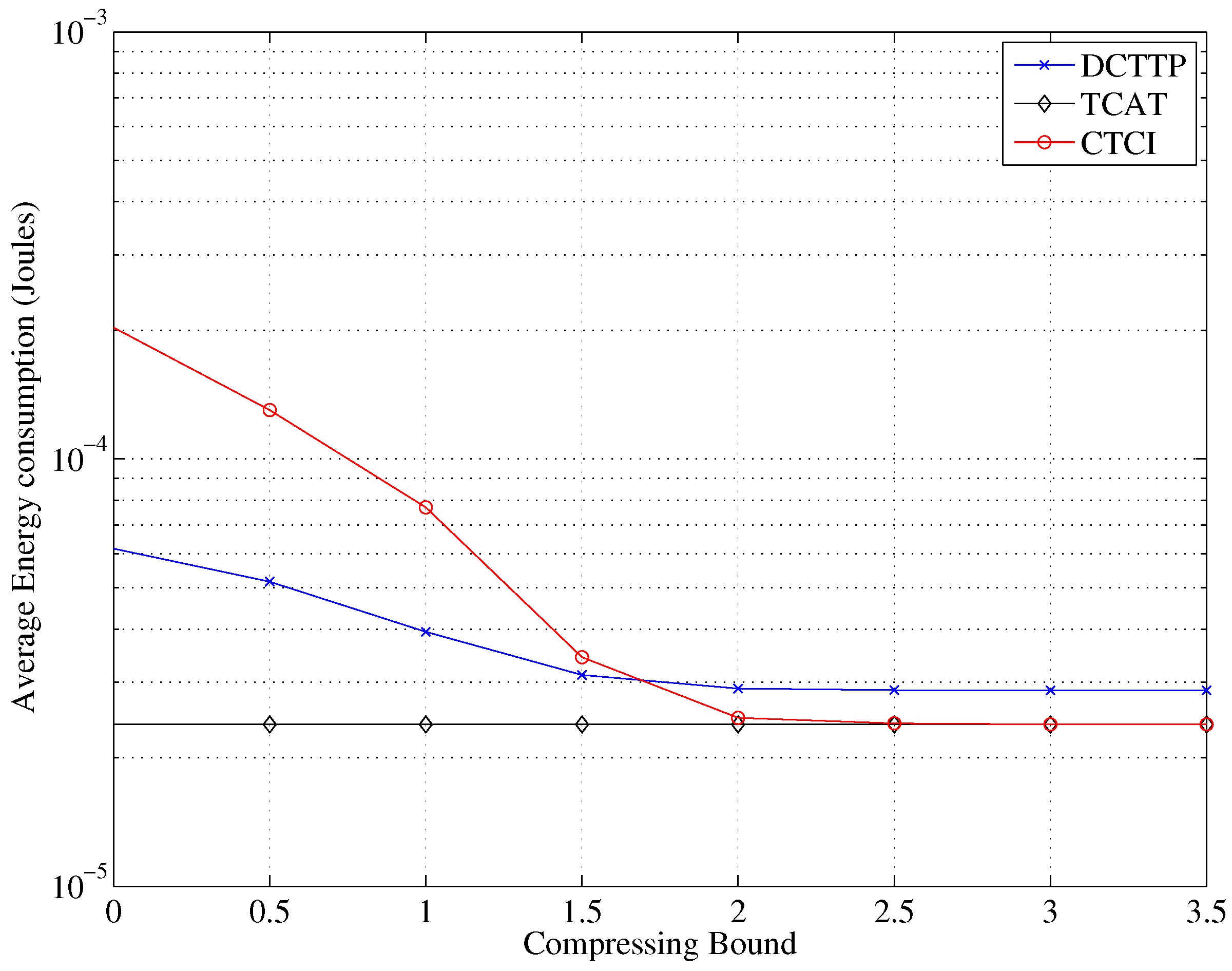
3. Data Processing Schemes
This section discusses the proposed data processing scheme, Cooperative Tracking via Compressing Information (CTCI), including the tracking method, information processing model, information flow and the meaning of the location estimation. First, we introduce the network architecture and TCAT, which is the basic model of the proposed CTCI data processing scheme. Secondly, we compare and contrast the DCTTP and TCAT schemes. Finally, a new data processing scheme, CTCI, is proposed to balance the distortion of the processed data and the energy consumption.
3.1. Problem Statement
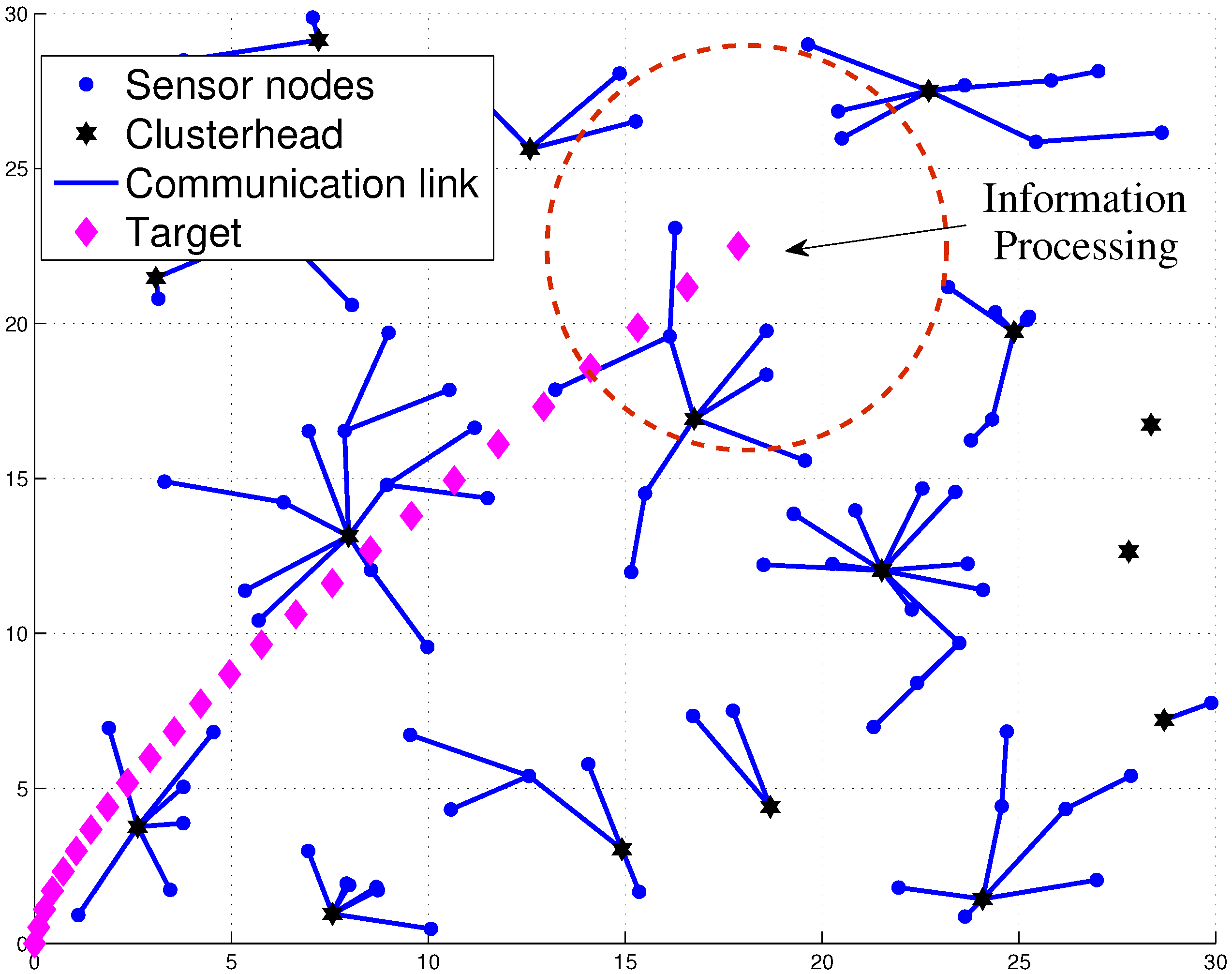
Figure 3 shows an example of target movement with 25 time steps. In the presence of the target, to achieve load-balancing tracking, an important issue of target tracking is how to collect the desired data and to perform efficient information processing. Denote a sensor with tracking responsibility as an active sensor. Otherwise, a sensor is marked as an inactive sensor. Thus, referring to the Level 1 clustering in
Figure 3, the Level 2 clustering utilizes a dynamic clustering scheme to adaptively form a local sub-cluster with active sensors for the tracking task in a distributed manner (
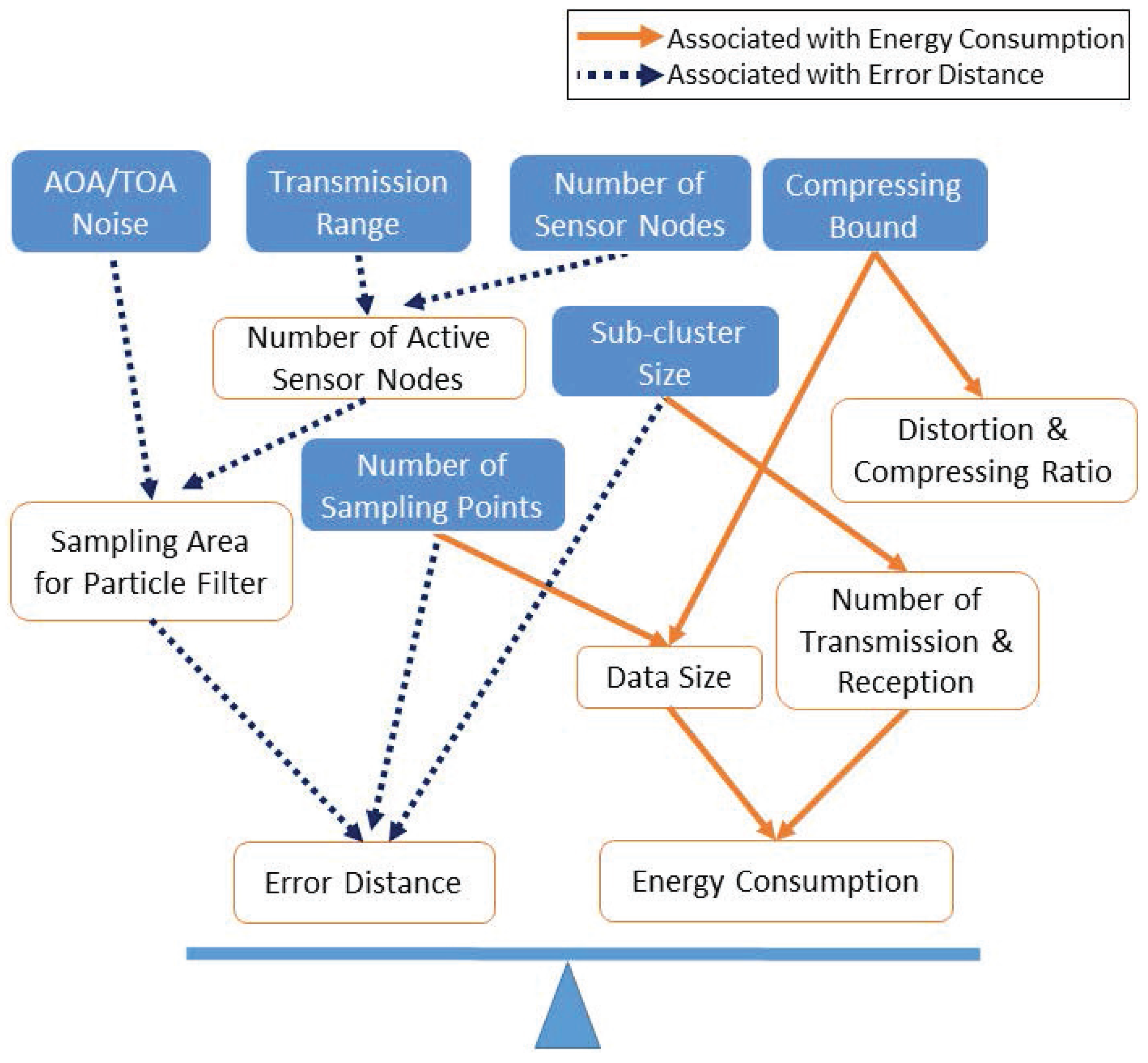
Figure 4). Since there is a trade-off between estimation accuracy and energy consumption, this work aims to investigate the network performance on data size and energy conservation for target tracking from an information processing perspective. The main assumptions are: (1) all sensor nodes are assumed to be homogeneous with their fixed position information in a strongly-connected network; (2) the noise model is the zero-mean Gaussian noise measurement model; (3) Angle-of-Arrival (AOA) information or hybrid Time-of-Arrival (TOA)/AOA information is applied to perform target tracking; and (4) the target broadcasts a message for measurement purposes periodically. Note that these assumptions may be applied to locate objects (e.g., patients or animals) in healthcare or habitat monitoring scenarios.
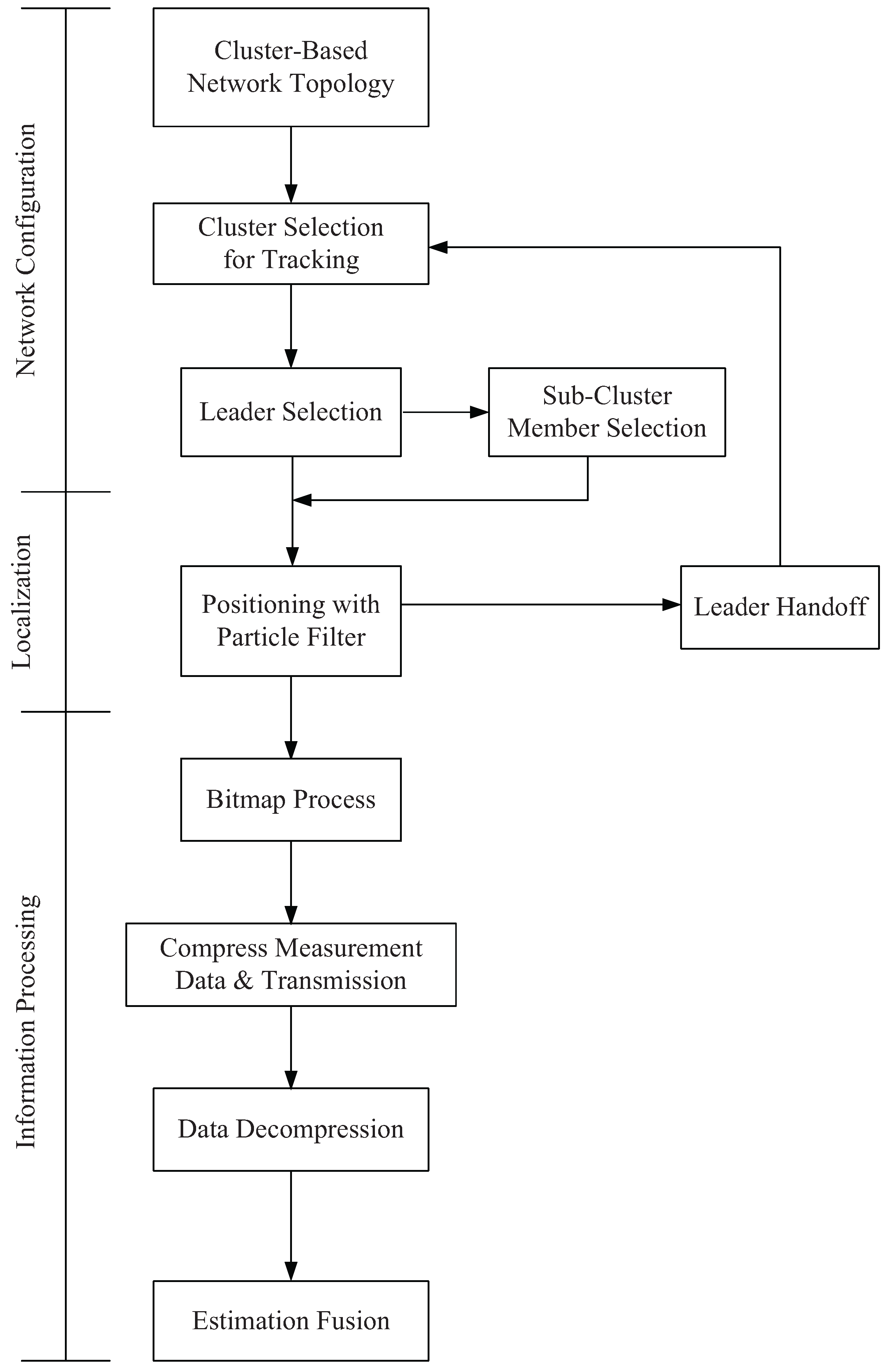
Accordingly, as depicted in
Figure 5, the CTCI scheme performs target tracking in three major phases: (1) network configuration; (2) target positioning; and (3) information processing. The following subsections describe each phase, respectively.
3.2. Network Configuration and TCAT
This section describes the fundamental system configuration of CTCI. To achieve distributed scheduling target detection and tracking, a two-level clustering (
i.e., a hybrid static/dynamic clustering scheme) is applied to deal with the control of network operations and to handle the tracking task, which is based on our previous works, the Clustering Algorithm via Waiting Timer (CAWT) scheme [
18] and the TCAT scheme [
13]. During the network initialization phase, sensors may apply the CAWT to establish a Level 1 network architecture (
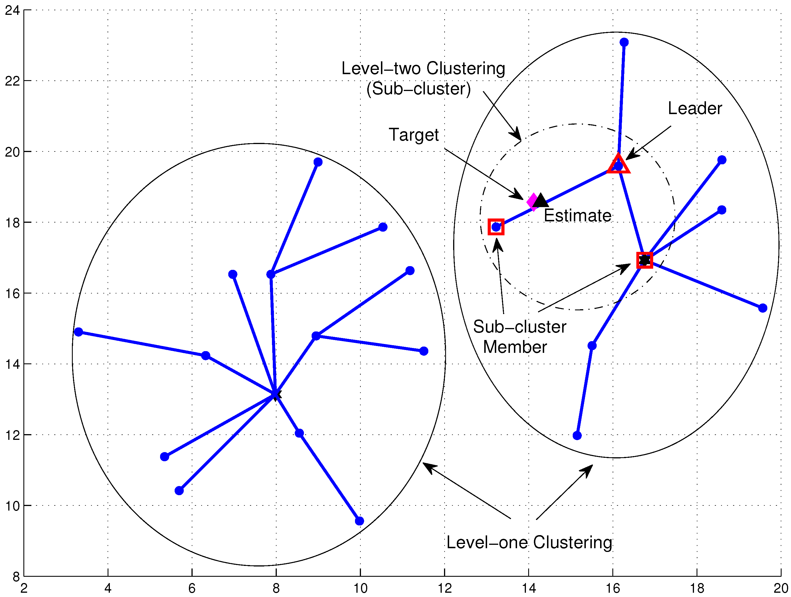
Figure 3). In order to handle the impact of the target movement, the TCAT scheme may be applied to form a sub-cluster with tracking responsibility and allow each sub-cluster member to locally locate the target in a distributed manner.
Figure 4 shows an example of leader and sub-cluster member selection. Therefore, the TCAT scheme may be applied to select the sensors with tracking responsibility and build a Level 2 network architecture. Notice that the information flow is bi-directional (
i.e., it goes through the sub-cluster members to the leader and then to the clusterhead, and vice versa).
3.3. Target Positioning
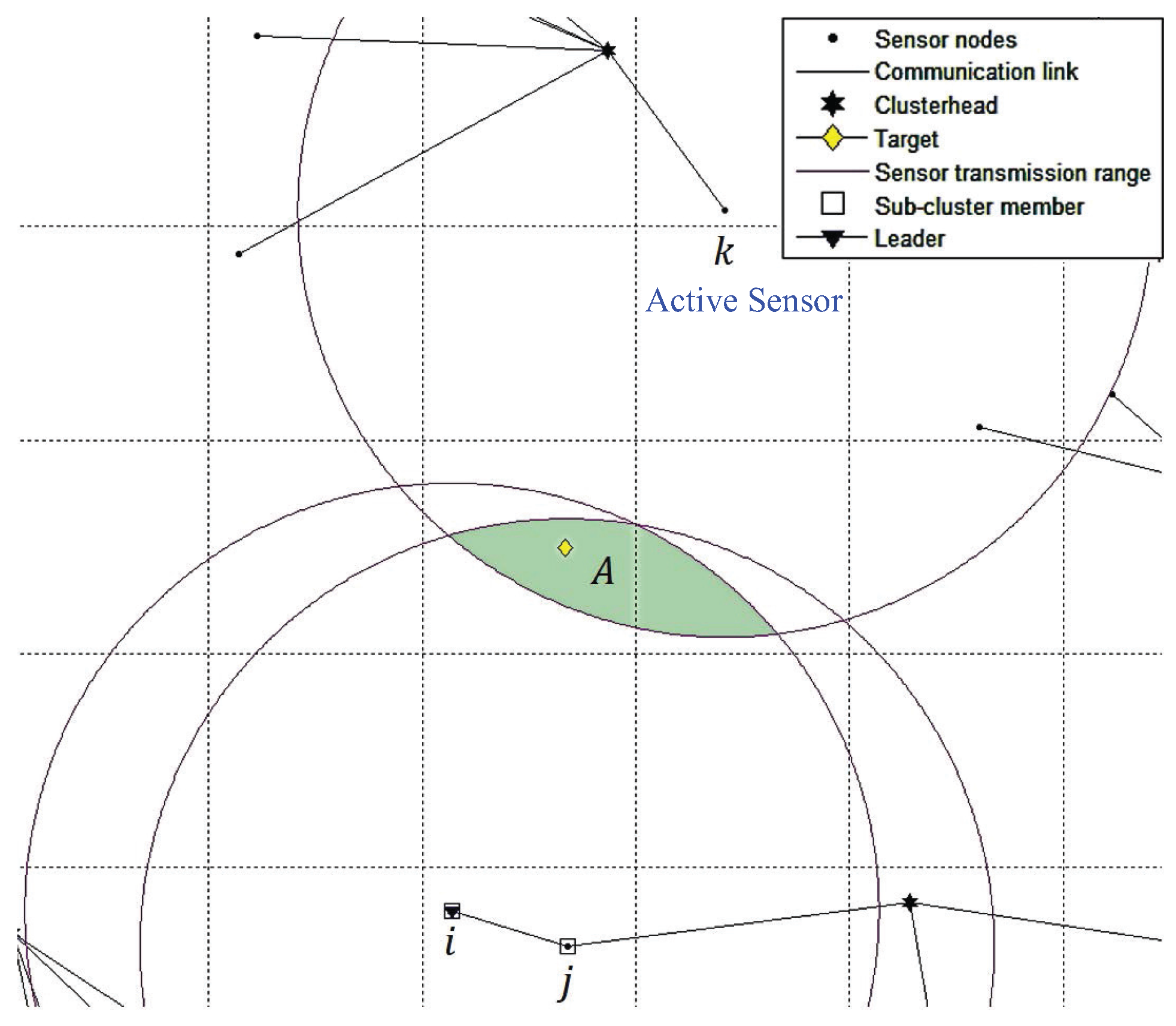
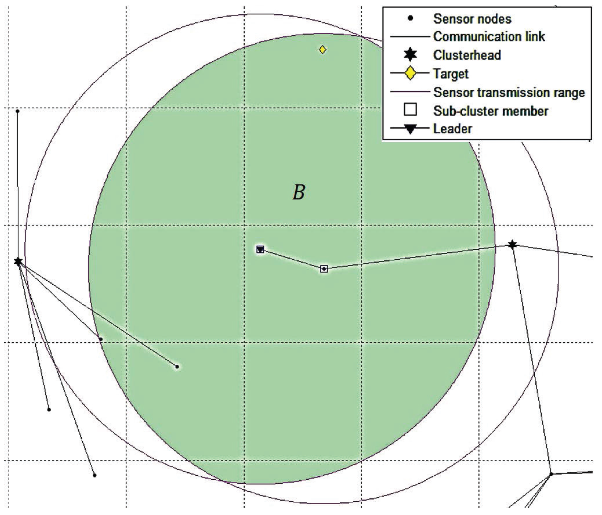
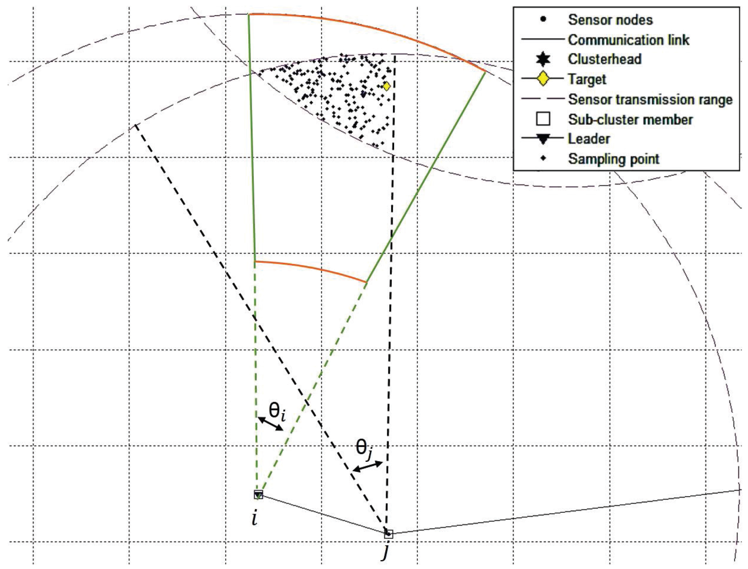
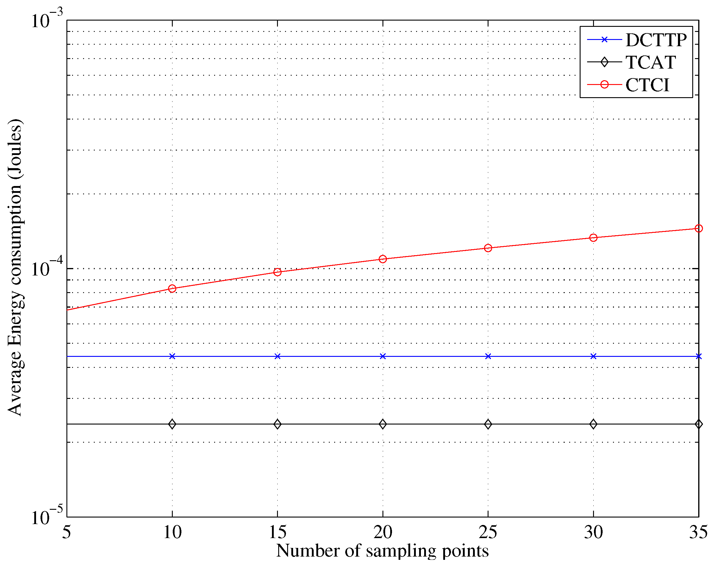
The major difference between TCAT and CTCI is the bounding area formed by the different numbers of active sensors. In TCAT, the bounding area is determined by the active sensors in the same cluster. In CTCI, the bounding area is determined by not only the active sensors in a single cluster, but also the active sensors in other clusters. It is worth mentioning that including the active sensors in different clusters can effectively decrease the scope of the bounding area for sampling. The bigger the distance between the active sensor and the others, the smaller the intersection area of the transmission range of the active sensor will be, which suggests that we can provide a better sample area for particle filtering and even use fewer sampling points for the tracking task as the sample area decreases. Observe that in
Figure 6, we can see that an active sensor node is added to form the bounding area A in CTCI, which is smaller than the bounding area B in TCAT (as shown in
Figure 7). Accordingly, we may use a smaller number of samples (
Figure 8) to achieve a comparable estimation accuracy with particle filtering.
On the basis of the refined sample area, the position estimation method is as follows:
Create a random sample , from the refined sample area at time step .
Each random sample is passed through the state Equation (1) to obtain samples at time step
.
where the system noise
is a sample drawn from the Gaussian noise, Φ is characterized by the mobility model and Γ is assumed to be an identity matrix.
Upon receipt of the noisy measurement
, evaluate the likelihood of each prior sample and obtain the normalized weight of each sample. Therefore, after updating the weights of the likelihood function
for each sample, the normalized weights yield:
Based on the normalized weights, it generates a new sample set by performing sampling with replacement from the set (), which describes the distribution of the position estimate.
Note that the noise model is the zero-mean Gaussian noise measurement model. A typical setting of the prior parameter values is described in
Section 5.1.1. For obtaining the distribution of position estimate, each tasking sensor sends the mean and variance of the distribution to the tasking leader.
3.4. Information Processing and Data Management
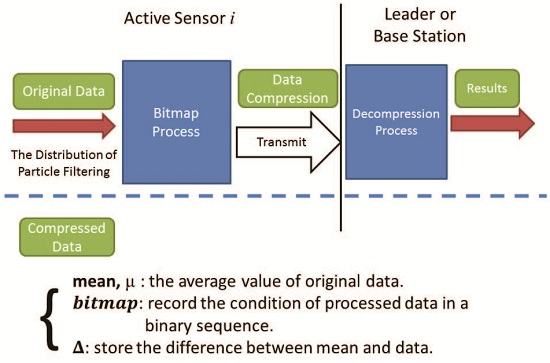
Figure 9 depicts the conceptual procedures of information processing. The concepts and techniques (in the upper row) represent the processing mechanisms of active sensors and the leader, respectively. Upon obtaining the distribution of the target position by using a particle filter in an active sensor, data analysis is performed to explore the distribution properties, execute information compression and then transmit the processed data to a leader (or a base station). Afterwards, a leader (or a base station) may apply the received processed data (in the lower row) to generate a distribution, which roughly corresponds to the estimation distribution. The proposed algorithm uses the bitmap process and statistical properties to execute data processing, which consists of the following five steps:
Preliminary settings∼ Each tasking sensor performs target positioning with Bayesian filtering of N samples, which leads to a target position estimate at time step k, , where , .
Configuring the bitmap of ∼ Each tasking sensor computes the average , , , and generates the value of compressing bound, and , where η is an adjustable factor to trade off the compression ratio and positioning accuracy.
Compression of ∼ As shown in
Figure 10b,c, scan and compress
and
(using
and
as examples). Hence, if (
), then bit(
) = 1 and
. Similarly, if (
), then bit(
) = 1 and
. Afterwards, the tasking sensor (
i.e., a sub-cluster member) transmits the compressed data (
, △(
), △(
),
,
).
Data decompression∼ As shown in
Figure 10a, decompress the received data by scanning
, △(
) and △(
). If bit(
) = 1, then
; otherwise,
.
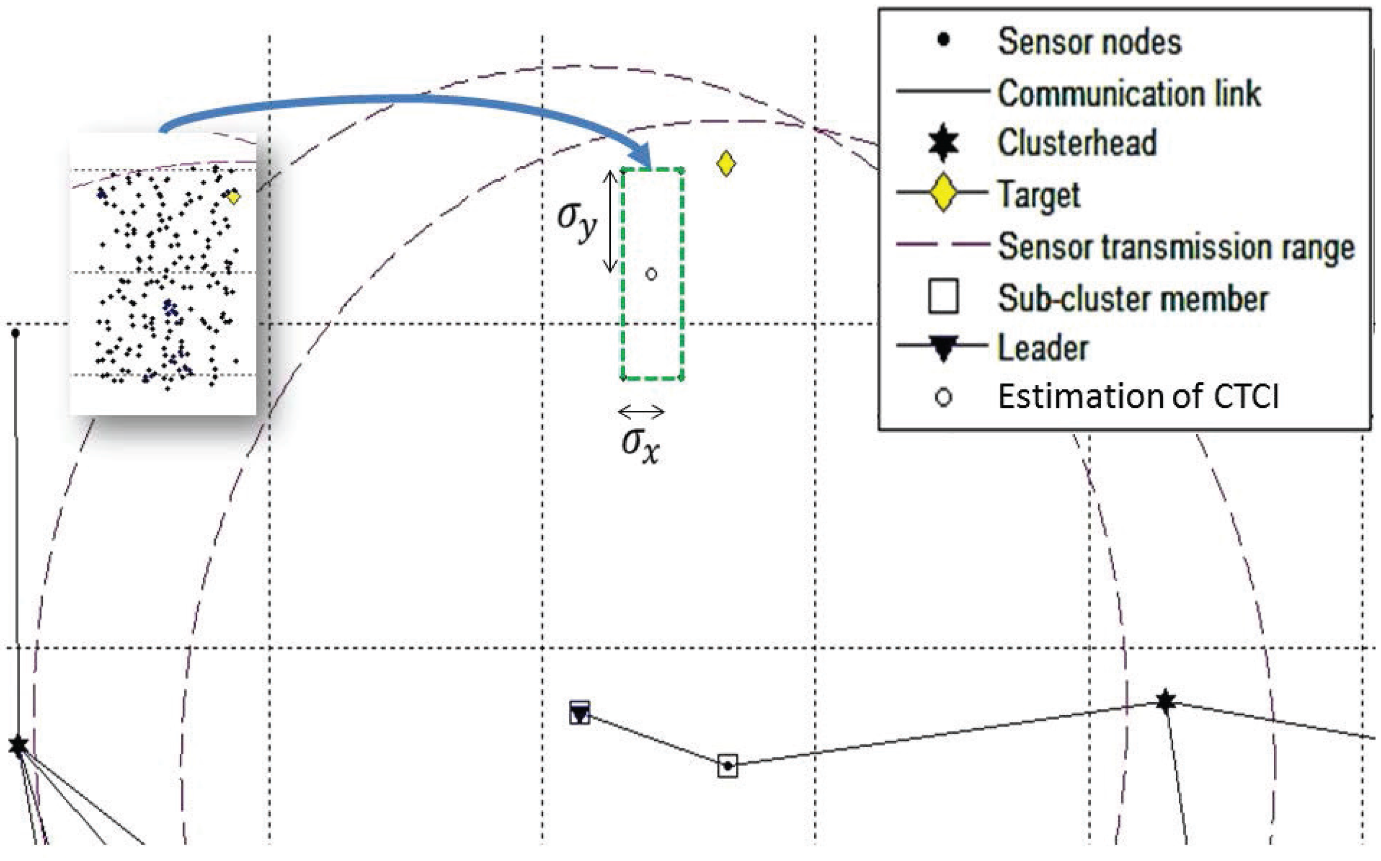
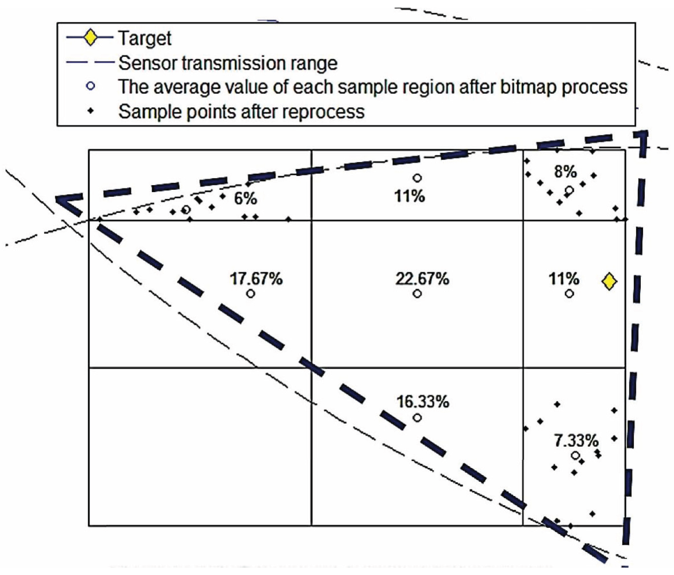
Estimation fusion∼
Figure 11 shows the external contour of the sample region and the distribution of the decompressed data. The leader node scans the information of each sample sub-region. Let
be the target appearance probability of sample region
m, which yields
(
), where
is the number of sample points in region
m and
is the total number of sample points. Let
be the average estimate of sample region
m. Accordingly, we obtain the location estimate
.
Therefore, the information processing of the CTCI scheme is completed.
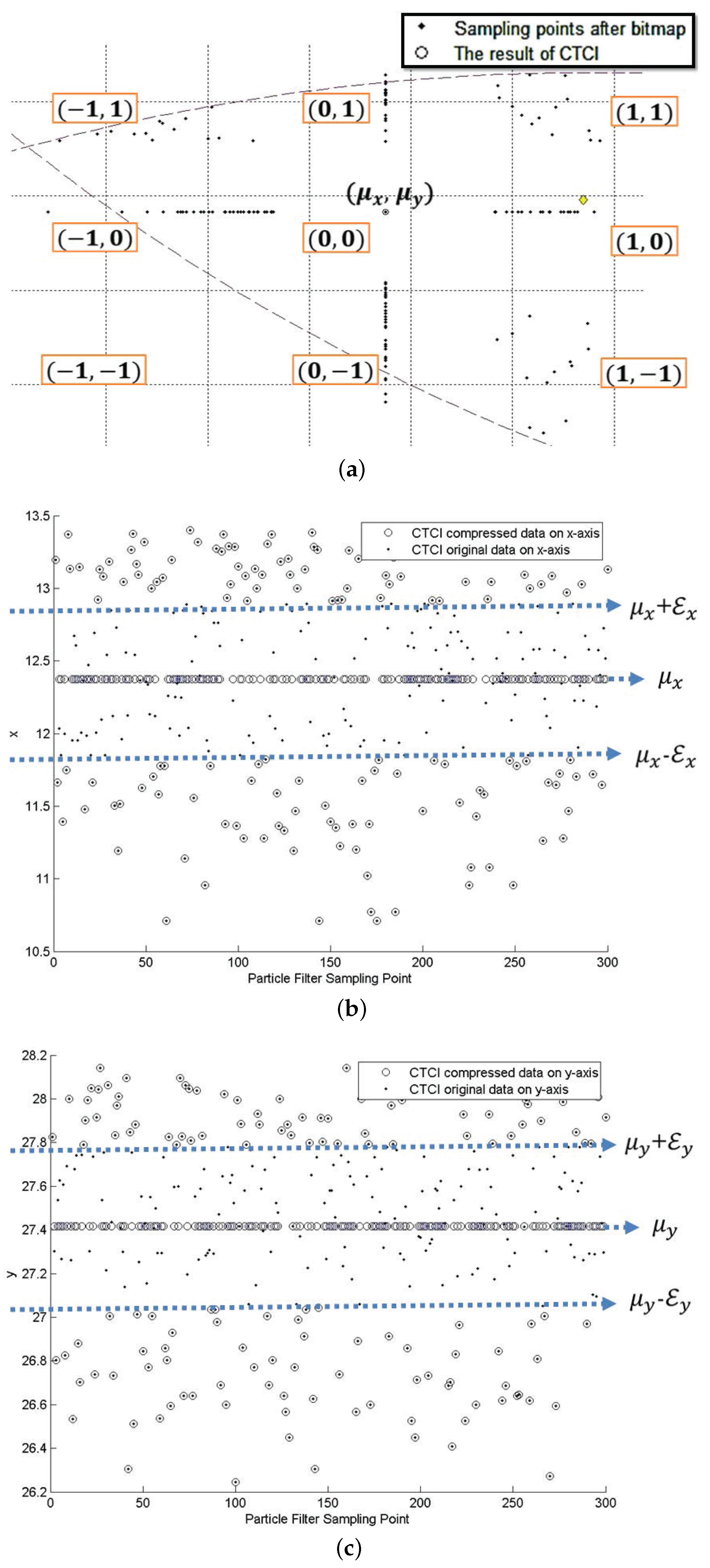
Compared to DCTTP (a one-dimensional data processing method), the bitmap process in CTCI is a two-dimensional data processing method. Thus, the sampling points after the bitmap process will have several combinations the for
x and
y coordinates. From
Figure 10a, we observe three basic combinations of the sampling points: (1) (0,0) means both the values of the
x and
y coordinates are approximated to the average value at the same time; (2) (1,0) or (0,1) means a value of the
x or
y coordinate is approximated to the average value, but the other one is not; (3) (1,1) means both values are not represented by the average value. The minus “−” means that the value of the
x or
y coordinate is smaller than the average value. Thus, the sample region is divided into nine parts by the bitmap process. In
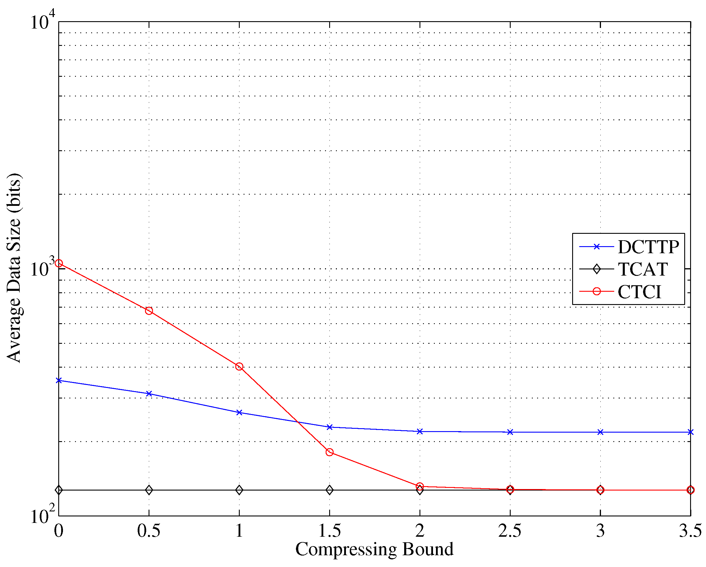
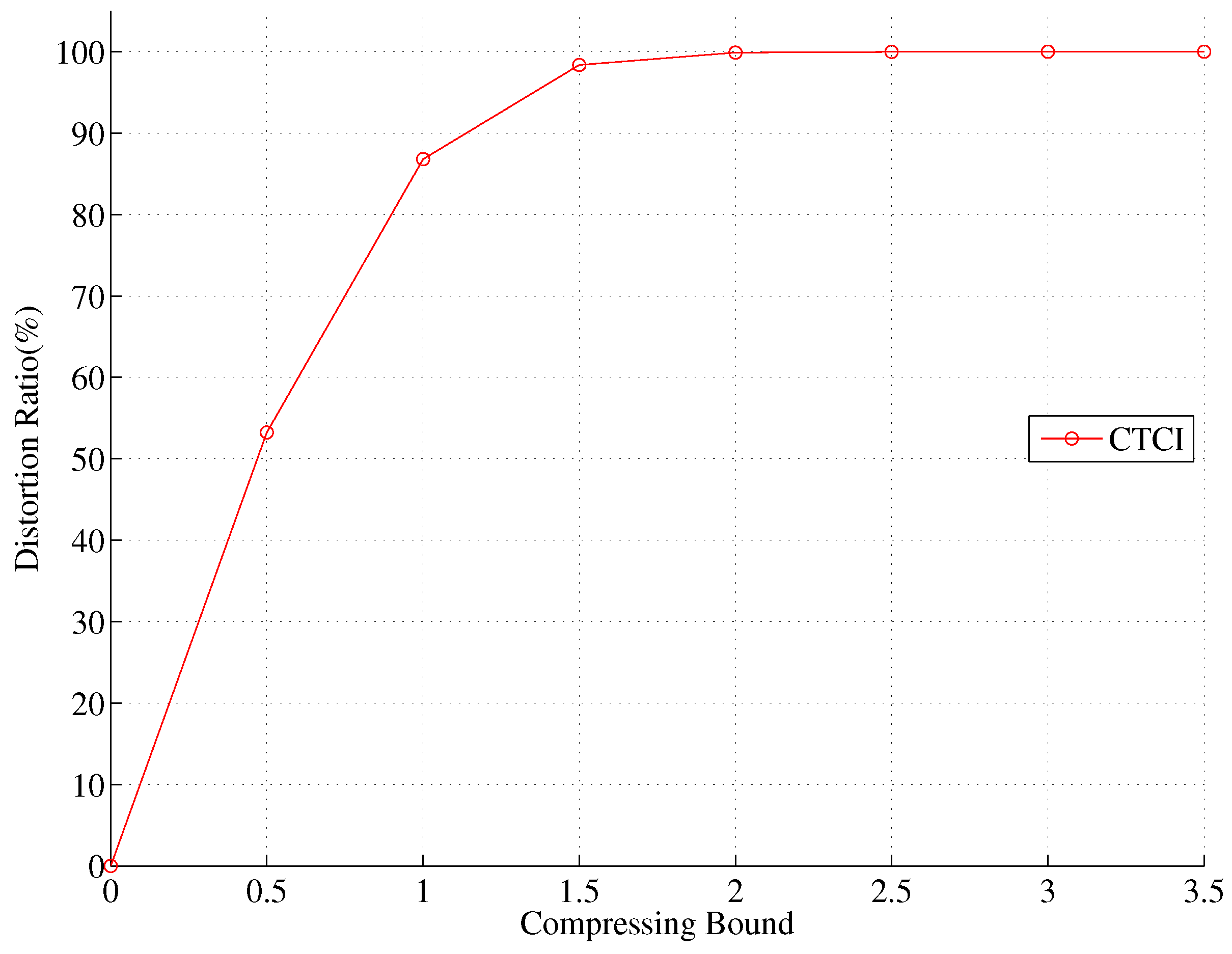
Figure 10b,c, the distributions of the original and compressed sampling points show the distortion of the
x and
y coordinates, respectively. The data within the compressing bound are represented to the average value, which causes the distortion. Thus, there is a trade-off between the energy consumption and the extent of distortion.
Therefore, each sub-cluster member transmits the compressed data, including (1) the average value and the standard deviation of the original sample points and (2) the differences between the sample points and the average value, to the leader node. Afterwards, the leader may transmit the position estimate to the base station through clusterheads and gateways in a multi-hop manner or directly disseminate the data from the clusterhead to the base station. In the leader node, the processed data are decompressed, and the external contour of the sample region is depicted by recovering the original sample points associated with (1,1), (−1,1), (1,−1), (−1,−1) representations as the results for data processing. The meaning of the result is shown in
Figure 11, which means that the result of the target positioning is not only just a position estimation, but also a similar area of the original region for sampling. After obtaining the distribution of the position estimate, each tasking sensor sends the mean and variance of the distribution to the tasking leader.
6. Conclusions
This paper presents an information compression scheme for target tracking. Comparing the proposed CTCI method to the TCAT and DCTTP methods, the simulation results show that the proposed CTCI scheme can adaptively control the estimation performance and closely reflect the relationship between the distortion of tracking results and energy consumption. Considering the system parameters (e.g., transmission range, the number of sensor nodes, compressing bound, the number of sub-cluster size and the number of sampling points), at the slight cost in data size and energy consumption, the tracking accuracy of CTCI is superior to those of TCAT (improved by ) and DCTTP (improved by ). Therefore, many trade-offs between the system parameters need to be considered in each scheme. In future work, we will explore a more effective and robust compression scheme, evaluate the compression complexity and quality and adjust the tactics of the two-level clustering to further reduce the data size, maintain the desired estimation quality and achieve energy conservation.


