
Atmospheric Correction of Satellite GF-1/WFV Imagery and Quantitative Estimation of Suspended Particulate Matter in the Yangtze Estuary

Abstract
:1. Introduction
2. Materials
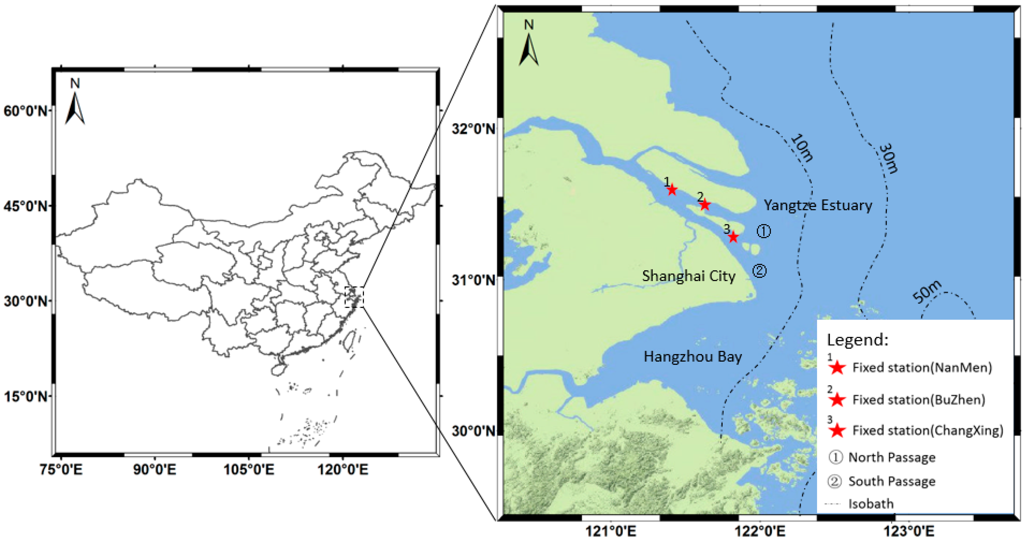
2.1. Study Area
2.2. Satllite Data
2.3. In Situ Data
3. Methods
3.1. GF-1/WFV Imagery Processing
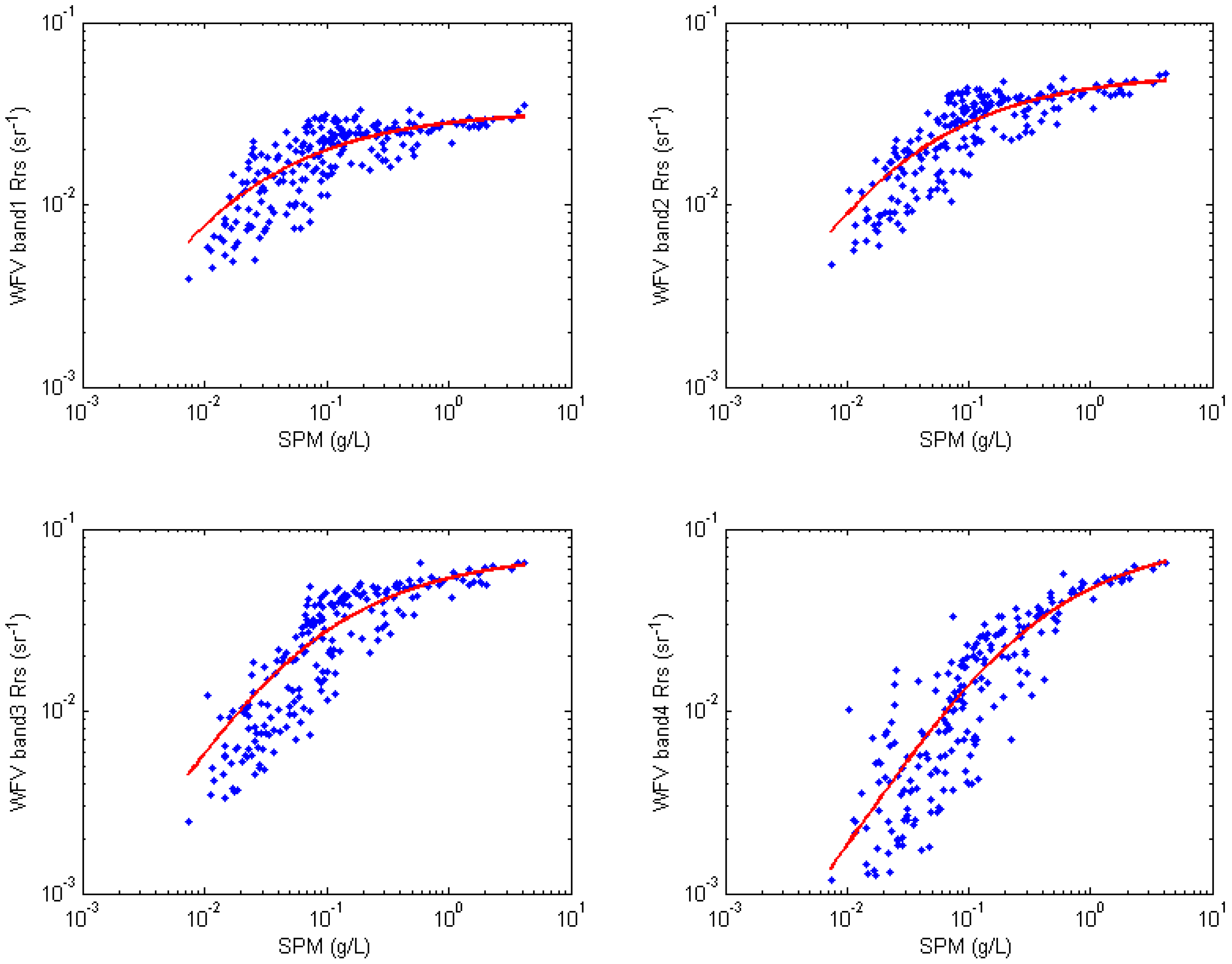
3.2. Recalibration of SERT Model
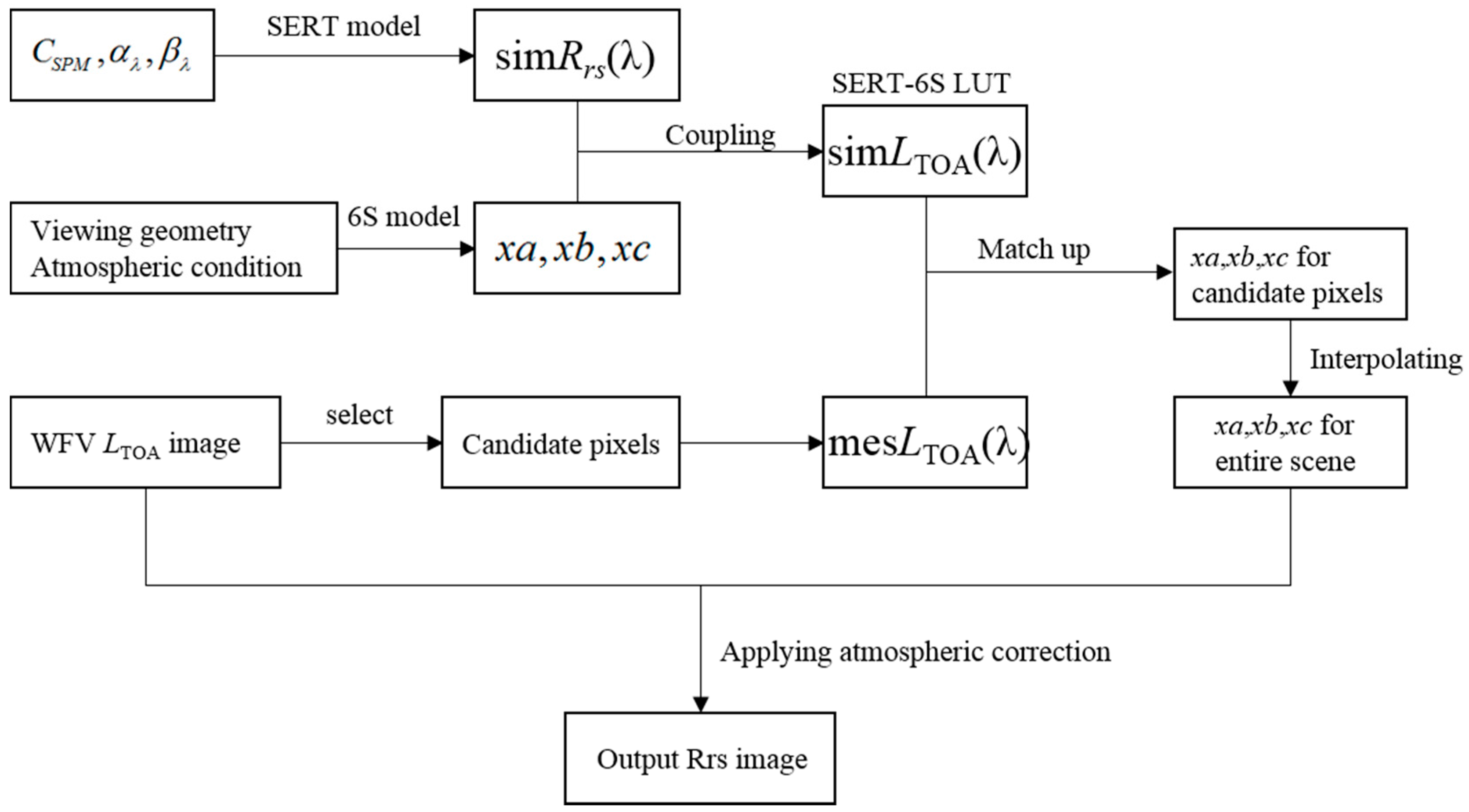
3.3. Atmospheric Correction Scheme
4. Results and Discussion
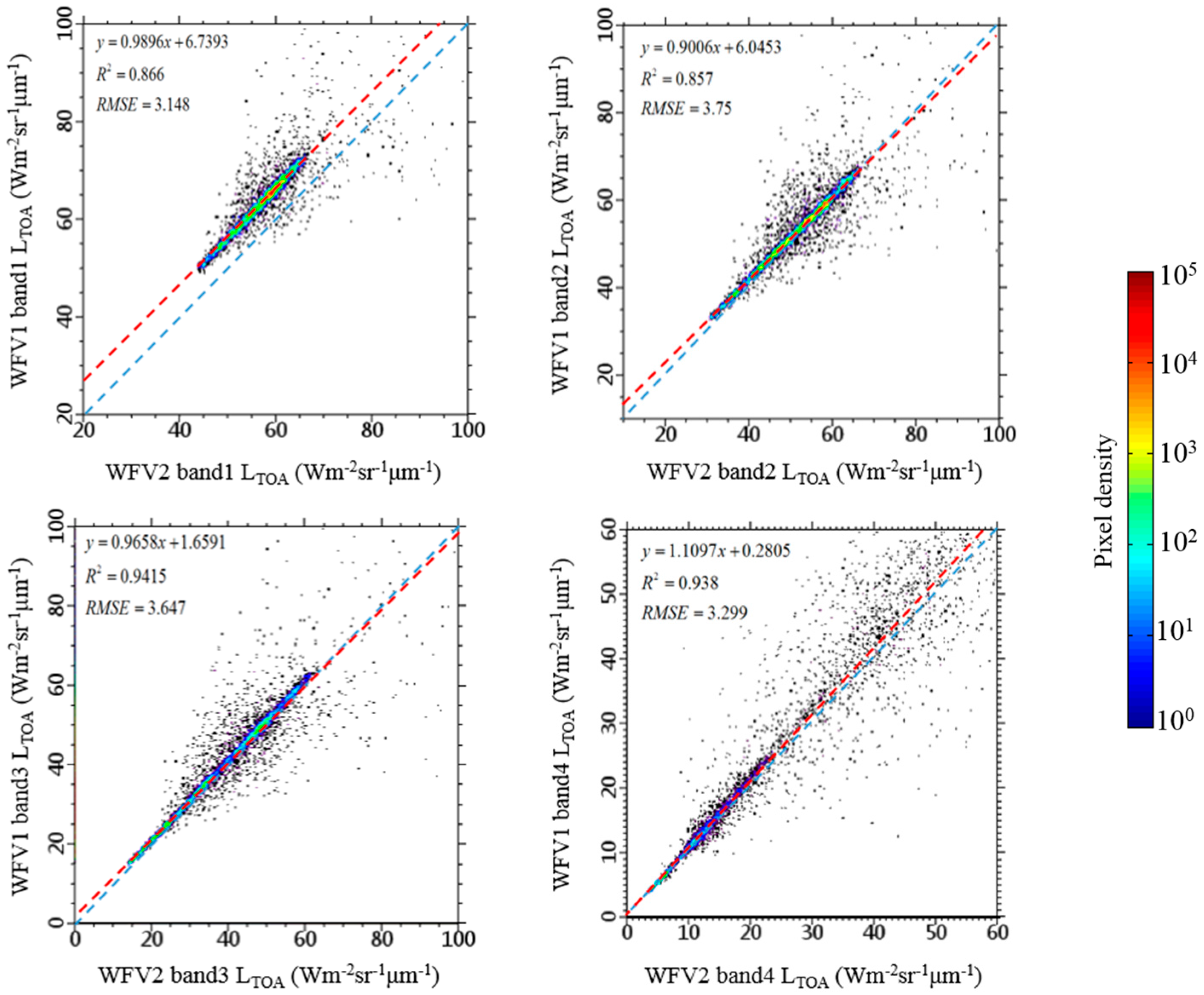
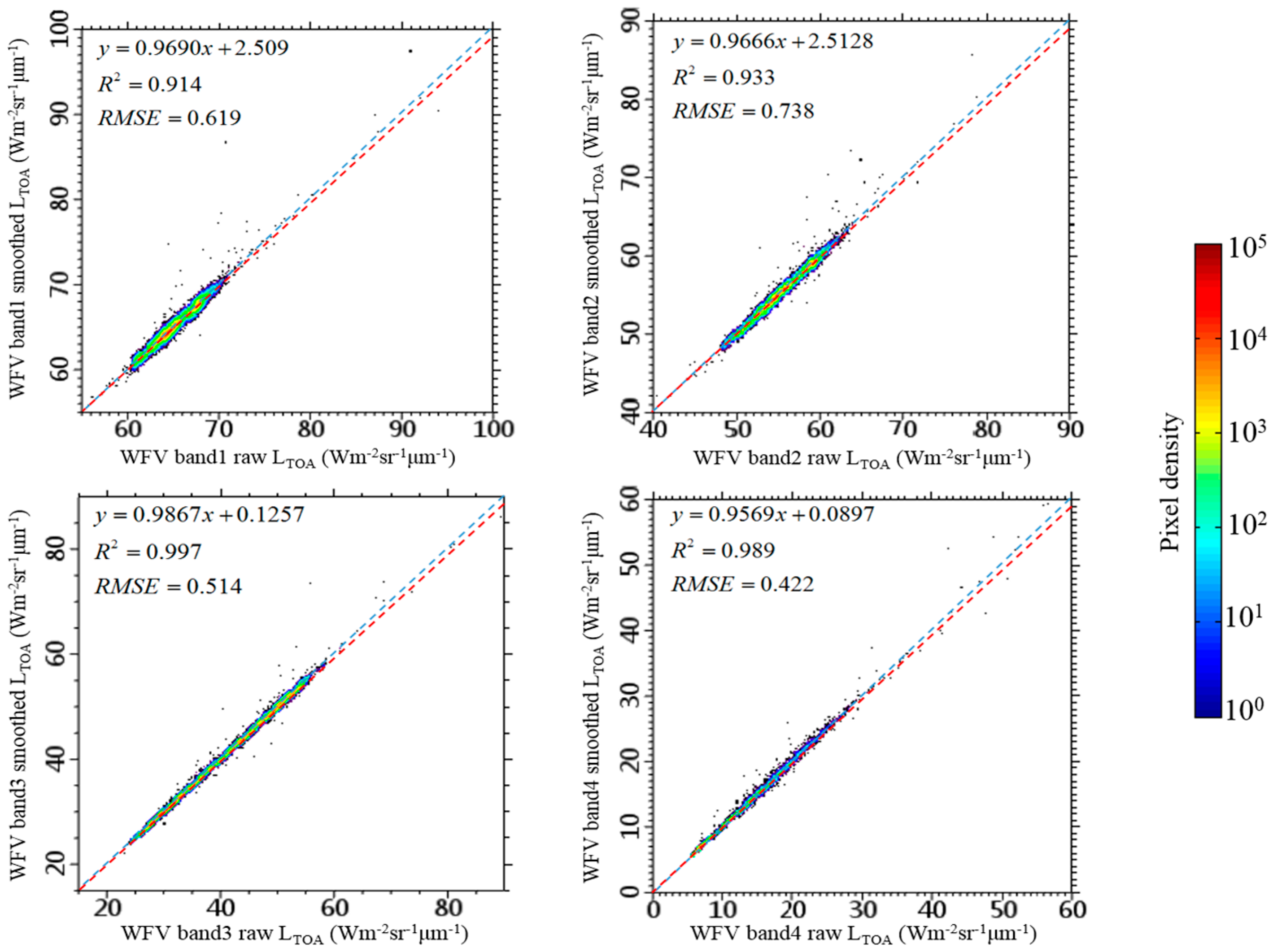
4.1. GF-1/WFV Imagery Processing
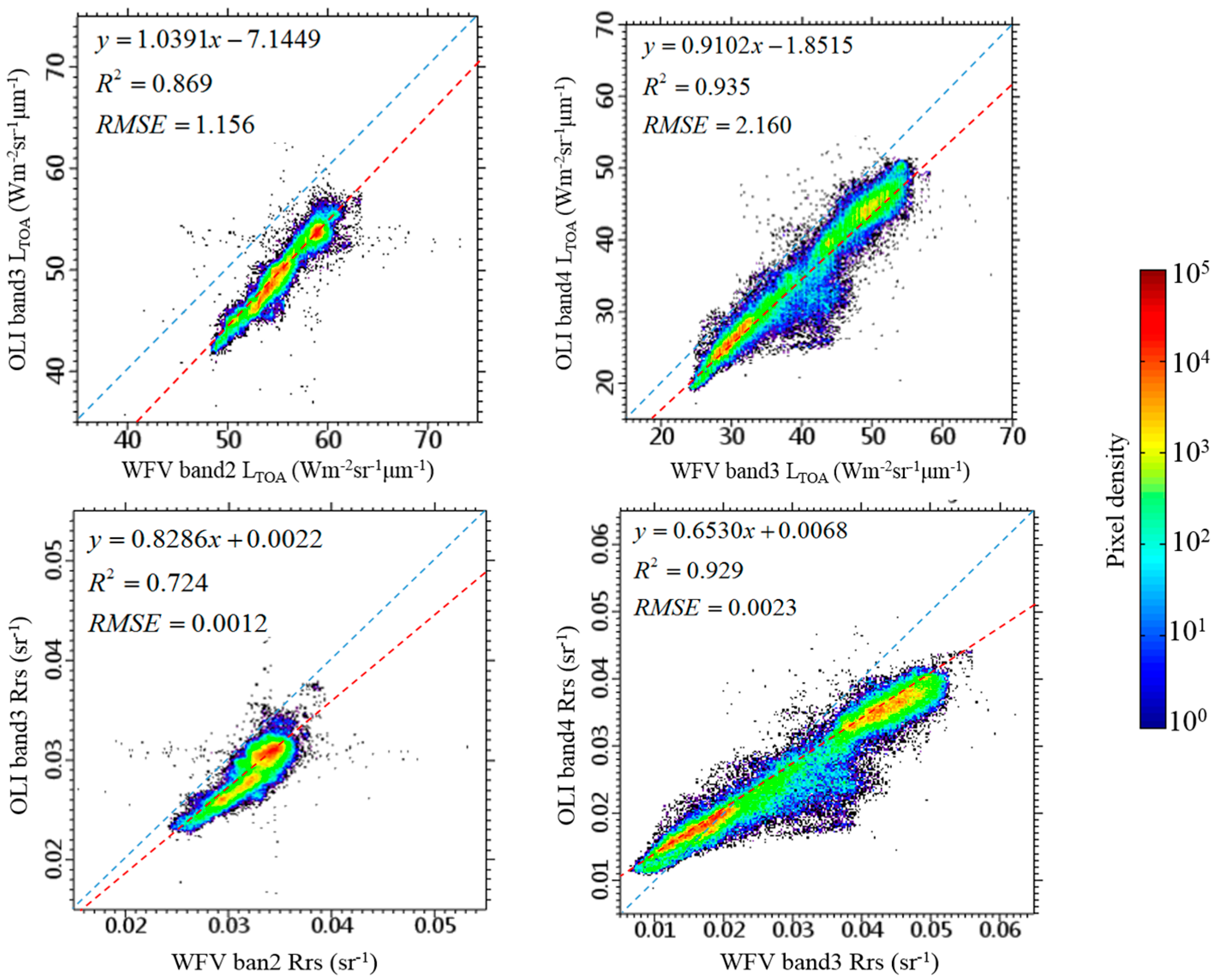
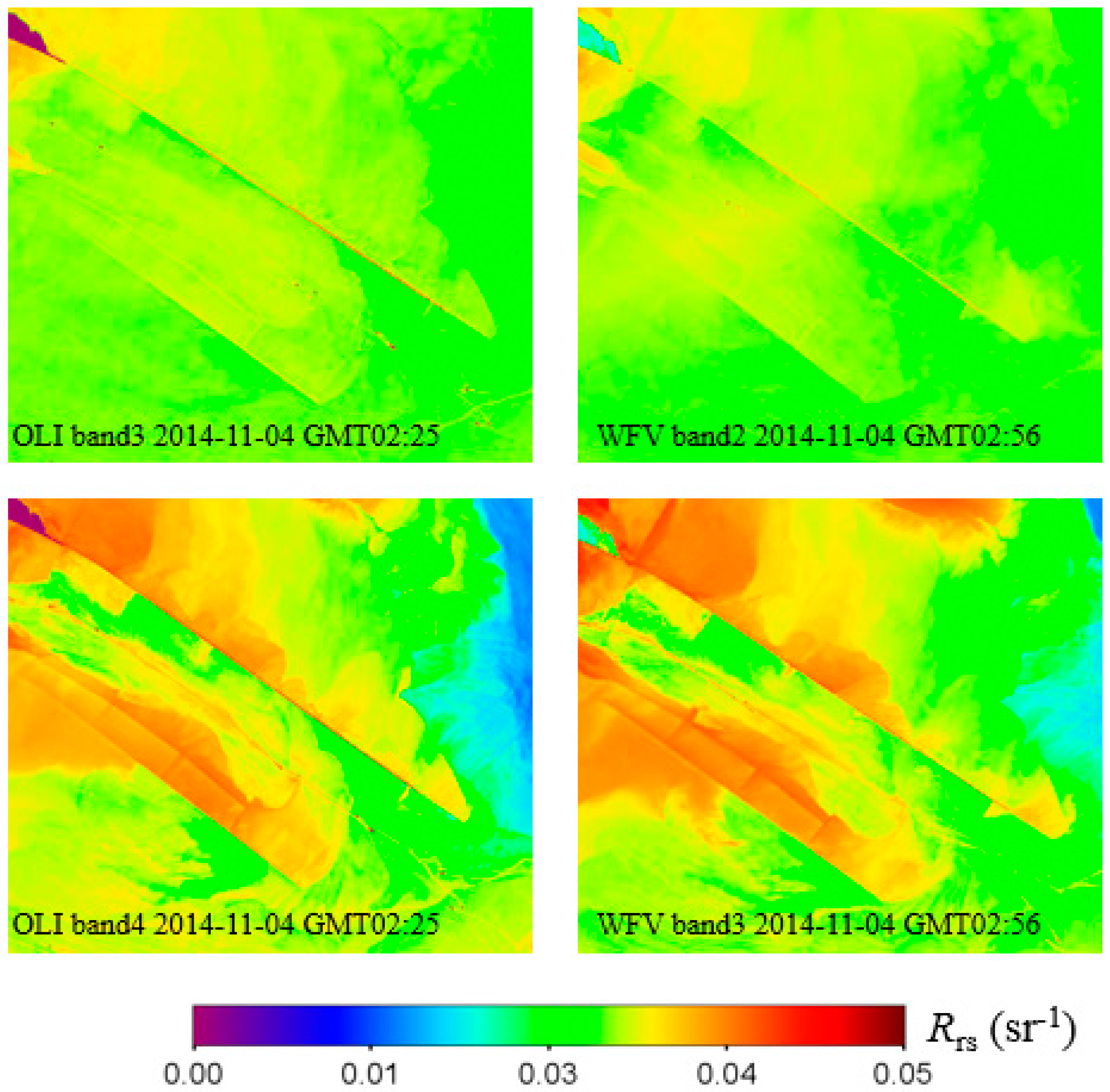
4.2. Atmospheric Correction and Intercomparison
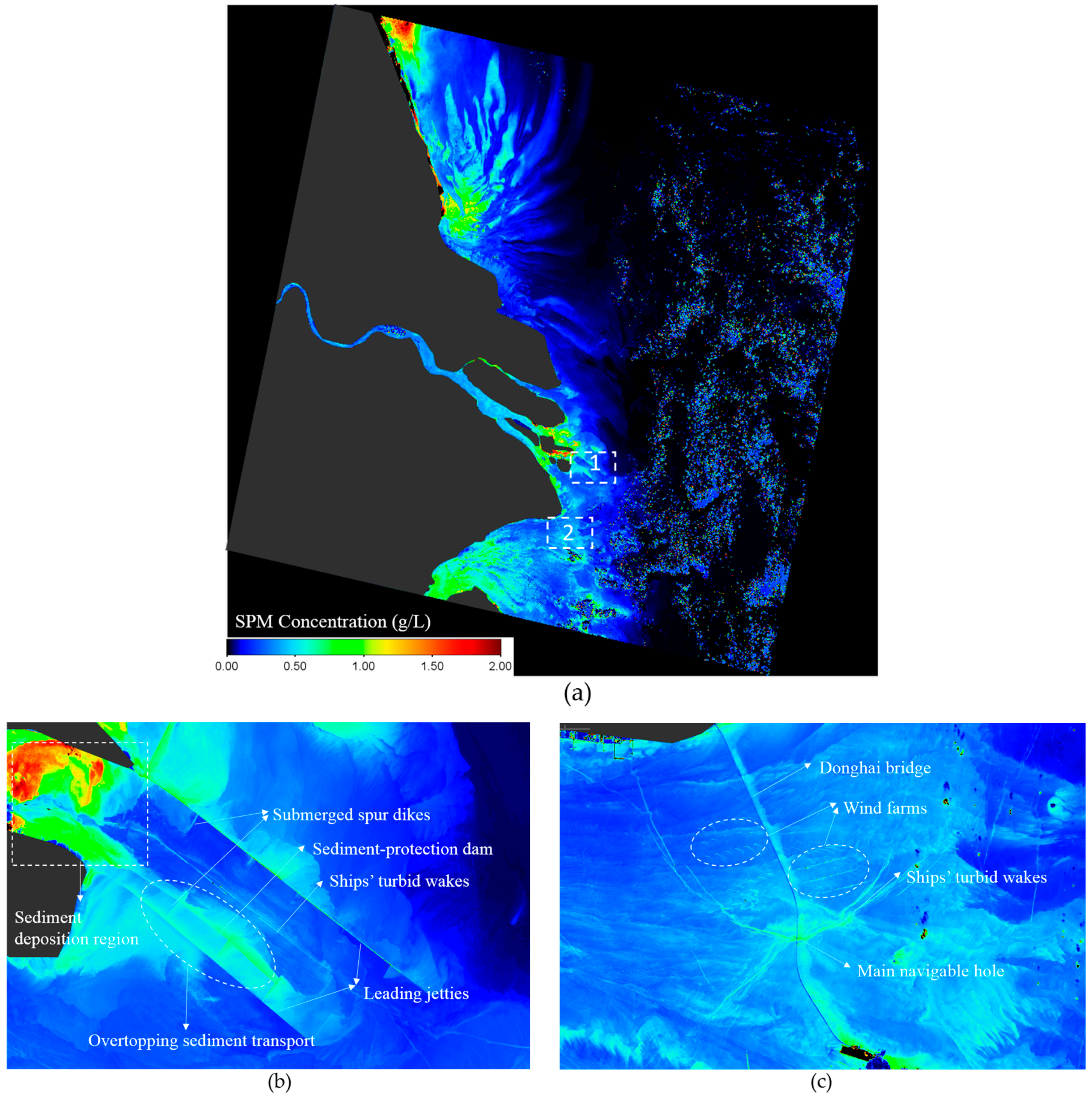
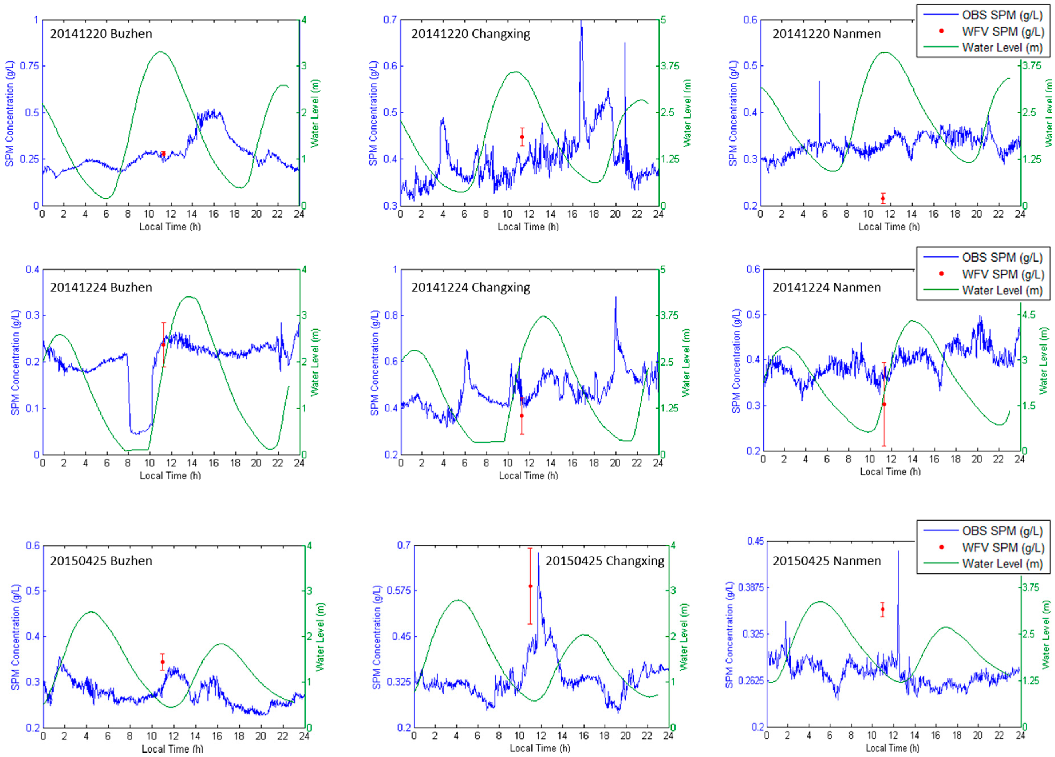
4.3. Quantitative Estimation of Suspended Particulate Matter and Validation
5. Conclusions
Acknowledgments
Author Contributions
Conflicts of Interest
References
- Schoellhamer, D.H.; Mumley, T.E.; Leatherbarrow, J.E. Suspended sediment and sediment-associated contaminants in San Francisco Bay. Environ. Res. 2007, 105, 119–131. [Google Scholar] [CrossRef] [PubMed]
- El-Asmar, H.M.; White, K. Changes in coastal sediment transport processes due to construction of New Damietta Harbour, Nile Delta, Egypt. Coast. Eng. 2002, 46, 127–138. [Google Scholar] [CrossRef]
- Chen, S.; Zhang, G.; Yang, S. Temporal and spatial changes of suspended sediment concentration and resuspension in the Yangtze River estuary. J. Geogr. Sci. 2003, 13, 498–506. [Google Scholar]
- Vanhellemont, Q.; Neukermans, G.; Ruddick, K. Synergy between polar-orbiting and geostationary sensors: Remote sensing of the ocean at high spatial and high temporal resolution. Remote Sens. Environ. 2014, 146, 49–62. [Google Scholar] [CrossRef]
- Vanhellemont, Q.; Ruddick, K. Turbid wakes associated with offshore wind turbines observed with Landsat 8. Remote Sens. Environ. 2014, 145, 105–115. [Google Scholar] [CrossRef]
- IOCCG Atmospheric Correction for Remotely-Sensed Ocean-Colour Products. Available online: http://www.star.nesdis.noaa.gov/sod/mecb/color/documents/IOCCG_report_10.pdf (accessed on 2 May 2016).
- Gordon, H.R.; Wang, M. Retrieval of water-leaving radiance and aerosol optical thickness over the oceans with SeaWiFS: A preliminary algorithm. Appl. Opt. 1994, 33, 443–452. [Google Scholar] [CrossRef] [PubMed]
- Ruddick, K.; Ovidio, F.; Rijkeboer, M. Atmospheric correction of SeaWiFS imagery for turbid coastal and inland waters. Appl. Opt. 2000, 39, 897–912. [Google Scholar] [CrossRef] [PubMed]
- Wang, M.; Wei, S. Estimation of ocean contribution at the MODIS near-infrared wavelengths along the east coast of the US: Two case studies. Geophys. Res. Lett. 2005. [Google Scholar] [CrossRef]
- Vanhellemont, Q.; Ruddick, K. Advantages of high quality SWIR bands for ocean colour processing: Examples from Landsat-8. Remote Sens. Environ. 2015, 161, 89–106. [Google Scholar] [CrossRef]
- Li, Z.F. Application of GF-1 Satellite in Land-use Remote Sensing Monitoring. Land Resour. Herald 2015, 12, 85–88. [Google Scholar]
- Wu, P.Q.; Zhang, J.; Ma, Y. Positioning Precision Evaluation of GF-1 in the Coastal Zone. Hydrogr. Surv. Chart. 2015, 35, 63–66. [Google Scholar]
- Zhang, K.; Ma, S.B.; Li, Z.R.; Liu, S.Y. Geological Interpretation of GF-1 Satellite Imagery. Remote Sens. Inf. 2016, 31, 115–123. [Google Scholar]
- Li, F.L.; Wang, L.; Liu, J.; Chang, Q.R. Remote Sensing Estimation of SPAD Value for Wheat Leaf Based on GF-1 Data. Trans. Chin. Soc. Agric. Mach. 2015, 46, 273–281. [Google Scholar]
- Liang, W.X.; Li, J.S.; Zhou, D.M.; Shen, Q.; Zhang, F.F. Evaluation of GF-1 WFV Characteristics in Monitoring Inland Water Environment. Remote Sens. Technol. Appl. 2015, 30, 810–818. [Google Scholar]
- Cheng, Q.; Liu, B.; Li, T.; Zhu, L. Research on remote sensing retrieval of suspended sediment concentration in Hangzhou Bay by GF-1 satellite. Mar. Environ. Sci. 2015, 34, 558–563. [Google Scholar]
- Zhu, L.; Li, Y.M.; Zhao, S.H.; Guo, Y.L. Remote sensing monitoring of Taihu Lake water quality by using GF-1 WFV data. Remote Sens. Land Resour. 2015, 27, 113–120. [Google Scholar]
- He, Q.; Yun, C.X.; Shi, W.R. Remote sensing analysis for suspended sediment concentration in water surface layer in Yangtze River estuary. Prog. Nat. Sci. 1999, 9, 160–164. [Google Scholar]
- Bai, Z.G. The technical feature of GF-1 satellite. Aerosp. China 2013, 8, 5–9. [Google Scholar]
- Irons, J.R.; Dwyer, J.L.; Barsi, J.A. The next Landsat satellite: The Landsat Data Continuity Mission. Remote Sens. Environ. 2012, 122, 11–21. [Google Scholar] [CrossRef]
- Zhu, B.; Wang, X.H.; Tang, L.L.; Li, C.R. Review on Methods for SNR Estimation of Optical Remote Sensing Imagery. Remote Sens. Technol. Appl. 2010, 25, 303–309. [Google Scholar]
- CRESDA Absolute Radiometric Calibration Coefficient. Available online: http://www.cresda.com/CN/Downloads/dbcs/6709.shtml (accessed on 2 May 2016).
- RBINS ACOLITE. Available online: http://odnature.naturalsciences.be/remsem/software-and-data/acolite (accessed on 2 May 2016).
- Mueller, J.L.; Fargion, G.S.; Mcclain, C.R.; Pietras, C.; Hooker, S.B.; Austin, R.W.; Miller, M.; Knobelspiesse, K.D.; Frouin, R.; Holben, B. Ocean Optics Protocols For Satellite Ocean Color Sensor Validation, Revision 4, Volume II: Instrument Specifications, Characterization and Calibration. Available online: https://ntrs.nasa.gov/archive/nasa/casi.ntrs.nasa.gov/20020044096.pdf (accessed on 2 May 2016).
- Leonid, G.S.; Shen, F. Optical closure for remote-sensing reflectance based on accurate radiative transfer approximations: The case of the Changjiang (Yangtze) River Estuary and its adjacent coastal area, China. Int. J. Remote Sens. 2014, 35, 4193–4224. [Google Scholar]
- Shen, F.; Verhoef, W.; Zhou, Y.; Salama, M.S.; Liu, X. Satellite Estimates of Wide-Range Suspended Sediment Concentrations in Changjiang (Yangtze) Estuary Using MERIS Data. Estuar. Coasts 2010, 33, 1420–1429. [Google Scholar] [CrossRef]
- Shen, F.; Zhou, Y.; Peng, X.; Chen, Y. Satellite multi-sensor mapping of suspended particulate matter in turbid estuarine and coastal ocean, China. Int. J. Remote Sens. 2014, 35, 4173–4192. [Google Scholar] [CrossRef]
- Kubelka, P.; Munk, F. Ein beitrag zur optik der farbanstriche. Z. Tech. Phys. 1931, 12, 593–601. [Google Scholar]
- Shen, F.; Zhou, Y.; Li, J.; He, Q.; Verhoef, W. Remotely sensed variability of the suspended sediment concentration and its response to decreased river discharge in the Yangtze estuary and adjacent coast. Cont. Shelf Res. 2013, 69, 52–61. [Google Scholar] [CrossRef]
- Gordon, H.R.; Brown, O.B.; Jacobs, M.M. Computed Relationships between the Inherent and Apparent Optical Properties of a Flat Homogeneous Ocean. Appl. Opt. 1975, 14, 417–427. [Google Scholar] [CrossRef] [PubMed]
- Vermote, E.F.; Tanre, D.; Deuze, J.L.; Herman, M.; Morcrette, J.J. Second simulation of a satellite signal in the solar spectrum-vector (6SV). In Proceedings of the Geoscience and Remote Sensing Symposium, 1990 (IGARSS’90) ‘Remote Sensing Science for the Nineties’, 10th Annual International, Washington, DC, USA, 20–24 May 1990.
- Xue, Y.Z.; He, Q.; Wang, Y.Y. The method and application of OBS in the measurement of sediment concentration. J. Sediment Res. 2004, 4, 56–60. [Google Scholar]


| Band ID | Band Range (nm) | SNR | F0 (W m−2·μm−1) | |||
|---|---|---|---|---|---|---|
| GF-1/WFV | L-8/OLI | GF-1/WFV | L-8/OLI | GF-1/WFV | L-8/OLI | |
| 1 (Coastal/aerosol) | - | 433–453 | - | - | - | 1895.6 |
| 2 (Blue) | 450–520 | 450–515 | 78.127 | 122.798 | 1966.8 | 2004.6 |
| 3 (Green) | 520–590 | 525–600 | 52.672 | 96.358 | 1822.6 | 1820.7 |
| 4 (Red) | 630–690 | 630–680 | 40.815 | 111.941 | 1523.2 | 1549.4 |
| 5 (NIR) | 770–890 | 845–885 | 34.610 | 92.315 | 1066.5 | 951.2 |
| 6 (SWIR1) | - | 1560–1660 | - | - | - | 247.6 |
| 7 (SWIR2) | - | 2100–2300 | - | - | - | 85.5 |
| 8 (PAN) | - | 500–680 | - | - | - | 1724.0 |
| 9 (CIRRUS) | - | 1360–1390 | - | - | - | 367.0 |
| Aquired Date | GF-1/WFV | Landsat-8/OLI | |||||
|---|---|---|---|---|---|---|---|
| Sensor | Center Lat (°) | Center Lon (°) | Center Time (GMT) | Center Lat (°) | Center Lon (°) | Center Time (GMT) | |
| 4 November 2014 | WFV1 | N31.3 | E120.8 | 02:56:54 | N31.6 | E121.9 | 02:25:13 |
| WFV1 | N33.0 | E121.2 | 02:56:26 | ||||
| WFV2 | N31.0 | E122.9 | 02:56:54 | N30.3 | E121.5 | 02:25:36 | |
| WFV2 | N32.6 | E123.3 | 02:56:26 | ||||
| 20 December 2014 | WFV4 | N31.8 | E121.8 | 03:19:16 | |||
| 24 December 2014 | WFV4 | N31.9 | E121.8 | 03:17:04 | |||
| 25 April 2015 | WFV1 | N31.3 | E121.7 | 02:56:36 | |||
| Sensor | Band ID | α | β | APD (%) | RMSE (sr−1) | R2 (%) |
|---|---|---|---|---|---|---|
| WFV | Band 1 (blue) | 0.0329 | 78.33 | 26.7 | 0.0048 | 60.7 |
| WFV | Band 2 (green) | 0.0530 | 47.94 | 27.6 | 0.0067 | 70.8 |
| WFV | Band 3 (red) | 0.0746 | 18.32 | 42.4 | 0.0082 | 77.9 |
| WFV | Band 4 (NIR) | 0.0935 | 4.066 | 53.1 | 0.0058 | 87.2 |
| Model | Parameter Name | Data Range | Step |
|---|---|---|---|
| 6S | Solar zenith angle | 0°~70° | 5° |
| Sensor zenith angle | 0°~70° | 5° | |
| Scattering angle | 0°~180° | 45° | |
| Scene aquired date (Julian day) | 1~365 | 60 | |
| Atmospheric model | Midlatitude summer | - | |
| Midlatitude winter | |||
| Aerosol type | Continental | - | |
| Maritime | |||
| Urban | |||
| Aerosol optical depth at 550 nm | 0.05–2.00 | 0.05 | |
| WFV band | 1–4 | 1 | |
| SERT | SPM concentration | 0.001 g/L~10 g/L (N = 100 in log-scale) | |
© 2016 by the authors; licensee MDPI, Basel, Switzerland. This article is an open access article distributed under the terms and conditions of the Creative Commons Attribution (CC-BY) license (http://creativecommons.org/licenses/by/4.0/).
Share and Cite
Shang, P.; Shen, F. Atmospheric Correction of Satellite GF-1/WFV Imagery and Quantitative Estimation of Suspended Particulate Matter in the Yangtze Estuary. Sensors 2016, 16, 1997. https://doi.org/10.3390/s16121997
Shang P, Shen F. Atmospheric Correction of Satellite GF-1/WFV Imagery and Quantitative Estimation of Suspended Particulate Matter in the Yangtze Estuary. Sensors. 2016; 16(12):1997. https://doi.org/10.3390/s16121997
Chicago/Turabian StyleShang, Pei, and Fang Shen. 2016. "Atmospheric Correction of Satellite GF-1/WFV Imagery and Quantitative Estimation of Suspended Particulate Matter in the Yangtze Estuary" Sensors 16, no. 12: 1997. https://doi.org/10.3390/s16121997