
Image Based Mango Fruit Detection, Localisation and Yield Estimation Using Multiple View Geometry


Abstract
:1. Introduction
2. Materials and Methods
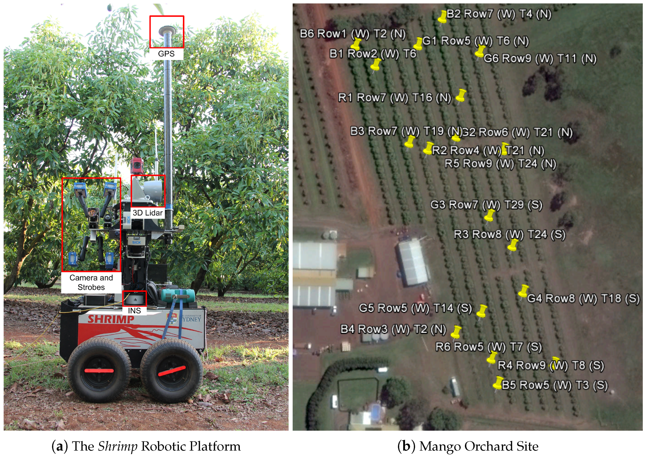
2.1. Data Collection
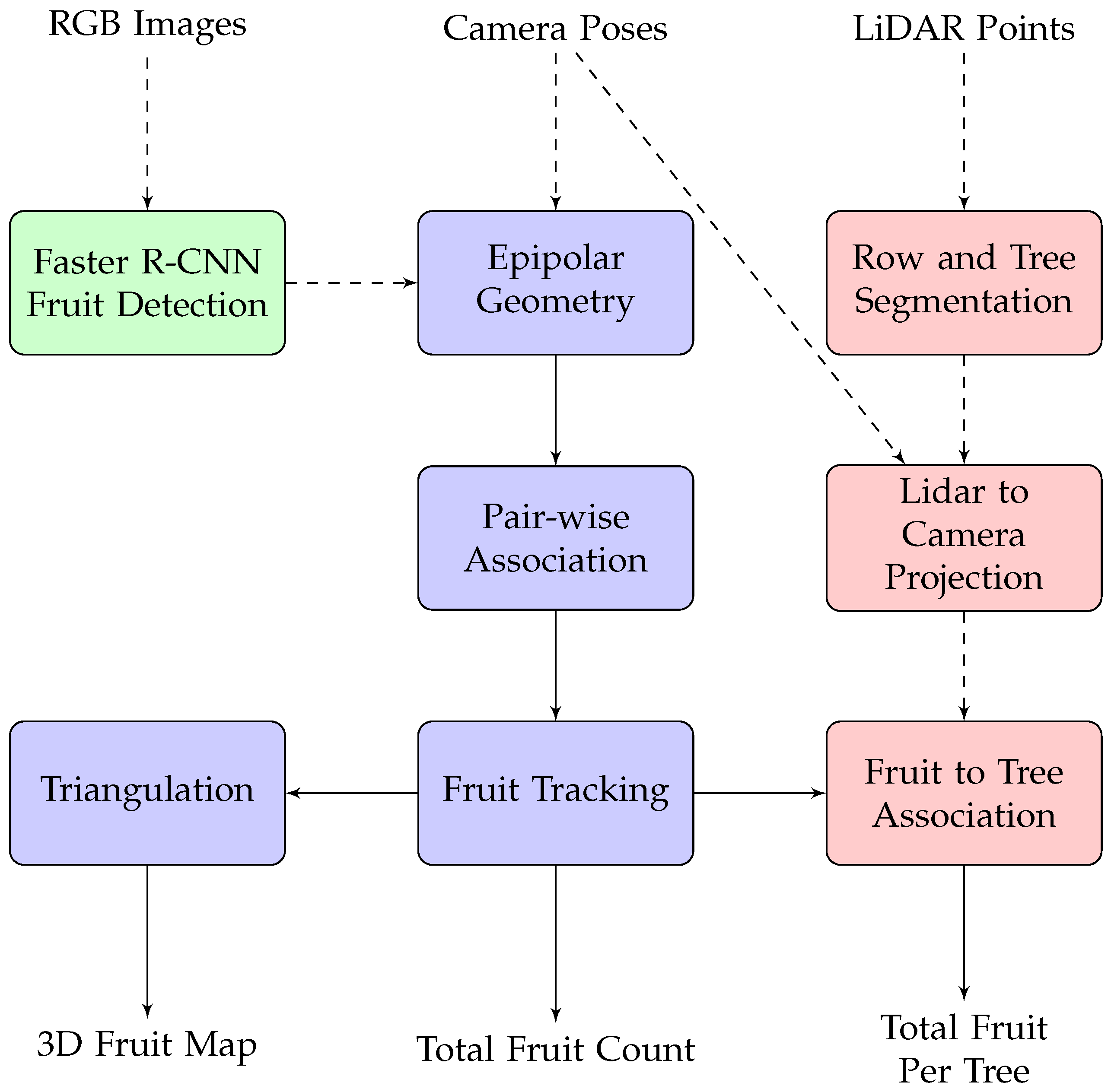
2.2. Fruit Detection
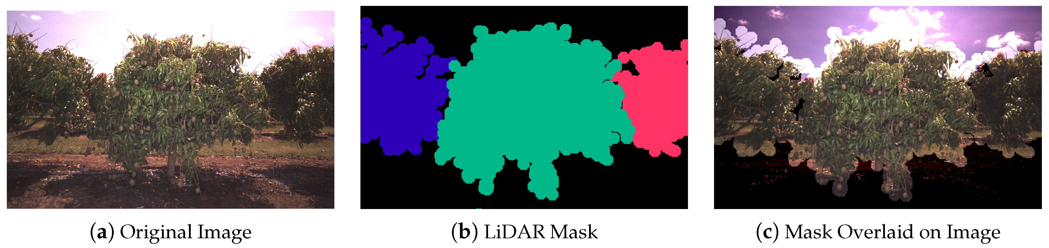
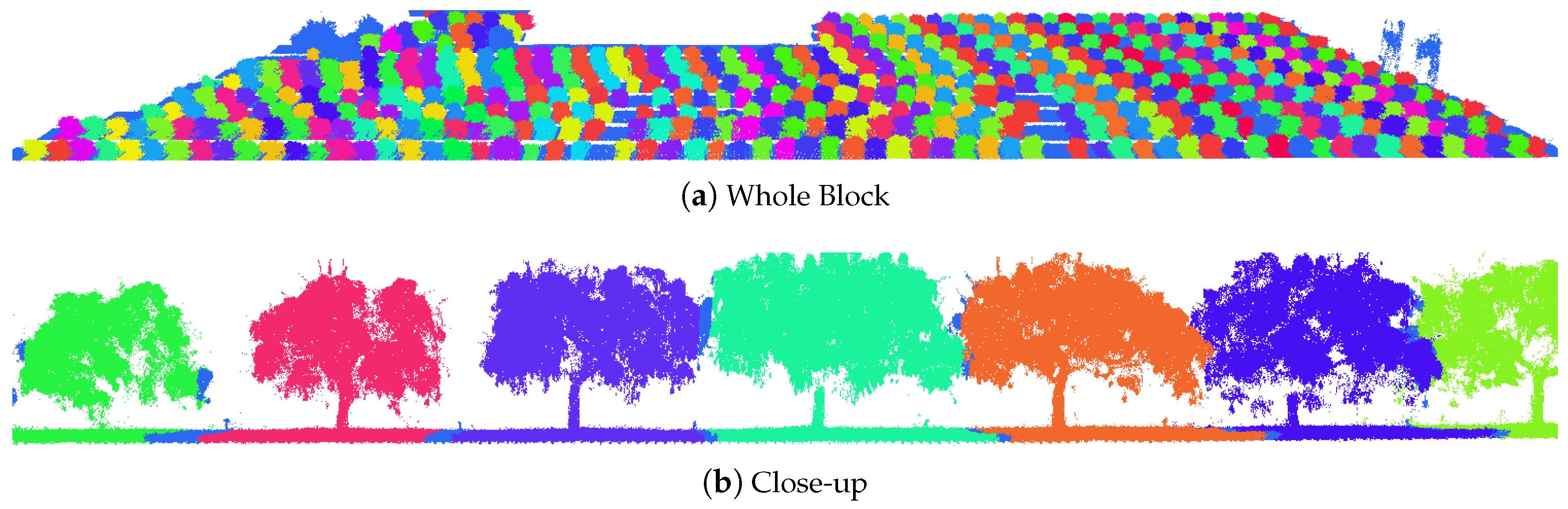
2.3. Tree Segmentation
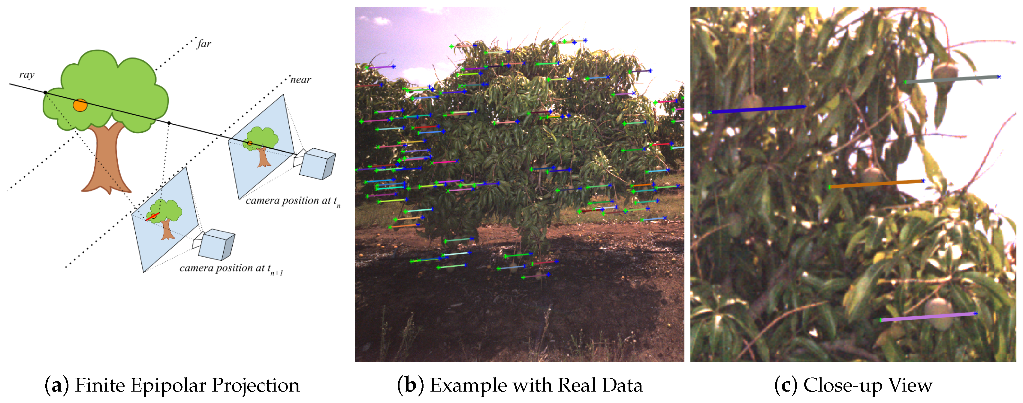
2.4. Fruit Tracking, Localisation and Counting
3. Results
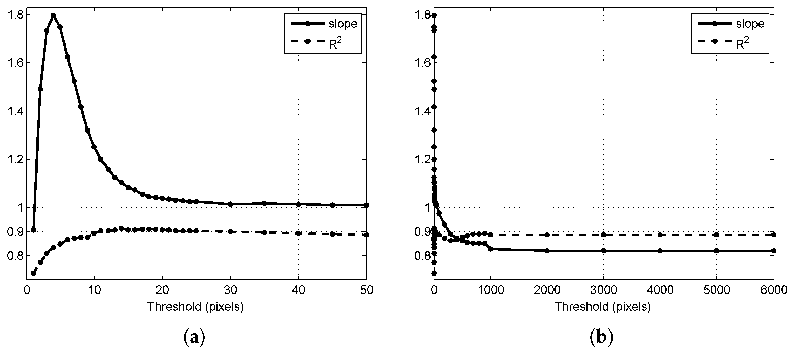
3.1. Threshold Selection
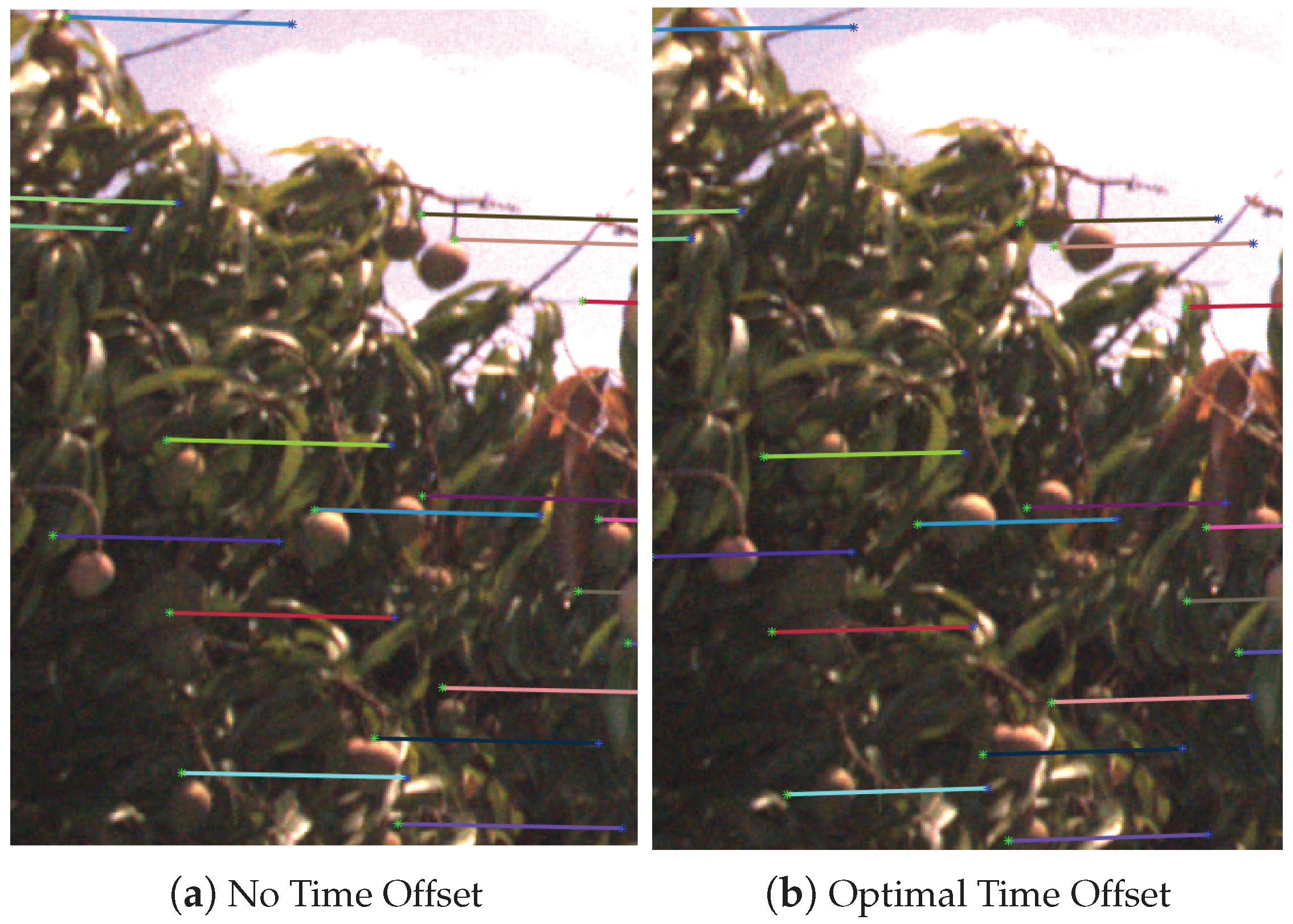
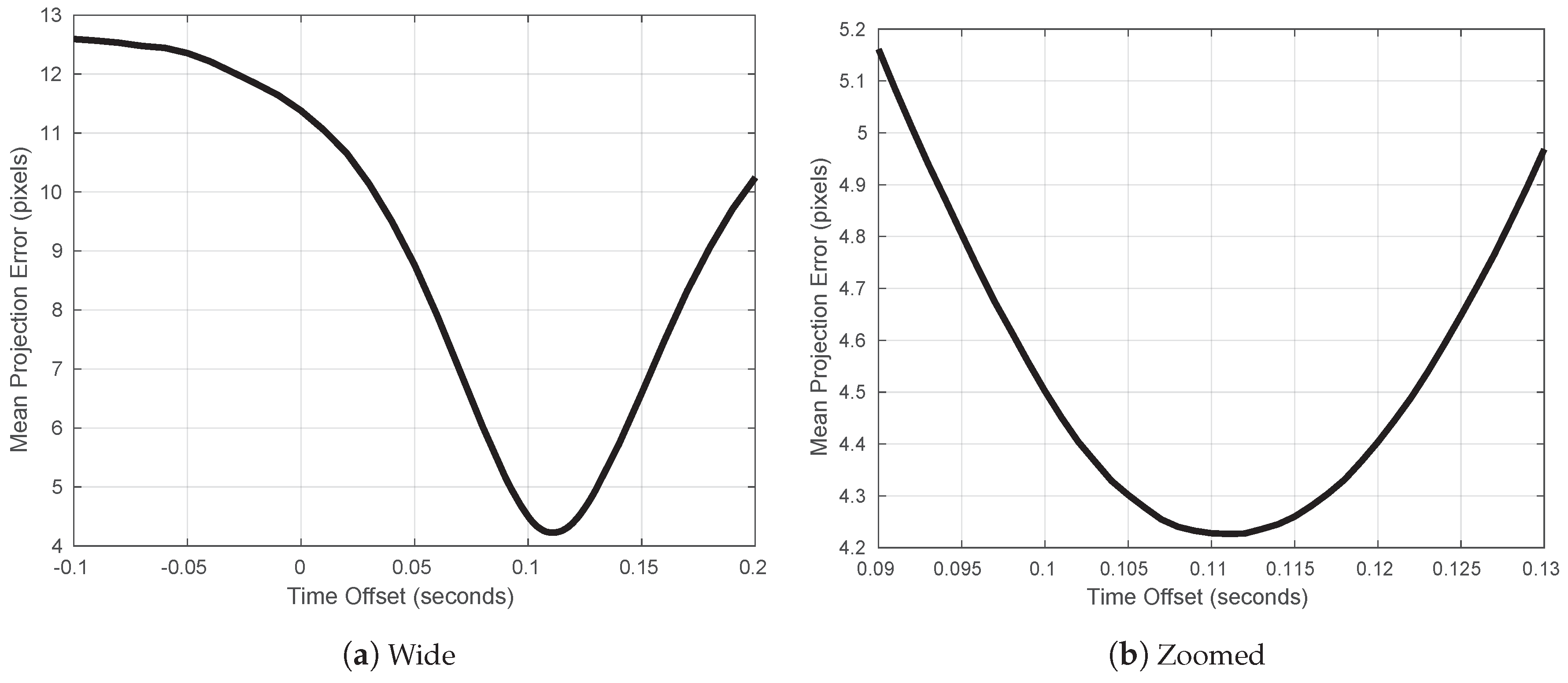
3.2. Camera and Navigation Timestamp Offset Correction
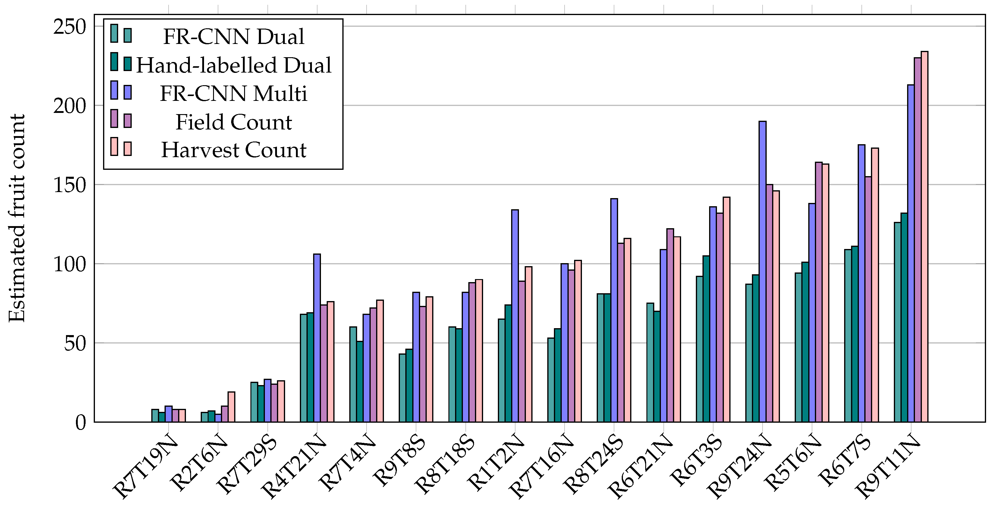
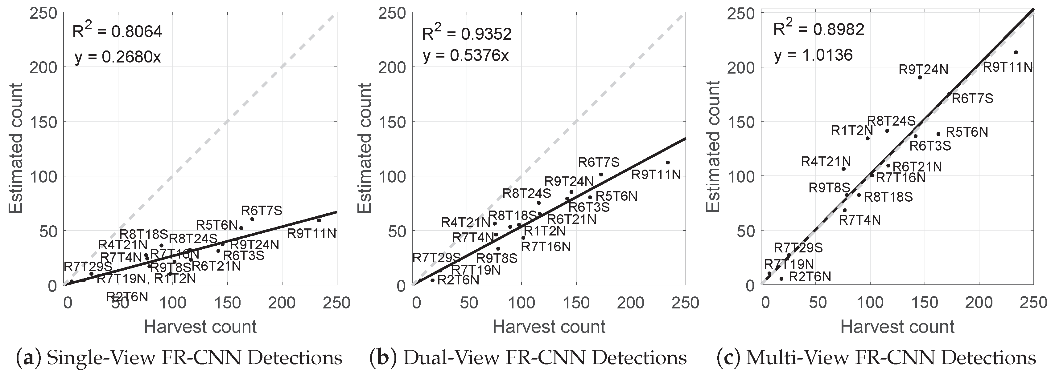
3.3. Fruit Counts
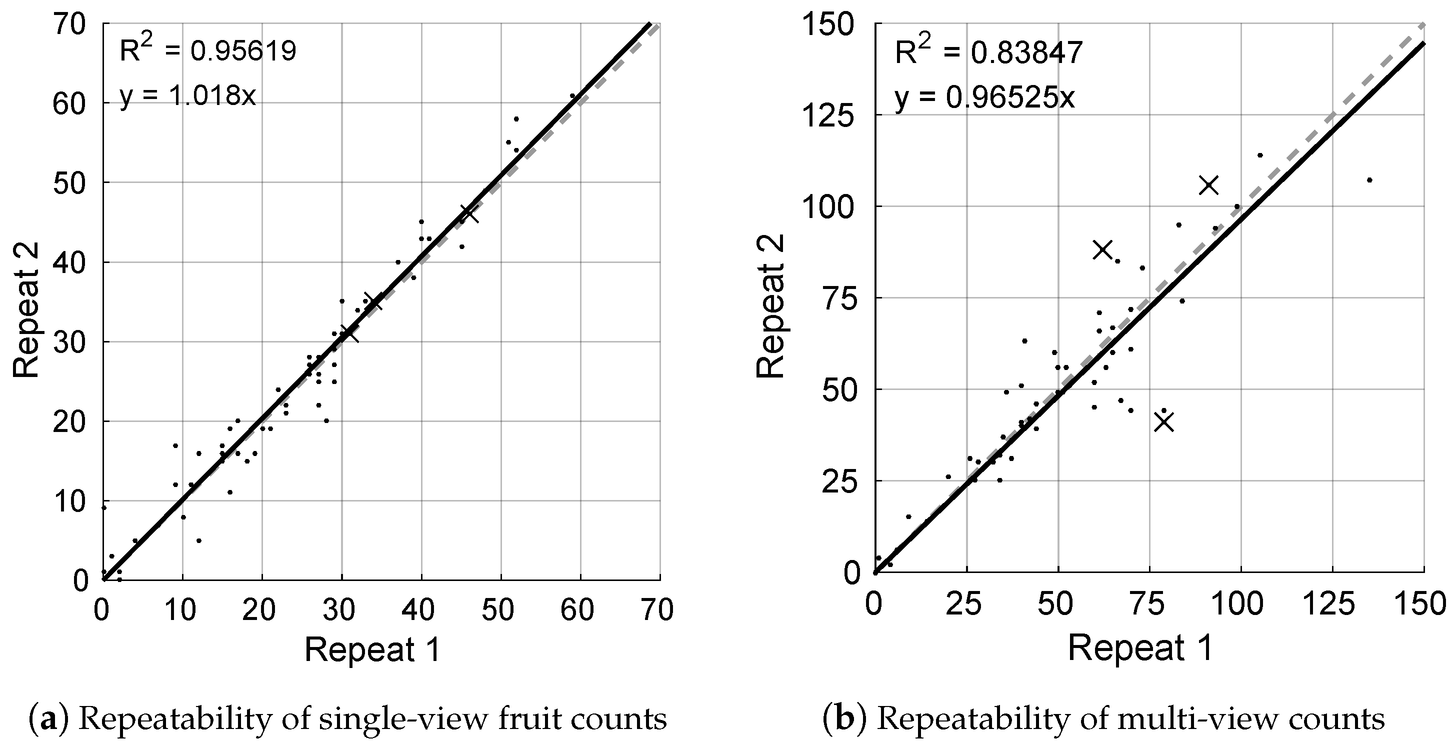
3.4. Repeatability
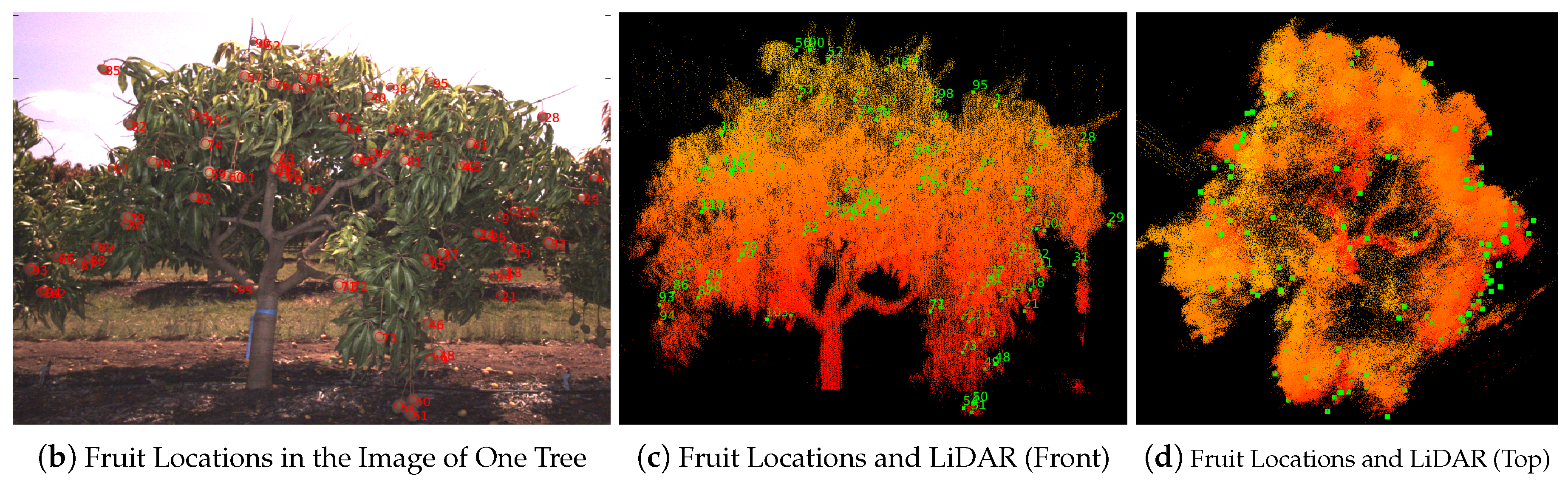
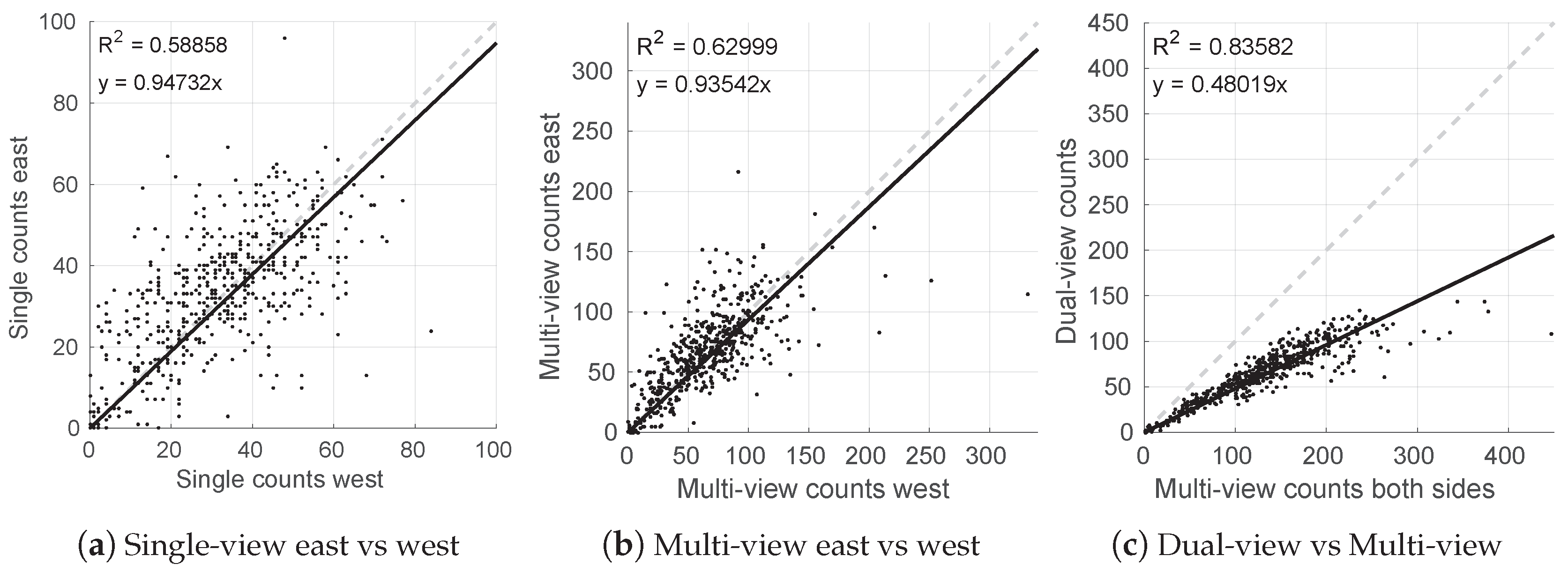
3.5. Triangulation
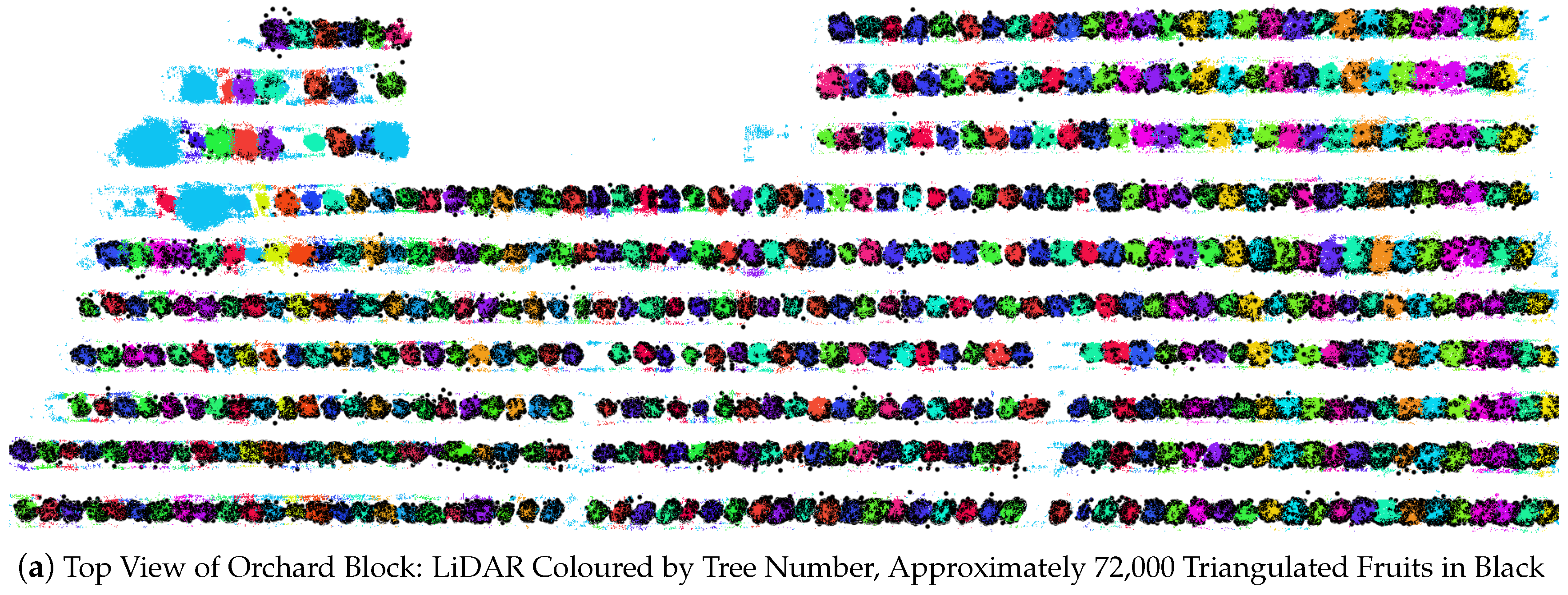
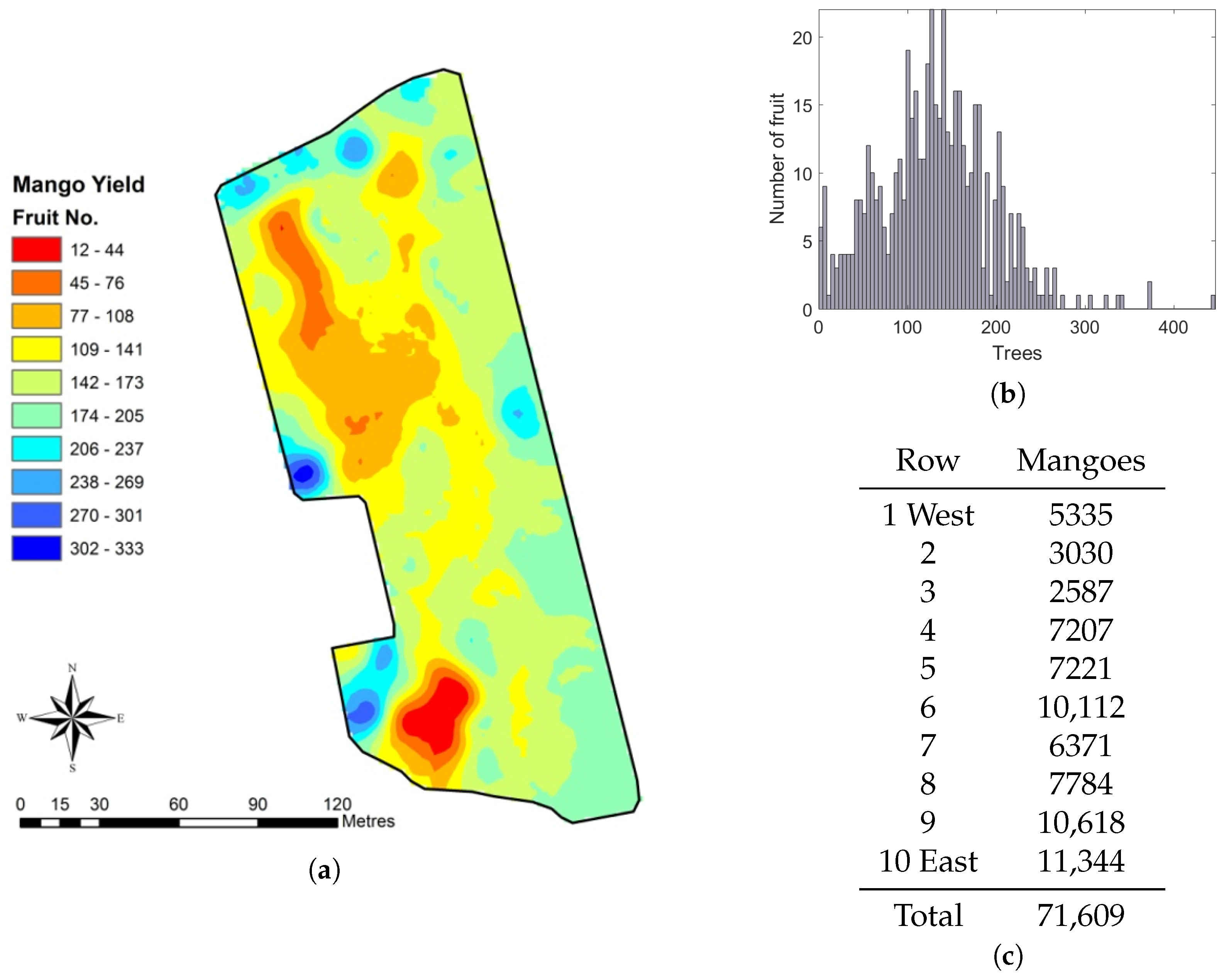
3.6. Orchard Statistics
- Spatial fruit-yield map
- Fruit totals per tree, row and block
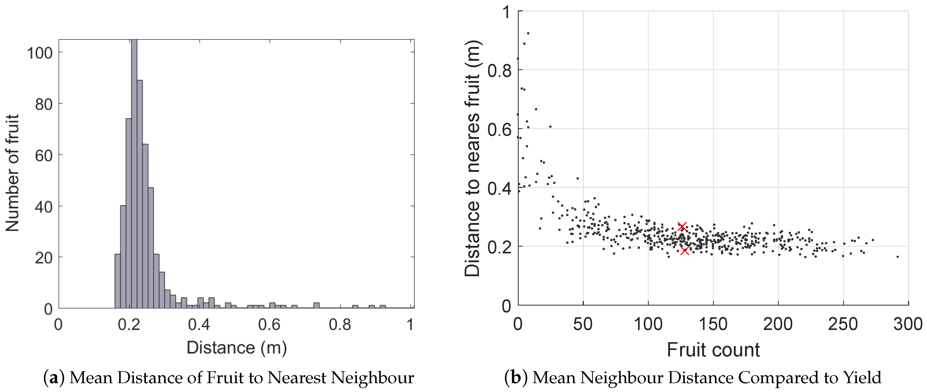
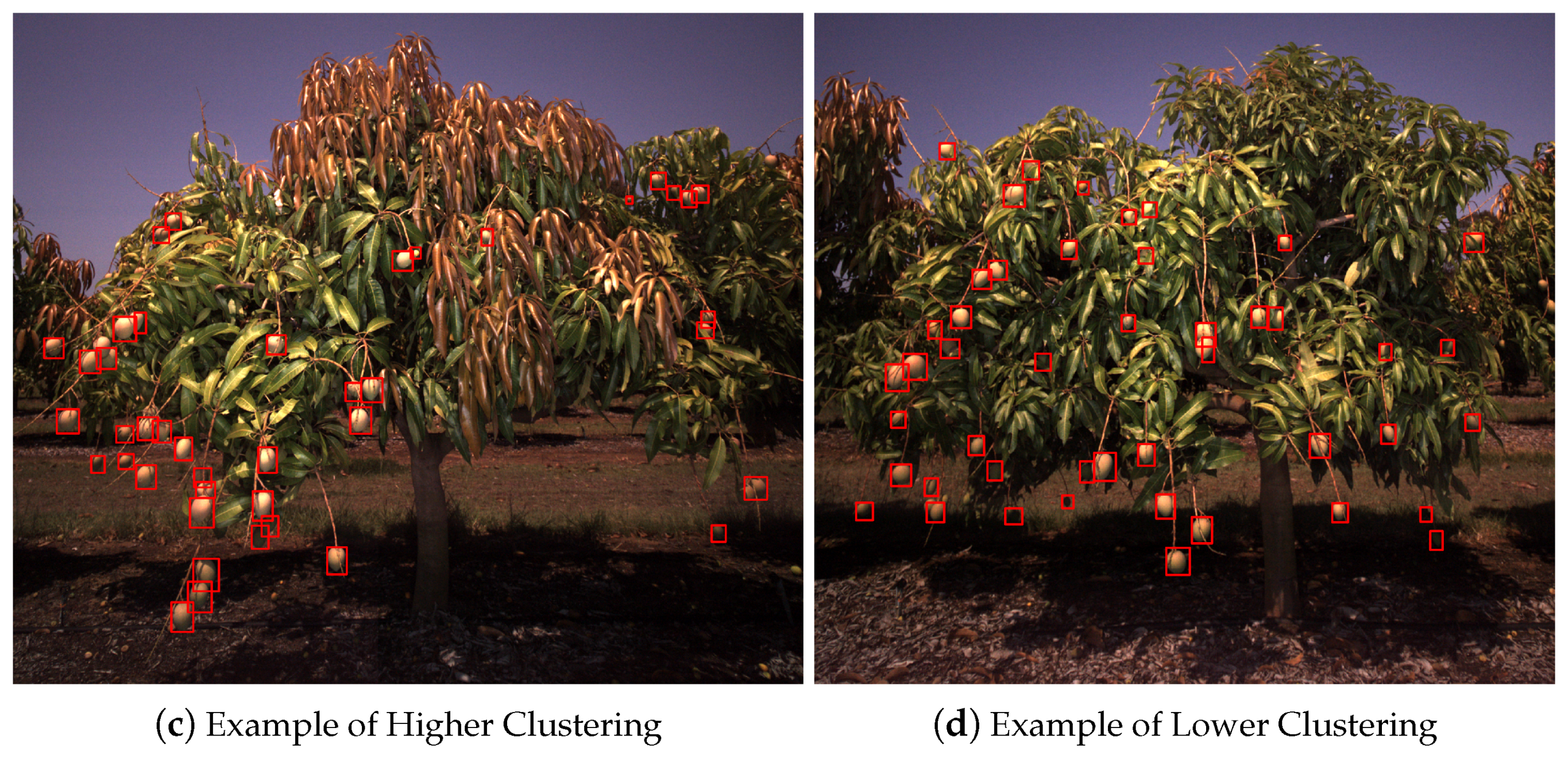
- Histograms of fruit clustering (are the fruits evenly distributed within the canopy or not?)
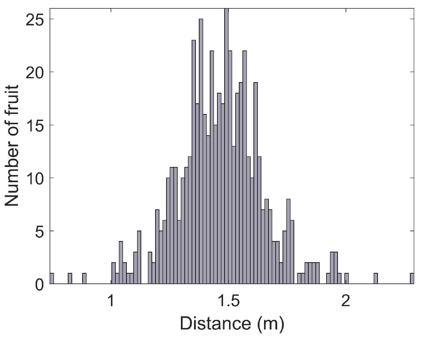
- Histograms of fruit heights above the ground
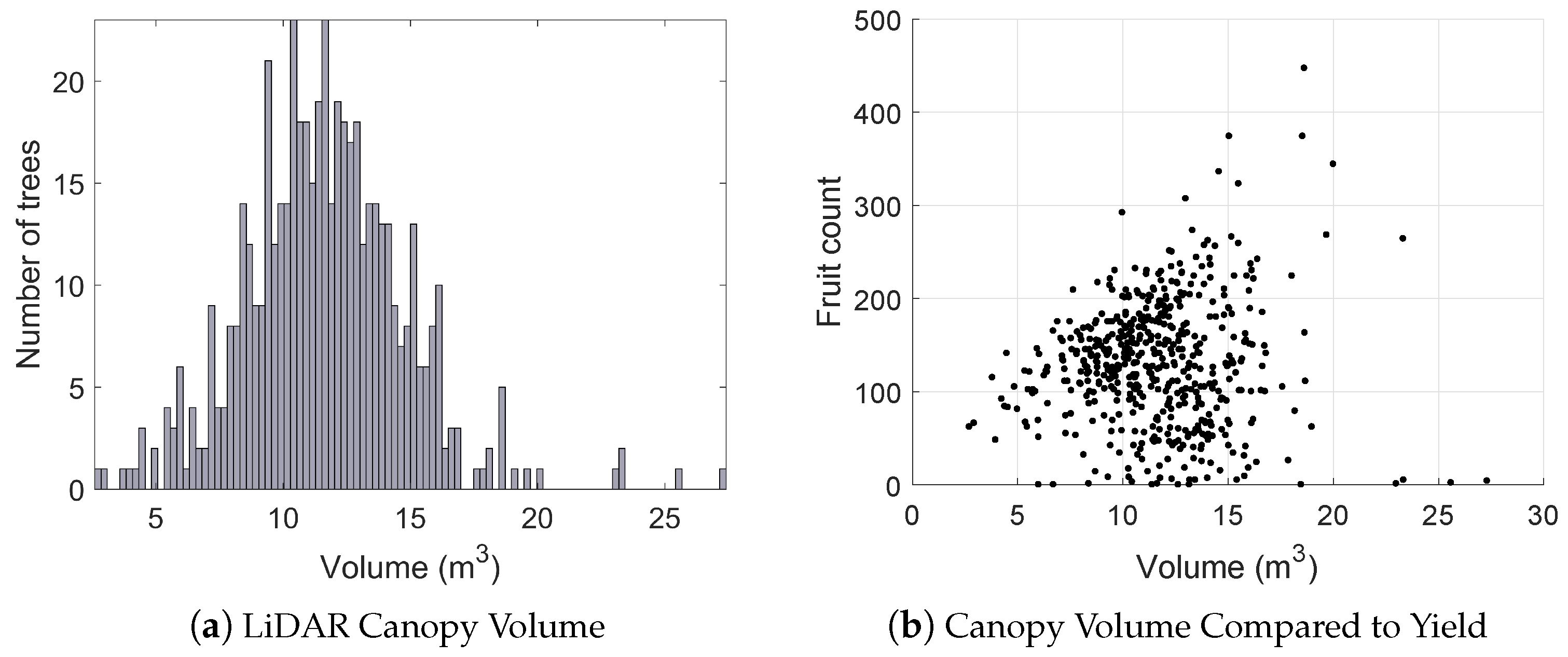
- Histograms of canopy volume and relationship to yield
4. Discussion
4.1. Performance of the Single, Dual and Multi-View Methods
4.2. Multiple Views as a Solution to Occlusion
4.3. The Benefits of LiDAR
4.4. Problem Cases
4.4.1. Missing Frames and Platform Oscillation
4.4.2. Track Fragmentation and Over-Counting
4.4.3. Fruit Bunching and Ambiguous Track Association
4.4.4. Ground Extraction from LiDAR Masks and Counting Fallen Fruit
5. Conclusions
Acknowledgments
Author Contributions
Conflicts of Interest
References
- Payne, A.B.; Walsh, K.B.; Subedi, P.P.; Jarvis, D. Estimation of mango crop yield using image analysis–segmentation method. Comput. Electron. Agric. 2013, 91, 57–64. [Google Scholar] [CrossRef]
- Jimenez, A.R.; Ceres, R.; Pons, J.L. A survey of computer vision methods for locating fruit on trees. Trans. Am. Soc. Agric. Eng. 2000, 43, 1911–1920. [Google Scholar] [CrossRef]
- Gongal, A.; Amatya, S.; Karkee, M.; Zhang, Q.; Lewis, K. Sensors and systems for fruit detection and localization: A review. Comput. Electron. Agric. 2015, 116, 8–19. [Google Scholar] [CrossRef]
- Wang, Q.; Nuske, S.; Bergerman, M.; Singh, S. Automated Crop Yield Estimation for Apple Orchards. In Experimental Robotics; Springer: Berlin, Germany, 2013; pp. 745–758. [Google Scholar]
- Hung, C.; Underwood, J.; Nieto, J.; Sukkarieh, S. A Feature Learning Based Approach for Automated Fruit Yield Estimation. In Field and Service Robotics: Results of the 9th International Conference; Mejias, L., Corke, P., Roberts, J., Eds.; Springer: Berlin, Germany, 2015; pp. 485–498. [Google Scholar]
- Bargoti, S.; Underwood, J. Image classification with orchard metadata. In Proceedings of the International Conference on Robotics and Automation (ICRA), Stockholm, Sweden, 16–21 May 2016; pp. 5164–5170.
- Underwood, J.P.; Hung, C.; Whelan, B.; Sukkarieh, S. Mapping almond orchard canopy volume, flowers, fruit and yield using LiDAR and vision sensors. Comput. Electron. Agric. 2016, 130, 83–96. [Google Scholar] [CrossRef]
- Cheein, F.A.A.; Carelli, R. Agricultural robotics: Unmanned robotic service units in agricultural tasks. IEEE Ind. Electron. Mag. 2013, 7, 48–58. [Google Scholar] [CrossRef]
- Das, J.; Cross, G.; Qu, C.; Makineni, A.; Tokekar, P.; Mulgaonkar, Y.; Kumar, V. Devices, systems, and methods for automated monitoring enabling precision agriculture. In Proceedings of the International Conference on Autonomation and Science and Engineering, Gothenburg, Sweden, 24–28 August 2015; pp. 462–469.
- Hung, C.; Nieto, J.; Taylor, Z.; Underwood, J.; Sukkarieh, S. Orchard fruit segmentation using multi-spectral feature learning. In Proceedings of the International Conference on Intelligent Robots and Systems (IROS), Tokyo, Japan, 3–7 November 2013; pp. 5314–5320.
- Payne, A.; Walsh, K. Machine vision in estimation of fruit crop yield. In Plant Image Analysis: Fundamentals and Applications; CRC Press: New York, NY, USA, 2014; p. 329. [Google Scholar]
- Qureshi, W.; Payne, A.; Walsh, K.; Linker, R.; Cohen, O.; Dailey, M. Machine vision for counting fruit on mango tree canopies. Precis. Agric. 2016. [Google Scholar] [CrossRef]
- Stajnko, D.; Lakota, M.; Hočevar, M. Estimation of number and diameter of apple fruits in an orchard during the growing season by thermal imaging. Comput. Electron. Agric. 2004, 42, 31–42. [Google Scholar] [CrossRef]
- Linker, R.; Cohen, O.; Naor, A. Determination of the number of green apples in RGB images recorded in orchards. Comput. Electron. Agric. 2012, 81, 45–57. [Google Scholar] [CrossRef]
- Bargoti, S.; Underwood, J. Image Segmentation for Fruit Detection and Yield Estimation in Apple Orchards. J. Field Robot. 2016, in press. [Google Scholar]
- Bargoti, S.; Underwood, J. Deep Fruit Detection in Orchards. Available online: https://arxiv.org/abs/1610.03677 (accessed on 14 November 2016).
- Sa, I.; Ge, Z.; Dayoub, F.; Upcroft, B.; Perez, T.; McCool, C. DeepFruits: A Fruit Detection System Using Deep Neural Networks. Sensors 2016, 16, 1222. [Google Scholar] [CrossRef] [PubMed]
- Nuske, S.; Gupta, K.; Narasimhan, S.; Singh, S. Modeling and calibrating visual yield estimates in vineyards. In Field and Service Robotics; Springer: Berlin, Germany, 2014; pp. 343–356. [Google Scholar]
- Nuske, S.; Wilshusen, K.; Achar, S.; Yoder, L.; Narasimhan, S.; Singh, S. Automated visual yield estimation in vineyards. J. Field Robot. 2014, 31, 837–860. [Google Scholar] [CrossRef]
- Song, Y.; Glasbey, C.A.; Horgan, G.W.; Polder, G.; Dieleman, J.A.; van der Heijden, G.W.A.M. Automatic fruit recognition and counting from multiple images. Biosyst. Eng. 2014, 118, 203–215. [Google Scholar] [CrossRef]
- Moonrinta, J.; Chaivivatrakul, S.; Dailey, M.N.; Ekpanyapong, M. Fruit Detection, Tracking, and 3D Reconstruction for Crop Mapping and Yield Estimation. In Proceedings of the 11th International Conference on Control Automation Robotics & Vision (ICARCV), Singapore, 7–10 December 2010; pp. 1181–1186.
- Roy, P.; Stefas, N.; Peng, C.; Bayram, H.; Tokekar, P.; Isler, V. Robotic Surveying of Apple Orchards; TR 15-010; University of Minnesota, Computer Science and Engineering: Minneapolis, MN, USA, 2015. [Google Scholar]
- Kuhn, H.W. The Hungarian method for the assignment problem. Naval Res. Logist. Q. 1955, 2, 83–97. [Google Scholar] [CrossRef]
- Underwood, J.P.; Jagbrant, G.; Nieto, J.I.; Sukkarieh, S. LiDAR-based tree recognition and platform localization in orchards. J. Field Robot. 2015, 32, 1056–1074. [Google Scholar] [CrossRef]
- Ren, S.; He, K.; Girshick, R.B.; Sun, J. Faster R-CNN: Towards Real-Time Object Detection with Region Proposal Networks. Available online: https://arxiv.org/abs/1506.01497 (accessed on 14 November 2016).
- Allied Vision. Prosilica GT3300C. Available online: https://www.alliedvision.com/en/products/cameras/detail/ProsilicaGT/3300.html (accessed on 14 November 2016).
- Kowa. LM8CX. Available online: http://www.kowa-europe.com/lenses/en/LM8XC.30107.php (accessed on 14 November 2016).
- Excelitas. MVS-5002. Available online: http://www.excelitas.com/Lists/Industrial%20Lighting/DispForm.aspx?ID=14 (accessed on 14 November 2016).
- Velodyne. HDL64E. Available online: http://velodynelidar.com/hdl-64e.html (accessed on 14 November 2016).
- Novatel. IMU-CPT. Available online: http://www.novatel.com/products/span-gnss-inertial-systems/span-imus/imu-cpt/ (accessed on 14 November 2016).
- The University of Sydney. Agricultural Robotics at the Australian Centre for Field Robotics. Available online: http://sydney.edu.au/acfr/agriculture (accessed on 14 November 2016).
- Simonyan, K.; Zisserman, A. Very Deep Convolutional Networks for Large-Scale Image Recognition. Available online: https://arxiv.org/abs/1409.1556 (accessed on 14 November 2016).
- Suchet Bargoti. Pychet Labeller. Available online: https://github.com/acfr/pychetlabeller (accessed on 14 November 2016).
- Wellington, C.; Campoy, J.; Khot, L.; Ehsani, R. Orchard tree modeling for advanced sprayer control and automatic tree inventory. In Proceedings of the IEEE/RSJ International Conference on Intelligent Robots and Systems (IROS) Workshop on Agricultural Robotics, Algarve, Portugal, 7–12 October 2012; pp. 5–6.
- Bargoti, S.; Underwood, J.P.; Nieto, J.I.; Sukkarieh, S. A Pipeline for Trunk Detection in Trellis Structured Apple Orchards. J. Field Robot. 2015, 32, 1075–1094. [Google Scholar] [CrossRef]
- Underwood, J.; Scheding, S.; Ramos, F. Real-time map building with uncertainty using colour camera and scanning laser. In Proceedings of the 2007 Australasian Conference on Robotics and Automation, Brisbane, Australia, 10–12 December 2007; pp. 1330–1334.
- Munkres, J. Algorithms for the assignment and transportation problems. J. Soc. Ind. Appl. Math. 1957, 5, 32–38. [Google Scholar] [CrossRef]
- Clapper, B.M. Munkres 1.0.8. Available online: https://pypi.python.org/pypi/munkres (accessed on 14 November 2016).
- Underwood, J.P.; Hill, A.; Peynot, T.; Scheding, S.J. Error modeling and calibration of exteroceptive sensors for accurate mapping applications. J. Field Robot. 2010, 27, 2–20. [Google Scholar] [CrossRef]


| Tree | r9t11n | r9t24n | r9t8s | r8t24s | r8t18s | r7t4n | r7t16n | r7t29s | r7t19n |
|---|---|---|---|---|---|---|---|---|---|
| Field count | 230 | 150 | 73 | 113 | 88 | 72 | 96 | 24 | 8 |
| Harvest count | 234 | 146 | 79 | 116 | 90 | 77 | 102 | 26 | 8 |
| Tree | r6t21n | r6t7s | r6t3s | r5t6n | r5t14s * | r4t21n | r3t2n * | r2t6n | r1t2n |
| Field count | 122 | 155 | 132 | 164 | 154 | 74 | 43 | 10 | 89 |
| Harvest count | 117 | 173 | 142 | 163 | 333 | 76 | 54 | 19 | 98 |
© 2016 by the authors; licensee MDPI, Basel, Switzerland. This article is an open access article distributed under the terms and conditions of the Creative Commons Attribution (CC-BY) license (http://creativecommons.org/licenses/by/4.0/).
Share and Cite
Stein, M.; Bargoti, S.; Underwood, J. Image Based Mango Fruit Detection, Localisation and Yield Estimation Using Multiple View Geometry. Sensors 2016, 16, 1915. https://doi.org/10.3390/s16111915
Stein M, Bargoti S, Underwood J. Image Based Mango Fruit Detection, Localisation and Yield Estimation Using Multiple View Geometry. Sensors. 2016; 16(11):1915. https://doi.org/10.3390/s16111915
Chicago/Turabian StyleStein, Madeleine, Suchet Bargoti, and James Underwood. 2016. "Image Based Mango Fruit Detection, Localisation and Yield Estimation Using Multiple View Geometry" Sensors 16, no. 11: 1915. https://doi.org/10.3390/s16111915
APA StyleStein, M., Bargoti, S., & Underwood, J. (2016). Image Based Mango Fruit Detection, Localisation and Yield Estimation Using Multiple View Geometry. Sensors, 16(11), 1915. https://doi.org/10.3390/s16111915