
A Combination of Genetic Algorithm and Particle Swarm Optimization for Vehicle Routing Problem with Time Windows


Abstract
:1. Introduction

| Algorithms | Remarks | ||
|---|---|---|---|
| The exact algorithms | Branch and bound method [4,5] | The Efficiency depends on the depth of the branch and bound tree. | |
| Set segmentation method [6,7] | Hard to determine the minimum cost for each solutions. | ||
| Dynamic programming method [8,9] | Effective to limited-size problems, hard to consider the concrete demands such as time windows. | ||
| Integer programming algorithm [10,11] | High precision, time consuming, complex. | ||
| The heuristic algorithms | The traditional heuristic algorithms | Savings algorithm [12,13] | Computes rapidly, hard to get the optimal solution. |
| Sweep algorithm [14,15] | Suitable to the same number of customers for each route with few routes. | ||
| Two-phase algorithm [16,17] | Hard to get the optimal solution. | ||
| The meta-heuristic algorithms | Tabu search algorithm [18,19,20] | Has the good ability of local search, but is time consuming, and depends on the initial solution. | |
| Genetic algorithm [13,21] | Has the good ability of global search, computes rapidly, hard to obtain the global optimal solution. | ||
| Iterated local search [22,23] | Has the strength of fast convergence rate and low computational complexity. | ||
| Simulated annealing algorithm [24,25] | Slow convergence rates, carefully chosen tunable parameters. | ||
| Variable neighborhood Search [26,27] | Is suitable for large and complex optimization problems with constraints. | ||
| Ant colony algorithm [28,29,30] | Has good positive feedback mechanism, but is time consuming and prone to stagnation. | ||
| Neural network algorithm [31,32] | Computes rapidly, has slow convergence and can easily be trapped in a local optimum | ||
| Artificial bee colony algorithm [30,33] | Achieves a fast convergence speed, is associated with the piecewise linear cost approximation. | ||
| Particle swarm optimization [34,35,36] | Is robust and has fast searching speed, brings easily premature convergence. | ||
| Hybrid algorithm [2,8,12,20,28,37,38] | Is simple with fast optimizing speed and less calculation. | ||
2. Vehicle Routing Problem with Time Windows (VRPTW)
3. Particle Swarm Optimization (PSO)
4. The Proposed Algorithm
4.1. Particle Encoding
4.2. Inertia Weight Function
4.3. Crossover Operator of Genetic Algorithm
4.4. The Proposed Algorithm Flow
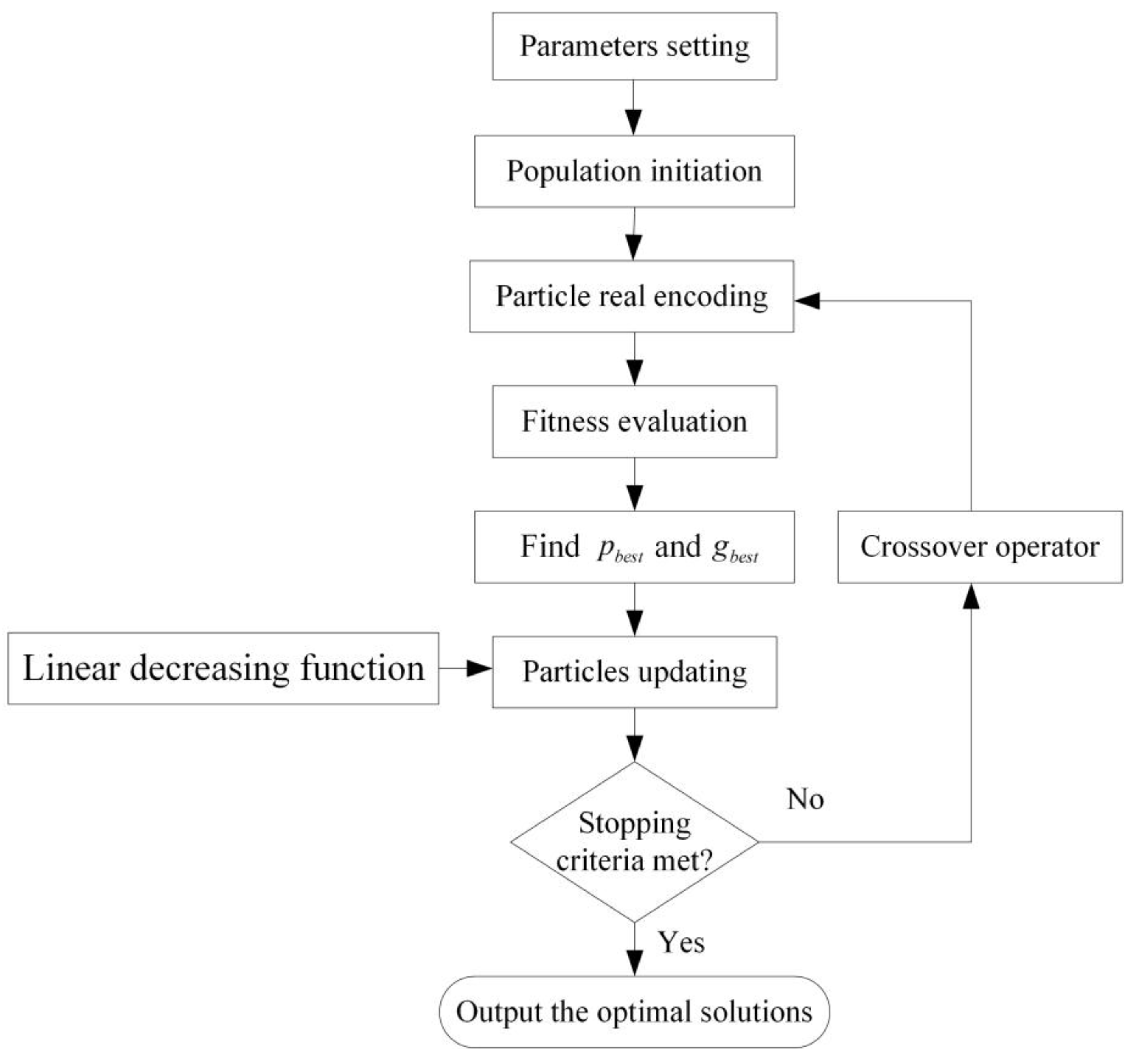
- (1)
- Parameters setting. Define the parameters: acceleration coefficients and , the maximum number of iterations , the initial value of inertia weight , the final value of inertia weight , a random number , the number of the particles , the maximum velocities of the particles .
- (2)
- Population initiation. Initialize particles as a population, generate the pth particle with random position , velocity , and personal best . Set iteration .
- (3)
- Particle encoding. According to the particle encoding rules, for , decode to a set of route .
- (4)
- Fitness evaluation. According to Equation (1), compute , and then evaluate through Equation (9).
- (5)
- and updating. Compute and . If , update . If , update .
- (6)
- Particles updating. Update the velocity and the position of each pth particle according to Equation (10).
- (7)
- Termination judgment. If the stopping criterion is met, go to step (9). Otherwise, and go to step (8). The stopping criterion is that or finding a better solution. A better solution means that the hierarchical cost objective value is better than that of the best solution found so far.
- (8)
- Crossover operator. Generate random number . According to Equations (13)–(16), generate a new set of population. Then return to step (3).
- (9)
- Outputting the optimal solution. Decode as the best set of vehicle route and output the optimal solution .
5. Experimental Results
5.1. Solomon Benchmark Problems
5.2. Evaluation of the Results
5.3. Analysis of the Results
5.3.1. The Total Traveled Distance
| No. | Problem | Best-Known Solution | Genetic | PSO | ACO | The Proposed Algorithm | |||||||||||||
|---|---|---|---|---|---|---|---|---|---|---|---|---|---|---|---|---|---|---|---|
| Best | Average | Best | Average | Best | Average | Best | Average | ||||||||||||
| TD | NV | TD | NV | TD | NV | TD | NV | TD | NV | TD | NV | TD | NV | TD | NV | TD | NV | ||
| 1 | C101 | 828.94 | 10 | 828.94 | 10 | 856.26 | 10.20 | 828.94 | 10 | 842.60 | 10.10 | 828.94 | 10 | 842.60 | 10.10 | 828.94 | 10 | 842.60 | 10.10 |
| 2 | C102 | 828.94 | 10 | 828.94 | 10 | 828.94 | 10.00 | 828.94 | 10 | 828.94 | 10.00 | 828.94 | 10 | 857.82 | 10.10 | 828.94 | 10 | 828.94 | 10.00 |
| 3 | C103 | 828.06 | 10 | 828.06 | 10 | 859.88 | 10.00 | 828.06 | 10 | 828.06 | 10.00 | 828.06 | 10 | 828.06 | 10.00 | 828.06 | 10 | 828.06 | 10.00 |
| 4 | C104 | 824.78 | 10 | 824.78 | 10 | 824.78 | 10.00 | 824.78 | 10 | 824.78 | 10.00 | 824.78 | 10 | 849.79 | 10.10 | 824.78 | 10 | 824.78 | 10.00 |
| 5 | C105 | 828.94 | 10 | 828.94 | 10 | 854.25 | 10.20 | 828.94 | 10 | 866.91 | 10.30 | 828.94 | 10 | 904.88 | 10.60 | 828.94 | 10 | 841.60 | 10.10 |
| 6 | C106 | 828.94 | 10 | 828.94 | 10 | 851.78 | 10.10 | 828.94 | 10 | 897.46 | 10.30 | 828.94 | 10 | 943.14 | 10.50 | 828.94 | 10 | 874.62 | 10.20 |
| 7 | C107 | 828.94 | 10 | 828.94 | 10 | 856.47 | 10.20 | 828.94 | 10 | 842.70 | 10.10 | 828.94 | 10 | 870.23 | 10.30 | 828.94 | 10 | 842.70 | 10.10 |
| 8 | C108 | 828.94 | 10 | 828.94 | 10 | 865.99 | 10.00 | 828.94 | 10 | 841.29 | 10.00 | 828.94 | 10 | 853.64 | 10.00 | 828.94 | 10 | 841.29 | 10.00 |
| 9 | C109 | 828.94 | 10 | 828.94 | 10 | 910.27 | 10.30 | 828.94 | 10 | 856.05 | 10.10 | 828.94 | 10 | 883.16 | 10.20 | 828.94 | 10 | 828.94 | 10.00 |
| 10 | C201 | 591.56 | 3 | 591.56 | 3 | 602.53 | 3.30 | 591.56 | 3 | 606.18 | 3.40 | 591.56 | 3 | 609.84 | 3.50 | 591.56 | 3 | 598.87 | 3.20 |
| 11 | C202 | 591.56 | 3 | 591.56 | 3 | 656.01 | 3.20 | 591.56 | 3 | 623.78 | 3.10 | 591.56 | 3 | 623.78 | 3.10 | 591.56 | 3 | 591.56 | 3.00 |
| 12 | C203 | 591.17 | 3 | 591.17 | 3 | 606.19 | 3.00 | 591.17 | 3 | 604.69 | 3.00 | 591.17 | 3 | 618.20 | 3.00 | 591.17 | 3 | 604.69 | 3.00 |
| 13 | C204 | 590.60 | 3 | 590.60 | 3 | 704.28 | 3.30 | 590.60 | 3 | 666.39 | 3.20 | 590.60 | 3 | 742.17 | 3.40 | 590.60 | 3 | 628.49 | 3.10 |
| 14 | C205 | 588.88 | 3 | 588.88 | 3 | 619.27 | 3.30 | 588.88 | 3 | 599.01 | 3.10 | 588.88 | 3 | 609.14 | 3.20 | 588.88 | 3 | 599.01 | 3.10 |
| 15 | C206 | 588.49 | 3 | 588.49 | 3 | 620.28 | 3.20 | 588.49 | 3 | 604.38 | 3.10 | 588.49 | 3 | 636.17 | 3.30 | 588.49 | 3 | 588.49 | 3.00 |
| 16 | C207 | 588.29 | 3 | 588.29 | 3 | 610.49 | 3.00 | 588.29 | 3 | 632.69 | 3.00 | 588.29 | 3 | 621.59 | 3.00 | 588.29 | 3 | 599.39 | 3.00 |
| 17 | C208 | 588.32 | 3 | 588.32 | 3 | 622.73 | 3.00 | 588.32 | 3 | 599.79 | 3.00 | 588.32 | 3 | 611.26 | 3.00 | 588.32 | 3 | 599.79 | 3.00 |
| 18 | R101 | 1483.57 | 16 | 1642.87 | 20 | 1645.83 | 19.50 | 1642.87 | 20 | 1645.33 | 19.50 | 1645.79 | 19 | 1647.29 | 19.00 | 1642.87 | 20 | 1645.83 | 19.50 |
| 19 | R102 | 1355.93 | 14 | 1482.74 | 18 | 1483.75 | 17.70 | 1472.62 | 18 | 1477.95 | 17.80 | 1480.73 | 18 | 1482.21 | 17.80 | 1472.62 | 18 | 1477.14 | 17.80 |
| 20 | R103 | 1133.35 | 12 | 1292.85 | 15 | 1248.88 | 14.40 | 1213.62 | 14 | 1239.30 | 14.40 | 1213.62 | 14 | 1247.22 | 14.30 | 1213.62 | 14 | 1239.01 | 13.80 |
| 21 | R104 | 968.28 | 10 | 982.01 | 10 | 995.05 | 9.60 | 1007.24 | 9 | 1007.30 | 9.00 | 982.01 | 10 | 1000.11 | 9.40 | 982.01 | 10 | 992.52 | 9.70 |
| 22 | R105 | 1262.53 | 12 | 1360.78 | 15 | 1366.87 | 14.80 | 1360.78 | 15 | 1374.14 | 14.70 | 1360.78 | 15 | 1369.99 | 15.30 | 1360.78 | 15 | 1366.42 | 15.00 |
| 23 | R106 | 1201.78 | 12 | 1249.40 | 13 | 1251.48 | 12.20 | 1241.52 | 13 | 1249.39 | 12.40 | 1251.98 | 12 | 1252.00 | 12.00 | 1241.52 | 13 | 1247.29 | 12.60 |
| 24 | R107 | 1051.92 | 11 | 1076.13 | 11 | 1094.18 | 10.70 | 1076.13 | 11 | 1094.19 | 10.50 | 1076.13 | 11 | 1096.08 | 10.70 | 1076.13 | 11 | 1088.49 | 10.70 |
| 25 | R108 | 948.57 | 10 | 963.99 | 9 | 965.42 | 9.90 | 963.99 | 9 | 965.10 | 9.70 | 948.57 | 10 | 960.92 | 9.60 | 948.57 | 10 | 955.82 | 9.60 |
| 26 | R109 | 1110.40 | 12 | 1151.84 | 13 | 1181.86 | 11.60 | 1151.84 | 13 | 1186.15 | 11.40 | 1151.84 | 13 | 1190.44 | 11.20 | 1151.84 | 13 | 1164.71 | 12.40 |
| 27 | R110 | 1080.36 | 11 | 1080.36 | 11 | 1112.79 | 10.30 | 1080.36 | 11 | 1105.14 | 10.50 | 1080.36 | 11 | 1107.72 | 10.50 | 1080.36 | 11 | 1098.14 | 10.70 |
| 28 | R111 | 987.80 | 10 | 1053.50 | 12 | 1086.43 | 10.80 | 1053.50 | 12 | 1083.13 | 11.60 | 1088.48 | 12 | 1095.07 | 10.40 | 1053.50 | 12 | 1069.14 | 11.60 |
| 29 | R112 | 953.63 | 10 | 982.14 | 9 | 995.33 | 10.80 | 953.63 | 10 | 965.03 | 10.00 | 953.63 | 10 | 987.40 | 10.60 | 960.68 | 10 | 968.58 | 9.90 |
| 30 | R201 | 1148.48 | 9 | 1148.48 | 9 | 1208.94 | 7.70 | 1179.79 | 9 | 1231.20 | 5.50 | 1148.48 | 9 | 1212.51 | 7.30 | 1148.48 | 9 | 1178.39 | 8.40 |
| 31 | R202 | 1049.74 | 7 | 1049.74 | 7 | 1086.62 | 5.70 | 1049.74 | 7 | 1100.68 | 5.00 | 1079.36 | 6 | 1142.69 | 4.10 | 1049.74 | 7 | 1081.57 | 5.70 |
| 32 | R203 | 900.08 | 5 | 900.08 | 5 | 930.23 | 4.60 | 932.76 | 7 | 939.72 | 3.80 | 939.54 | 3 | 941.70 | 3.00 | 900.08 | 5 | 922.71 | 4.60 |
| 33 | R204 | 772.33 | 4 | 807.38 | 4 | 828.06 | 2.40 | 772.33 | 4 | 817.42 | 2.80 | 772.33 | 4 | 823.17 | 2.80 | 772.33 | 4 | 801.47 | 3.40 |
| 34 | R205 | 959.74 | 4 | 970.89 | 6 | 982.66 | 4.50 | 970.89 | 6 | 980.30 | 4.80 | 970.89 | 6 | 989.71 | 3.60 | 970.89 | 6 | 977.95 | 5.10 |
| 35 | R206 | 898.91 | 5 | 898.91 | 5 | 906.06 | 3.40 | 906.14 | 3 | 910.24 | 3.00 | 906.14 | 3 | 912.29 | 3.00 | 898.91 | 5 | 903.89 | 4.00 |
| 36 | R207 | 814.78 | 3 | 814.78 | 3 | 844.73 | 3.40 | 814.78 | 3 | 868.25 | 2.60 | 814.78 | 3 | 876.51 | 2.60 | 814.78 | 3 | 836.67 | 3.00 |
| 37 | R208 | 715.37 | 3 | 725.75 | 2 | 726.61 | 2.00 | 725.42 | 4 | 725.77 | 3.20 | 725.75 | 2 | 726.71 | 2.00 | 723.61 | 3 | 725.50 | 2.50 |
| 38 | R209 | 879.53 | 6 | 879.53 | 6 | 892.08 | 5.40 | 879.53 | 6 | 891.00 | 5.40 | 879.53 | 6 | 903.21 | 4.20 | 879.53 | 6 | 891.82 | 5.10 |
| 39 | R210 | 932.89 | 7 | 954.12 | 3 | 955.06 | 6.60 | 954.12 | 3 | 954.64 | 5.00 | 939.34 | 3 | 952.94 | 4.78 | 932.89 | 7 | 937.89 | 6.20 |
| 40 | R211 | 761.10 | 4 | 885.71 | 2 | 892.31 | 2.30 | 885.71 | 2 | 889.53 | 4.40 | 888.73 | 5 | 867.07 | 2.90 | 808.56 | 4 | 824.99 | 3.90 |
| 41 | RC101 | 1481.27 | 13 | 1660.10 | 16 | 1689.57 | 14.40 | 1623.58 | 15 | 1658.18 | 15.10 | 1639.97 | 16 | 1687.56 | 14.40 | 1623.58 | 15 | 1645.18 | 15.10 |
| 42 | RC102 | 1395.25 | 13 | 1466.84 | 14 | 1493.53 | 13.50 | 1482.91 | 14 | 1497.28 | 13.60 | 1477.54 | 13 | 1539.85 | 12.30 | 1466.84 | 14 | 1487.10 | 13.50 |
| 43 | RC103 | 1221.53 | 10 | 1261.67 | 11 | 1263.56 | 11.00 | 1262.02 | 11 | 1262.29 | 11.00 | 1262.02 | 11 | 1264.17 | 11.00 | 1261.67 | 11 | 1262.04 | 11.00 |
| 44 | RC104 | 1135.48 | 10 | 1135.48 | 10 | 1135.50 | 10.00 | 1135.48 | 10 | 1135.50 | 10.00 | 1135.48 | 10 | 1135.51 | 10.00 | 1135.48 | 10 | 1135.49 | 10.00 |
| 45 | RC105 | 1354.20 | 12 | 1518.60 | 16 | 1601.17 | 15.40 | 1518.60 | 16 | 1593.35 | 14.80 | 1629.44 | 13 | 1633.29 | 13.00 | 1618.55 | 16 | 1621.16 | 15.40 |
| 46 | RC106 | 1226.62 | 11 | 1377.35 | 13 | 1396.59 | 11.80 | 1384.92 | 12 | 1417.25 | 11.20 | 1377.35 | 13 | 1416.49 | 11.30 | 1377.35 | 13 | 1392.80 | 12.30 |
| 47 | RC107 | 1150.99 | 10 | 1230.48 | 11 | 1254.98 | 12.60 | 1212.83 | 12 | 1240.50 | 12.30 | 1230.48 | 11 | 1258.04 | 12.80 | 1212.83 | 12 | 1226.01 | 12.00 |
| 48 | RC108 | 1076.81 | 10 | 1117.53 | 11 | 1135.32 | 10.30 | 1117.53 | 11 | 1127.41 | 10.90 | 1117.53 | 11 | 1128.55 | 10.80 | 1117.53 | 11 | 1126.40 | 10.70 |
| 49 | RC201 | 1134.91 | 6 | 1406.91 | 4 | 1391.43 | 7.20 | 1406.91 | 4 | 1406.91 | 4.00 | 1286.83 | 9 | 1397.23 | 6.00 | 1387.55 | 8 | 1391.43 | 7.20 |
| 50 | RC202 | 1113.53 | 8 | 1365.57 | 4 | 1250.18 | 3.60 | 1113.53 | 8 | 1162.75 | 7.60 | 1113.53 | 8 | 1204.86 | 6.30 | 1148.84 | 9 | 1173.34 | 7.90 |
| 51 | RC203 | 945.96 | 5 | 945.96 | 5 | 1034.30 | 3.40 | 945.96 | 5 | 1032.14 | 3.40 | 1049.62 | 3 | 1052.87 | 3.00 | 945.96 | 5 | 990.67 | 4.20 |
| 52 | RC204 | 796.11 | 4 | 798.41 | 3 | 798.69 | 3.20 | 798.41 | 3 | 799.18 | 3.60 | 798.46 | 3 | 799.43 | 3.80 | 798.41 | 3 | 798.67 | 3.20 |
| 53 | RC205 | 1168.22 | 8 | 1270.69 | 7 | 1276.08 | 6.40 | 1168.22 | 8 | 1282.01 | 4.70 | 1168.22 | 8 | 1263.14 | 6.80 | 1161.81 | 7 | 1187.56 | 6.90 |
| 54 | RC206 | 1059.89 | 7 | 1059.89 | 7 | 1105.75 | 5.80 | 1084.30 | 8 | 1139.24 | 4.00 | 1059.89 | 7 | 1135.44 | 4.00 | 1059.89 | 7 | 1092.22 | 6.00 |
| 55 | RC207 | 976.40 | 7 | 999.26 | 6 | 1060.37 | 3.60 | 976.40 | 7 | 1011.75 | 5.70 | 1053.58 | 6 | 1064.28 | 3.90 | 976.40 | 7 | 995.65 | 6.40 |
| 56 | RC208 | 785.93 | 4 | 816.10 | 5 | 824.93 | 3.60 | 816.10 | 5 | 822.41 | 4.00 | 806.87 | 5 | 819.64 | 4.00 | 795.39 | 5 | 807.27 | 4.78 |
5.3.2. The Average Total Traveled Distance
| Problem | Best-Known Solution | Genetic | PSO | ACO | The Proposed Algorithm | |||||
|---|---|---|---|---|---|---|---|---|---|---|
| Best | Average | Best | Average | Best | Average | Best | Average | |||
| C1-type | NV | 10.00 | 10.00 | 10.11 | 10.00 | 10.10 | 10.00 | 10.21 | 10.00 | 10.06 |
| TD | 828.38 | 828.38 | 856.51 | 828.38 | 847.64 | 828.38 | 870.37 | 828.38 | 839.28 | |
| C2-type | NV | 3.00 | 3.00 | 3.16 | 3.00 | 3.11 | 3.00 | 3.19 | 3.00 | 3.05 |
| TD | 589.86 | 589.86 | 630.22 | 589.86 | 617.11 | 589.86 | 634.02 | 589.86 | 601.29 | |
| R1-type | NV | 11.67 | 13.00 | 12.69 | 12.92 | 12.63 | 12.92 | 12.57 | 13.08 | 12.78 |
| TD | 1128.18 | 1193.22 | 1202.32 | 1184.84 | 1199.35 | 1186.16 | 1203.04 | 1182.04 | 1192.76 | |
| R2-type | NV | 5.18 | 4.73 | 4.36 | 4.91 | 4.14 | 4.55 | 3.66 | 5.36 | 4.72 |
| TD | 893.90 | 912.31 | 932.12 | 915.56 | 937.16 | 914.99 | 940.77 | 899.98 | 916.62 | |
| RC1-type | NV | 11.13 | 12.75 | 12.38 | 12.63 | 12.36 | 12.25 | 11.95 | 12.75 | 12.50 |
| TD | 1255.27 | 1346.01 | 1371.28 | 1342.23 | 1366.47 | 1358.73 | 1382.93 | 1351.73 | 1362.02 | |
| RC2-type | NV | 6.13 | 5.13 | 4.60 | 6.00 | 4.63 | 6.13 | 4.73 | 6.38 | 5.82 |
| TD | 997.62 | 1082.85 | 1092.72 | 1038.73 | 1082.05 | 1042.13 | 1092.11 | 1034.28 | 1054.60 | |
| All | NV | 449 | 465 | 452.40 | 472 | 448.70 | 466 | 441.88 | 483 | 466.68 |
| TD | 53,568.46 | 55,959.11 | 57,143.53 | 55,511.30 | 56,854.75 | 55,679.89 | 57,490.75 | 55,346.67 | 56,092.75 | |
5.3.3. The Average Central Processing Unit (CPU) Runtime
| Problem | Genetic | PSO | ACO | The Proposed Algorithm |
|---|---|---|---|---|
| C1e | 98 | 85 | 111 | 62 |
| C2 | 312 | 231 | 338 | 135 |
| R1 | 112 | 81 | 124 | 60 |
| R2 | 309 | 273 | 553 | 182 |
| RC1 | 79 | 80 | 82 | 58 |
| RC2 | 297 | 257 | 333 | 149 |
5.3.4. The Quality of the Solutions
| Problem | Genetic | PSO | ACO | The Proposed Algorithm |
|---|---|---|---|---|
| C1-type | 3.39% | 2.32% | 5.07% | 1.32% |
| C2-type | 6.84% | 4.62% | 7.48% | 1.94% |
| R1-type | 6.28% | 5.98% | 6.33% | 5.36% |
| R2-type | 4.44% | 4.93% | 5.29% | 2.62% |
| RC1-type | 8.89% | 8.53% | 9.75% | 8.17% |
| RC2-type | 8.96% | 7.92% | 8.95% | 5.30% |
| All | 6.29% | 5.63% | 6.95% | 4.07% |
6. Conclusions
- (1)
- The real encoding method avoids the complex encoding and decoding computation burden.
- (2)
- A linear decreasing function of the number of iterations in PSO have a flexible and well-balanced mechanism to enhance and adapt to the global and local exploration abilities, which can help find the optimal solution with the least number of iterations.
- (3)
- The crossover operator of the genetic algorithm is introduced to generate a new population guaranteeing that the offspring inherits good qualities from this parent. The crossover operator avoids premature convergence and local minimum value and increases the diversity of particles.
Acknowledgements
Author Contributions
Conflicts of Interest
References
- Dantzig, G.; Ramser, J. The truck dispatching problem. Manag. Sci. 1959, 6, 80–91. [Google Scholar] [CrossRef]
- Hu, W.; Liang, H.; Peng, C.; Du, B.; Hu, Q. A hybrid chaos-particle swarm optimization algorithm for the vehicle routing problem with time window. Entropy 2013, 15, 1247–1270. [Google Scholar] [CrossRef]
- Bräysy, O. A reactive variable neighborhood search for the vehicle-routing problem with time windows. INFORMS J. Comput. 2003, 15, 347–368. [Google Scholar] [CrossRef]
- Belenguer, J.-M.; Benavent, E.; Prins, C.; Prodhon, C.; Calvo, R.W. A branch-and-cut method for the capacitated location-routing problem. Comput. Oper. Res. 2011, 38, 931–941. [Google Scholar] [CrossRef]
- Jepsen, M.; Spoorendonk, S.; Ropke, S. A branch-and-cut algorithm for the symmetric two-echelon capacitated vehicle routing problem. Transp. Sci. 2013, 47, 23–37. [Google Scholar] [CrossRef]
- Niebles, J.; Wang, H.; Fei-Fei, L. Unsupervised learning of human action categories using spatial-temporal words. Int. J. Comput. Vis. 2008, 79, 299–318. [Google Scholar] [CrossRef]
- Vidal, T.; Crainic, T.G.; Gendreau, M.; Prins, C. Heuristics for multi-attribute vehicle routing problems: A survey and synthesis. Eur. J. Oper. Res. 2013, 231, 1–21. [Google Scholar] [CrossRef]
- Berbeglia, G.; Cordeau, J.-F.; Laporte, G. A hybrid tabu search and constraint programming algorithm for the dynamic dial-a-ride problem. INFORMS J. Comput. 2012, 24, 343–355. [Google Scholar] [CrossRef]
- Pillac, V.; Gendreau, M.; Guéret, C.; Medaglia, A.L. A review of dynamic vehicle routing problems. Eur. J. Oper. Res. 2013, 225, 1–11. [Google Scholar] [CrossRef] [Green Version]
- Andres Figliozzi, M. The time dependent vehicle routing problem with time windows: Benchmark problems, an efficient solution algorithm, and solution characteristics. Transp. Res. Part E Logist. Transp. Rev. 2012, 48, 616–636. [Google Scholar] [CrossRef]
- Çetinkaya, C.; Karaoglan, I.; Gökçen, H. Two-stage vehicle routing problem with arc time windows: A mixed integer programming formulation and a heuristic approach. Eur. J. Oper. Res. 2013, 230, 539–550. [Google Scholar] [CrossRef]
- Yu, B.; Yang, Z.; Yao, B. A hybrid algorithm for vehicle routing problem with time windows. Expert Syst. Appl. 2011, 38, 435–441. [Google Scholar] [CrossRef]
- Anbuudayasankar, S.; Ganesh, K.; Koh, S.L.; Ducq, Y. Modified savings heuristics and genetic algorithm for bi-objective vehicle routing problem with forced backhauls. Expert Syst. Appl. 2012, 39, 2296–2305. [Google Scholar] [CrossRef]
- Repoussis, P.P.; Tarantilis, C.D.; Ioannou, G. Arc-guided evolutionary algorithm for the vehicle routing problem with time windows. IEEE Trans. Evol. Comput. 2009, 13, 624–647. [Google Scholar] [CrossRef]
- Garcia-Najera, A.; Bullinaria, J.A. An improved multi-objective evolutionary algorithm for the vehicle routing problem with time windows. Comput. Oper. Res. 2011, 38, 287–300. [Google Scholar] [CrossRef]
- Prescott-Gagnon, E.; Desaulniers, G.; Rousseau, L.M. A branch-and-price-based large neighborhood search algorithm for the vehicle routing problem with time windows. Networks 2009, 54, 190–204. [Google Scholar] [CrossRef]
- Azi, N.; Gendreau, M.; Potvin, J.Y. An exact algorithm for a vehicle routing problem with time windows and multiple use of vehicles. Eur. J. Oper. Res. 2010, 202, 756–763. [Google Scholar] [CrossRef]
- Cordeau, J.F.; Maischberger, M. A parallel iterated tabu search heuristic for vehicle routing problems. Comput. Oper. Res. 2012, 39, 2033–2050. [Google Scholar] [CrossRef]
- Brandão, J. A tabu search algorithm for the heterogeneous fixed fleet vehicle routing problem. Comput. Oper. Res. 2011, 38, 140–151. [Google Scholar] [CrossRef]
- Escobar, J.W.; Linfati, R.; Toth, P.; Baldoquin, M.G. A hybrid granular tabu search algorithm for the multi-depot vehicle routing problem. J. Heuristics 2014, 20, 483–509. [Google Scholar] [CrossRef]
- Archetti, C.; Bouchard, M.; Desaulniers, G. Enhanced branch and price and cut for vehicle routing with split deliveries and time windows. Transp. Sci. 2011, 45, 285–298. [Google Scholar] [CrossRef]
- Hashimoto, H.; Yagiura, M.; Ibaraki, T. An iterated local search algorithm for the time-dependent vehicle routing problem with time windows. Discret. Opt. 2008, 5, 434–456. [Google Scholar] [CrossRef]
- Michallet, J.; Prins, C.; Amodeo, L.; Yalaoui, F.; Vitry, G. Multi-start iterated local search for the periodic vehicle routing problem with time windows and time spread constraints on services. Comput. Oper. Res. 2014, 41, 196–207. [Google Scholar] [CrossRef]
- Li, X.; Tian, P.; Leung, S.C.H. Vehicle routing problems with time windows and stochastic travel and service times: Models and algorithm. Int. J. Prod. Econ. 2010, 125, 137–145. [Google Scholar] [CrossRef]
- Yu, B.; Yang, Z.Z. An ant colony optimization model: The period vehicle routing problem with time windows. Transp. Res. Part E Logist. Transp. Rev. 2011, 47, 166–181. [Google Scholar] [CrossRef]
- Dhahri, A.; Zidi, K.; Ghedira, K. A Variable Neighborhood Search for the Vehicle Routing Problem with Time Windows and Preventive Maintenance Activities. Electron. Notes Discret. Math. 2015, 47, 229–236. [Google Scholar] [CrossRef]
- Khouadjia, M.R.; Sarasola, B.; Alba, E.; Jourdan, L.; Talbi, E.-G. A comparative study between dynamic adapted PSO and VNS for the vehicle routing problem with dynamic requests. Appl. Soft Comput. 2012, 12, 1426–1439. [Google Scholar] [CrossRef]
- Brandão de Oliveira, H.C.; Vasconcelos, G.C. A hybrid search method for the vehicle routing problem with time windows. Ann. Oper. Res. 2010, 180, 125–144. [Google Scholar] [CrossRef]
- Balseiro, S.; Loiseau, I.; Ramonet, J. An Ant Colony algorithm hybridized with insertion heuristics for the Time Dependent Vehicle Routing Problem with Time Windows. Comput. Oper. Res. 2011, 38, 954–966. [Google Scholar] [CrossRef]
- Szeto, W.; Wu, Y.; Ho, S.C. An artificial bee colony algorithm for the capacitated vehicle routing problem. Eur. J. Oper. Res. 2011, 215, 126–135. [Google Scholar] [CrossRef] [Green Version]
- Mahdavi, V.; Sadeghi, S.A.; Fathi, S. A mathematical Model and Solving Method for Multi-Depot and Multi-level Vehicle Routing Problem with Fuzzy Time Windows. Adv. Intel. Transp. Syst. 2012, 1, 19–24. [Google Scholar]
- El-Sherbeny, N.A. Vehicle routing with time windows: An overview of exact, heuristic and metaheuristic methods. J. King Saud Univ. Sci. 2010, 22, 123–131. [Google Scholar] [CrossRef]
- Bhagade, A.S.; Puranik, P.V. Artificial bee colony (ABC) algorithm for vehicle routing optimization problem. Int. J. Soft Comput. Eng. 2012, 2, 329–333. [Google Scholar]
- Ai, T.; Kachitvichyanukul, V. A particle swarm optimization for the vehicle routing problem with simultaneous pickup and delivery. Comput. Oper. Res. 2009, 36, 1693–1702. [Google Scholar] [CrossRef]
- Kok, A.L.; Meyer, C.M.; Kopfer, H.; Schutten, J.M.J. A dynamic programming heuristic for the vehicle routing problem with time windows and European Community social legislation. Transp. Sci. 2010, 44, 442–454. [Google Scholar] [CrossRef]
- Erdoğan, S.; Miller-Hooks, E. A green vehicle routing problem. Transp. Res. Part E Logist. Transp. Rev. 2012, 48, 100–114. [Google Scholar] [CrossRef]
- Küçükoğlu, İ.; Öztürk, N. An advanced hybrid meta-heuristic algorithm for the vehicle routing problem with backhauls and time windows. Comput. Ind. Eng. 2015, 86, 60–68. [Google Scholar] [CrossRef]
- Marinakis, Y.; Marinaki, M. A hybrid genetic–Particle Swarm Optimization Algorithm for the vehicle routing problem. Expert Syst. Appl. 2010, 37, 1446–1455. [Google Scholar] [CrossRef]
- Nagata, Y.; Bräysy, O.; Dullaert, W. A penalty-based edge assembly memetic algorithm for the vehicle routing problem with time windows. Comput. Oper. Res. 2010, 37, 724–737. [Google Scholar] [CrossRef]
- Dey, S.; Bhattacharyya, S.; Maulik, U. Quantum inspired genetic algorithm and particle swarm optimization using chaotic map model based interference for gray level image thresholding. Swarm Evol. Comput. 2014, 15, 38–57. [Google Scholar] [CrossRef]
- Valdez, F.; Melin, P.; Castillo, O. Modular neural networks architecture optimization with a new nature inspired method using a fuzzy combination of particle swarm optimization and genetic algorithms. Inf. Sci. 2014, 270, 143–153. [Google Scholar] [CrossRef]
- Ru, N.; Yue, J. A GA and particle swarm optimization based hybrid algorithm. In Proceedings of the IEEE Congress on Evolutionary Computation, Hong Kong, China, 1–6 June 2008; pp. 1047–1050.
- Hao, Z.-F.; Wang, Z.-G.; Huang, H. A particle swarm optimization algorithm with crossover operator. In Proceedings of the 2007 IEEE International Conference on Machine Learning and Cybernetics, Hong Kong, China, 19–22 August 2007; pp. 1036–1040.
- Masrom, S.; Abidin, S.Z.; Omar, N.; Nasir, K.; Abd Rahman, A. Dynamic parameterization of the particle swarm optimization and genetic algorithm hybrids for vehicle routing problem with time window. Int. J. Hybrid Int. Syst. 2015, 12, 13–25. [Google Scholar]
- Kuo, R.; Zulvia, F.E.; Suryadi, K. Hybrid particle swarm optimization with genetic algorithm for solving capacitated vehicle routing problem with fuzzy demand—A case study on garbage collection system. Appl. Math. Comput. 2012, 219, 2574–2588. [Google Scholar] [CrossRef]
- Dhahri, A.; Zidi, K.; Ghedira, K. Variable Neighborhood Search based Set Covering ILP Model for the Vehicle Routing Problem with Time Windows. Proc. Comput. Sci. 2014, 29, 844–854. [Google Scholar] [CrossRef]
- Sha, D.; Hsu, C. A new particle swarm optimization for the open shop scheduling problem. Comput. Oper. Res. 2008, 35, 3243–3261. [Google Scholar] [CrossRef]
- Lian, Z.; Gu, X.; Jiao, B. A novel particle swarm optimization algorithm for permutation flow-shop scheduling to minimize makespan. Chaos Solitons Fract. 2008, 35, 851–861. [Google Scholar] [CrossRef]
- Jarboui, B.; Damak, N.; Siarry, P.; Rebai, A. A combinatorial particle swarm optimization for solving multi-mode resource-constrained project scheduling problems. Appl. Math. Comput. 2008, 195, 299–308. [Google Scholar] [CrossRef]
- Shi, X.; Liang, Y.; Lee, H.; Lu, C.; Wang, Q. Particle swarm optimization-based algorithms for TSP and generalized TSP. Inf. Process. Lett. 2007, 103, 169–176. [Google Scholar] [CrossRef]
- Jarboui, B.; Cheikh, M.; Siarry, P.; Rebai, A. Combinatorial particle swarm optimization (CPSO) for partitional clustering problem. Appl. Math. Comput. 2007, 192, 337–345. [Google Scholar] [CrossRef]
- Pan, Q.; Fatih Tasgetiren, M.; Liang, Y. A discrete particle swarm optimization algorithm for the no-wait flowshop scheduling problem. Comput. Oper. Res. 2008, 35, 2807–2839. [Google Scholar] [CrossRef]
- Yin, P.-Y.; Yu, S.-S.; Wang, P.-P.; Wang, Y.-T. A hybrid particle swarm optimization algorithm for optimal task assignment in distributed systems. Comput. Stand. Int. 2006, 28, 441–450. [Google Scholar] [CrossRef]
- Bohre, A.K.; Agnihotri, G.; Dubey, M.; Singh, J. A Novel Method to Find Optimal Solution Based on Modified Butterfly Particle Swarm Optimization. Int. J. Soft Comput. Math. Control 2014, 3, 1–14. [Google Scholar] [CrossRef]
- Ping, H.J.; Lian, L.Y.; Xing, H.; Hua, W.J. A Novel Hybrid Algorithm with Marriage of Particle Swarm Optimization and Homotopy Optimization for Tunnel Parameter Inversion. Appl. Mech. Mater. 2012, 229–231, 2033–2037. [Google Scholar]
- Shi, Y.; Eberhart, R. A modified particle swarm optimizer. In Proceedings of the IEEE International Conference on Evolutionary Computation, Anchorage, AK, USA, 4–9 May 1998; pp. 69–73.
- Jiao, B.; Lian, Z.; Gu, X. A dynamic inertia weight particle swarm optimization algorithm. Chaos Solitons Fract. 2008, 37, 698–705. [Google Scholar] [CrossRef]
- Liu, X.; Wang, Q.; Liu, H.; Li, L. Particle swarm optimization with dynamic inertia weight and mutation. In Porceedings of the 3rd IEEE International Conference on Genetic and Evolutionary Computing, Guilin, China, 14–17 October 2009; pp. 620–623.
- Tao, Z.; Cai, J. A new chaotic PSO with dynamic inertia weight for economic dispatch problem. In Proceedings of the IEEE International Conference on Sustainable Power Generation and Supply, Nanjing, China, 6–7 April 2009; pp. 1–6.
- Tripathi, P.K.; Bandyopadhyay, S.; Pal, S.K. Multi-objective particle swarm optimization with time variant inertia and acceleration coefficients. Inf. Sci. 2007, 177, 5033–5049. [Google Scholar] [CrossRef]
- Nickabadi, A.; Ebadzadeh, M.M.; Safabakhsh, R. A novel particle swarm optimization algorithm with adaptive inertia weight. Appl. Soft Comput. 2011, 11, 3658–3670. [Google Scholar] [CrossRef]
- Shen, X.; Chi, Z.; Yang, J.; Chen, C. Particle swarm optimization with dynamic adaptive inertia weight. In Proceedings of the IEEE International Conference on Challenges in Environmental Science and Computer Engineering, Wuhan, China, 6–9 March 2010; pp. 287–290.
- Zhang, L.; Tang, Y.; Hua, C.; Guan, X. A new particle swarm optimization algorithm with adaptive inertia weight based on Bayesian techniques. Appl. Soft Comput. 2015, 28, 138–149. [Google Scholar] [CrossRef]
- VRPTW Benchmark Problems. Available online: http://web.cba.neu.edu/~msolomon/problems.htm (accessed on 26 August 2015).
- Ai, T.J.; Kachitvichyanukul, V. A particle swarm optimisation for vehicle routing problem with time windows. Int. J. Oper. Res. 2009, 6, 519–537. [Google Scholar] [CrossRef]
- Baños, R.; Ortega, J.; Gil, C.; Márquez, A.L.; de Toro, F. A hybrid meta-heuristic for multi-objective vehicle routing problems with time windows. Comput. Ind. Eng. 2013, 65, 286–296. [Google Scholar] [CrossRef]
- Barbucha, D. A cooperative population learning algorithm for vehicle routing problem with time windows. Neurocomputing 2014, 146, 210–229. [Google Scholar] [CrossRef]
- Ghannadpour, S.F.; Noori, S.; Tavakkoli-Moghaddam, R.; Ghoseiri, K. A multi-objective dynamic vehicle routing problem with fuzzy time windows: Model, solution and application. Appl. Soft Comput. 2014, 14, 504–527. [Google Scholar] [CrossRef]
- Taş, D.; Jabali, O.; van Woensel, T. A vehicle routing problem with flexible time windows. Comput. Oper. Res. 2014, 52, 39–54. [Google Scholar] [CrossRef]
- Barb, A.S.; Shyu, C.R. A study of factors that influence the accuracy of content-based geospatial ranking systems. Int. J. Image Data Fusion 2012, 3, 257–268. [Google Scholar] [CrossRef]
- Alvarenga, G.B.; Mateus, G.R.; de Tomi, G. A genetic and set partitioning two-phase approach for the vehicle routing problem with time windows. Comput. Oper. Res. 2007, 34, 1561–1584. [Google Scholar] [CrossRef]
© 2015 by the authors; licensee MDPI, Basel, Switzerland. This article is an open access article distributed under the terms and conditions of the Creative Commons Attribution license (http://creativecommons.org/licenses/by/4.0/).
Share and Cite
Xu, S.-H.; Liu, J.-P.; Zhang, F.-H.; Wang, L.; Sun, L.-J. A Combination of Genetic Algorithm and Particle Swarm Optimization for Vehicle Routing Problem with Time Windows. Sensors 2015, 15, 21033-21053. https://doi.org/10.3390/s150921033
Xu S-H, Liu J-P, Zhang F-H, Wang L, Sun L-J. A Combination of Genetic Algorithm and Particle Swarm Optimization for Vehicle Routing Problem with Time Windows. Sensors. 2015; 15(9):21033-21053. https://doi.org/10.3390/s150921033
Chicago/Turabian StyleXu, Sheng-Hua, Ji-Ping Liu, Fu-Hao Zhang, Liang Wang, and Li-Jian Sun. 2015. "A Combination of Genetic Algorithm and Particle Swarm Optimization for Vehicle Routing Problem with Time Windows" Sensors 15, no. 9: 21033-21053. https://doi.org/10.3390/s150921033