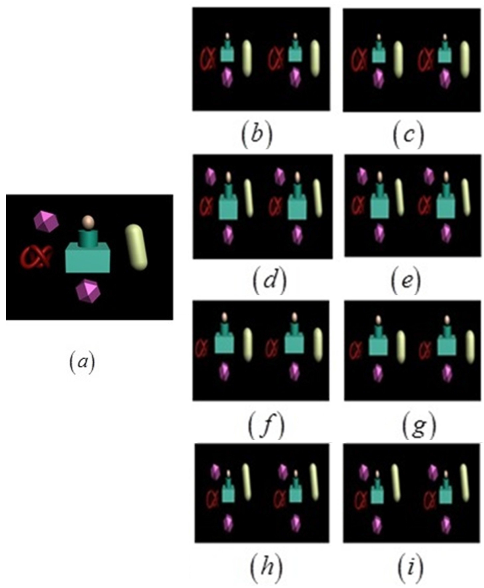
Figure 2.
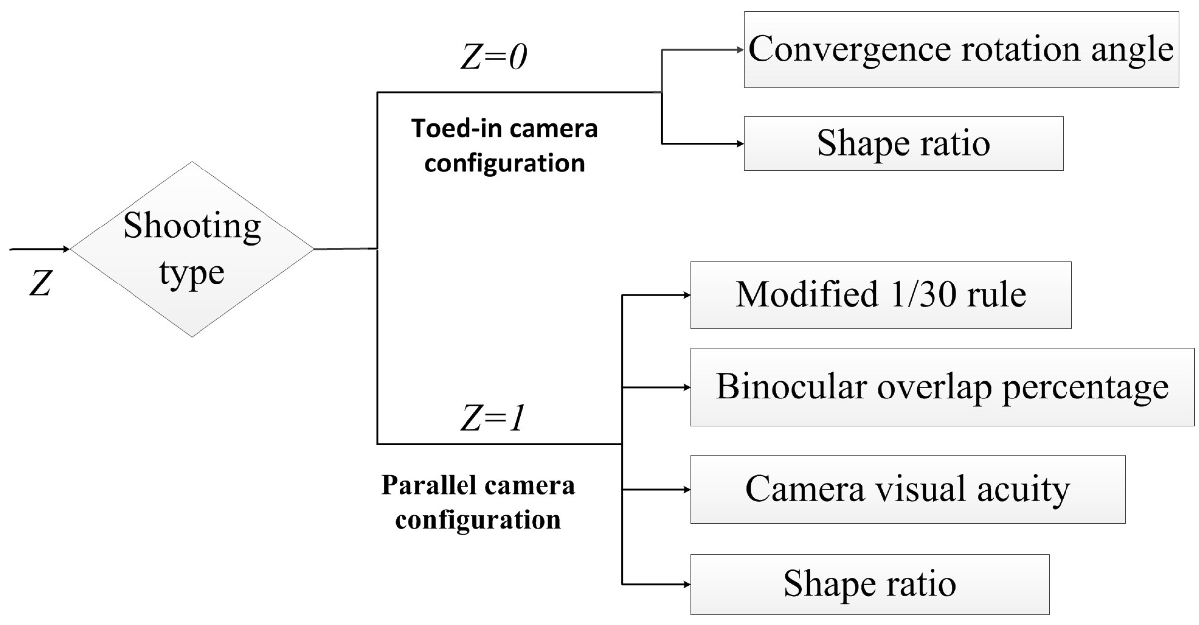
Objective stereo cameras’ shooting quality evaluation criteria for long distances.
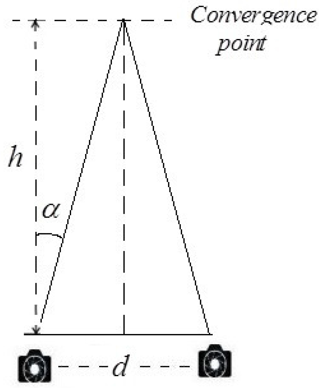
4.1. Evaluation Criterion for the Toed-In Camera Configuration
For the toed-in camera configuration, the optical axes are converging on a single point. The objects in the foreground have a significant effect on the stereo quality of the images. Convergence rotation angle
α [
25] and shape ratio
μ [
10] are important factors that have to be taken into consideration for the toed-in camera configuration over long-distance shooting.
Convergence rotation angle: Heinzle
et al. [
25] presented that the value of convergence rotation angle
α (Equation (1)) has an effect on the position of convergence point, as shown in
Figure 3.
Figure 3.
Computation of screen space disparities.
Figure 3.
Computation of screen space disparities.
Previous studies indicated that α had an effect on the screen disparity of a given point, while it referred to the distance between the two corresponding points in stereoscopic images recorded by the left and right cameras. The disparity was often the most important parameter for stereo depth perception and related to the most comfort-zone constraints. However, it was an empirical method and could only generate a rough estimation for camera parameters. Hence, this part of the whole aims to establish a corresponding five-level evaluation criterion of the convergence rotation angle for stereo cameras through subjective and objective experiments.
As a matter of convenience, this paper considered
α as the evaluation index. Firstly, when
f = 50 mm and
h was a fixed value,
d changed constantly. Then, we change the value of
h, and we captured the corresponding stereoscopic image pairs once again. Besides, we changed the camera focal length
f and carried out similar experiments as described above. The subjective results are shown in
Figure 4, and it was indicated that
f, as well as the
α value had a great effect on the subjective results.
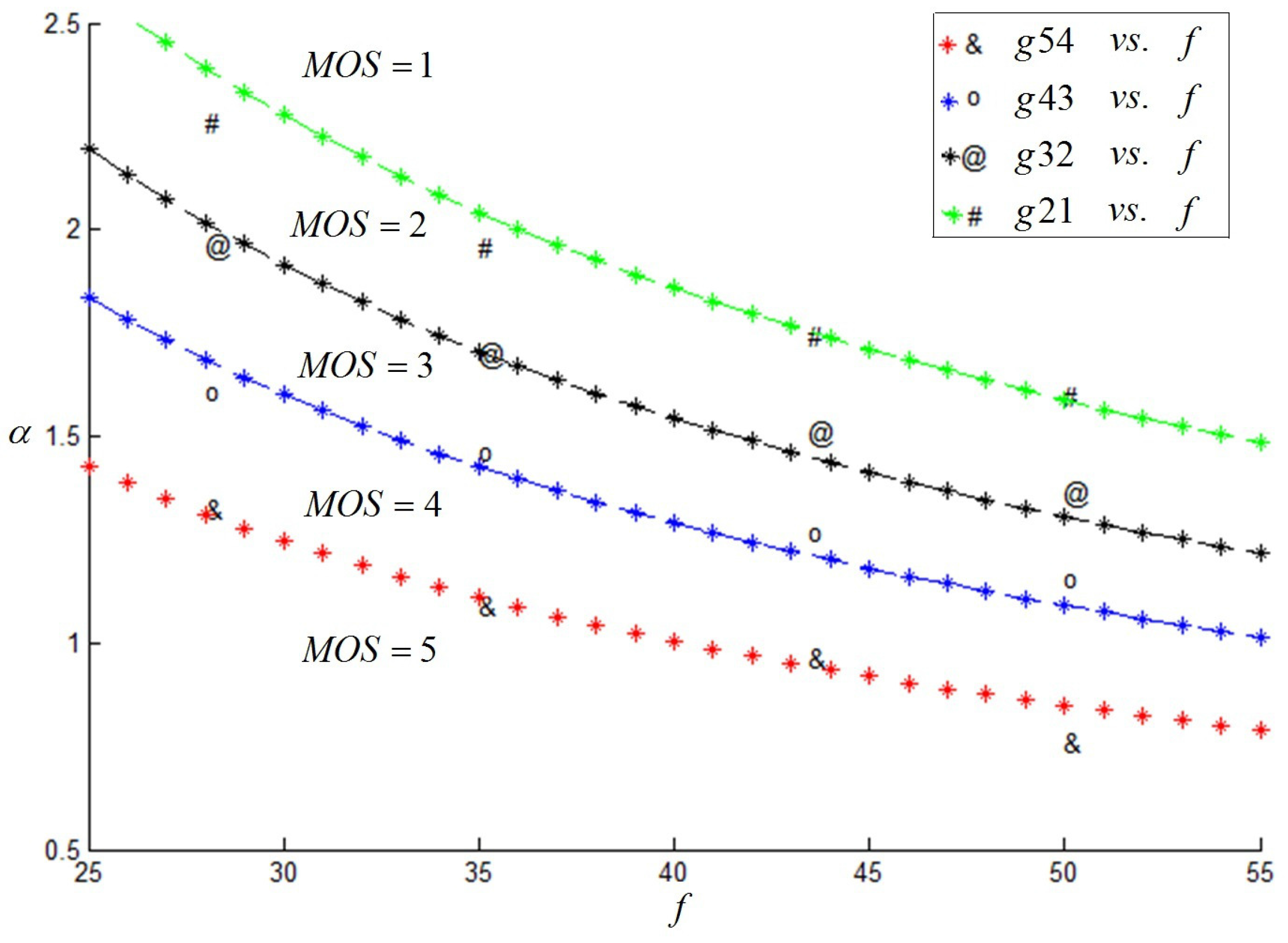
Figure 4.
Variation trend of α(°) with f (mm).
Figure 4.
Variation trend of α(°) with f (mm).
In order to enrich the experiments, several of the camera focal lengths were involved in our experiments. Through a number of experiments, we proposed an ultimate assessment index
g, calculated from Equation (2). The mapping between
g and the MOS value,
, was studied based on the subjective experimental results and is listed in
Table 3. It indicated that when the
g value was at most 20.56, a good stereoscopic effect could be obtained.
Table 3.
Mapping between g and the mean opinion score (MOS) value.
Table 3.
Mapping between g and the mean opinion score (MOS) value.
| Index: g |
|---|
| 5 | g≤16.00 |
| 4 | 16.00<g≤20.56 |
| 3 | 20.56<g≤24.61 |
| 2 | 24.61<g≤25.09 |
| 1 | g>25.09 |
Shape ratio: Frederik
et al. [
10] proposed that the shape ratio
μ was defined as the depth magnification to the width magnification. Equation (3) can be taken to ensure an undistorted depth reproduction near the screen surface:
Where is the viewing distance, is the viewer’s inter-ocular distance, h is the shooting distance and d is the inter-camera distance. Note that, if an average and the point of convergence are given, the grade of stereoscopic distortion can only be controlled by choosing the right ratio between d and .
The geometrical interpretation of Equation (3) depended on whether the points at infinity were actually presented in the captured scene. The value of μ had a significant effect on the quality of the stereoscopic image pairs. The smaller the value, the higher the stereo quality. Hence, when shooting long distance, h was far outstrips and d was bigger than . This part of the whole aims to establish a corresponding five-level evaluation criterion of the shape ratio for the stereo camera through experiments.
Based on the experiments, a series of stereoscopic image pairs was captured with different shape ratios. We selected a bigger viewing distance as 3.9 m; refer to [
36] for HDTV. The range of
μ is from 0.095 to 1.532. Through subjective experiments, we determined the mapping between
μ and the MOS value,
, of stereoscopic image pairs, shown in
Table 4, which indicated that when the
μ value was no more than 0.304, a good stereoscopic effect could be obtained.
Table 4.
Mapping between μ and the MOS value.
Table 4.
Mapping between μ and the MOS value.
| Index: μ |
|---|
| 5 | μ ≤ 0.235 |
| 4 | 0.235 < μ ≤ 0.304 |
| 3 | 0.304 < μ ≤ 0.361 |
| 2 | 0.361 < μ ≤ 0.623 |
| 1 | μ > 0.623 |
4.2. Evaluation Criterion for Parallel Camera Configuration
For the parallel camera configuration, the evaluation of long-distance shooting quality has been studied from the following four aspects: 1/30 rule [
39,
40], binocular overlap percentage [
15,
30,
41], camera visual acuity [
42] and shape ratio [
10].
Modified 1/30 rule: In professional stereo shooting activities, the 1/30 rule of 3D, which stipulates that the inter-camera distance d should be 1/30 of the shooting distance h from the camera to the first foreground object, was suggested and widely used in stereo photography. In our experiments, the index was applied to the analysis of the effect on shooting quality.
Previous studies presented that the 1/30 rule was a two-level evaluation criterion, which meant two evaluation effects (good or bad) toward the stereo effect [
39,
40]. Therefore, our goals were complementary to these previous works. Our work targeted establishing the five-level objective evaluation criterion. As a matter of convenience, this paper considered
as the evaluation index. Based on experiments, a series of stereoscopic image pairs was captured, and the value of
ranged from 1/80–1/15.
Combining with the subjective experimental results and the range of the
value, the mapping between
and the MOS value,
, was calculated, as shown in
Table 5, and it indicated that when the
value was at most 1/39.685, people can obtain a good stereoscopic effect.
Table 5.
Mapping between and the MOS value.
Table 5.
Mapping between and the MOS value.
| Index: |
|---|
| 5 | ≤ 1/53.125 |
| 4 | 1/53.125 < ≤ 1/39.685 |
| 3 | 1/39.685 < ≤ 1/30.555 |
| 2 | 1/30.555 < ≤ 1/26.420 |
| 1 | > 1/26.420 |
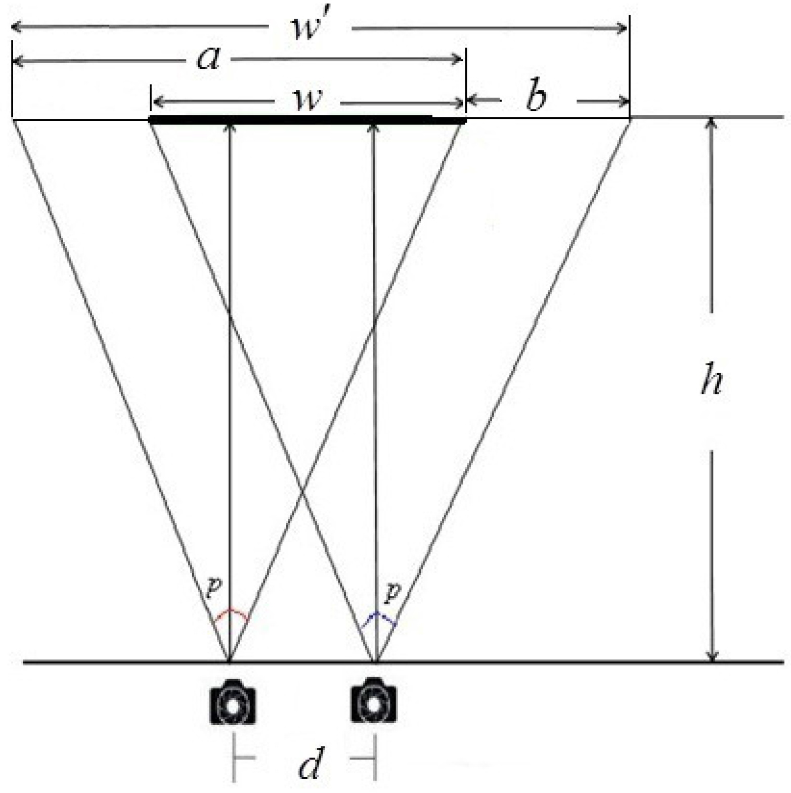
Binocular overlap percentage: The magnification of an image on the retina is
, as shown in
Figure 5 (here,
a is the original image width,
p is the viewing angle of the stereo camera,
is the viewing region of stereo camera and
w is the resulting composite image width, which denotes the binocular overlap of stereo camera).
can influence the values of positive and negative parallax and further affect the quality of the stereo images. In order to simplify the calculation,
was applied to the analysis on how binocular overlap affected stereoscopic capturing quality. Based on the geometric relations in
Figure 5, we can conclude:
Figure 5.
Schematic diagram of binocular overlap.
Figure 5.
Schematic diagram of binocular overlap.
For the sake of better understanding, the principle of the binocular overlap percentage was taken as the evaluation index. All test stereo images were divided into several different groups, each with a fixed value of
h and different values
d. Then, changing the value of
h and repeating the above experimental process, a series of stereoscopic image pairs was captured. Through subjective experiments, we took index
ξ as the binocular overlap percentage
in Equation (4) with the effort of Equation (5).
Based on a series of experiments, the binocular overlap percentage
ξ of stereoscopic image pairs can be calculated, and the range of
ξ is from 0.706–0.995. Through investigating the mapping between
ξ and the MOS value
, as shown in
Table 6, it can be used to evaluate the effect of the binocular overlap for long-distance shooting with the parallel camera configuration.
Table 6.
Mapping between ξ and the MOS value.
Table 6.
Mapping between ξ and the MOS value.
| Index: ξ |
|---|
| 5 | ξ≥0.955 |
| 4 | 0.943≤ξ<0.955 |
| 3 | 0.927≤ξ<0.943 |
| 2 | 0.899≤ξ<0.927 |
| 1 | ξ<0.899 |
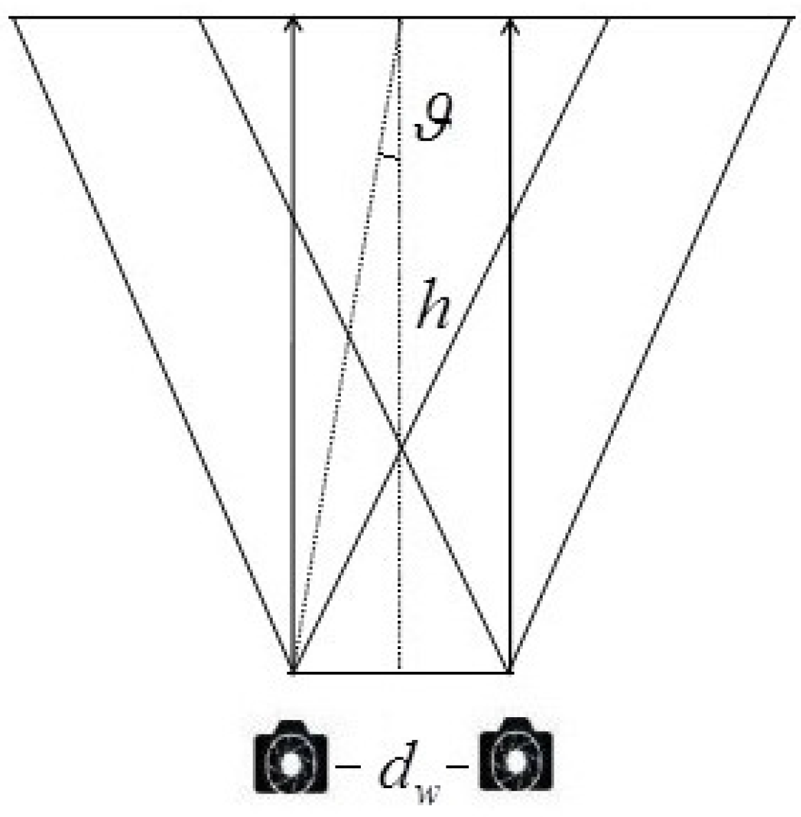
Camera visual acuity: Generally, the camera visual acuity is widely recognized as
(
ϑ; shown in
Figure 6). Let
h denote the shooting distance; the theoretical inter-camera distance
can be obtained (shown in Equation (6)) according to the camera visual acuity.
Figure 6.
Schematic diagram of camera visual acuity.
Figure 6.
Schematic diagram of camera visual acuity.
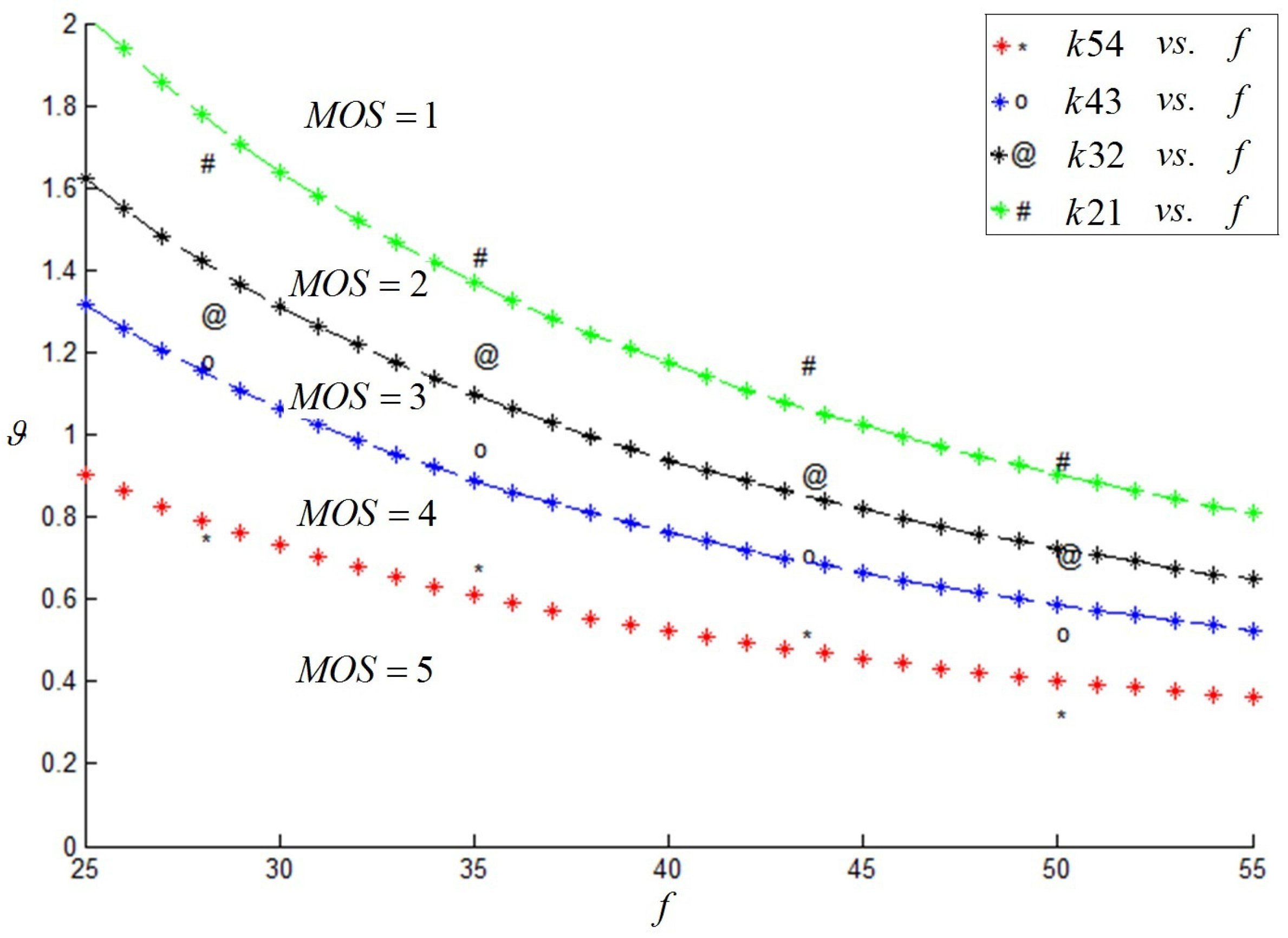
Figure 7.
Variation trend of ϑ(°) along with f (mm).
Figure 7.
Variation trend of ϑ(°) along with f (mm).
Over the long-distance shooting condition, the camera visual acuity was one of the main considerations. Ignoring this limitation might result in viewing discomfort or even the loss of stereo impression. In order to establish a five-level evaluation criterion, this paper took ϑ (shown in Equation (7)) as the evaluation index of camera visual acuity.
In order to enrich the experiments, several of the camera focal lengths
f were involved in our experiments; the experimental results are shown in
Figure 7, which indicated that
f, as well as
ϑ have a great effect on the subjective results. We proposed an ultimate assessment index
k, calculated from Equation (8). The mapping between
k and the MOS value,
, is shown in
Table 7. The values indicated that when
k was at most 55.98, a good stereoscopic effect could be obtained.
Table 7.
Mapping between k and the MOS value.
Table 7.
Mapping between k and the MOS value.
| Index: k |
|---|
| 5 | k≤38.41 |
| 4 | 38.41<k≤55.98 |
| 3 | 55.98<k≤60.00 |
| 2 | 60.00<k≤86.23 |
| 1 | k>86.23 |
Shape ratio of the parallel camera configuration: Similarly, the shooting principle of the shape ratio was applied to the parallel camera configuration. Based on a series of experiments, the value of
μ ranged from 0.095–0.932. Combined with the subjective experimental results, shown in
Table 8, the mapping between
μ and the MOS value,
, of stereoscopic image pairs had been investigated.
Table 8.
Mapping between μ and the MOS value.
Table 8.
Mapping between μ and the MOS value.
| Index: μ |
|---|
| 5 | μ≤0.120 |
| 4 | 0.120<μ≤0.147 |
| 3 | 0.147<μ≤0.201 |
| 2 | 0.201<μ≤0.226 |
| 1 | μ>0.226 |
4.3. Comprehensive Objective Evaluation Criteria
At present, the most common method used to integrate all independent individual factors into a global index is the linear weighting method [
43,
44,
45]. In order to reasonably evaluate the performance of the objective evaluation criteria, we applied a linear regression to the combination of the six factors, and each of them was given a weight. We specified
as the output value of the convergence rotation angle for the toed-in camera configuration,
as the output value of the shape ratio factor for the toed-in camera configuration,
as the output value of the modified 1/30 rule factor for the parallel camera configuration,
as the output value of the the binocular overlap percentage factor for the parallel camera configuration,
as the output value of the camera visual acuity factor for the parallel camera configuration and
as the value of the shape ratio factor for the parallel camera configuration. Considering that each of the factors had different properties in stereo capture, the establishment of the evaluation criteria should take all of the perspectives into account. Accordingly, they were regarded as individual factors that could be considered relatively independent. Although there may be a relation among the criteria, for simplicity, the global quality score
Q can be gained by using a linear combination of the criteria, which can be defined as:
where
denotes toed-in camera long-distance shooting,
denotes parallel camera long-distance shooting,
m,
n,
q,
r,
s and
t are weights of each factor in objective evaluation criteria and restricted by
and
.
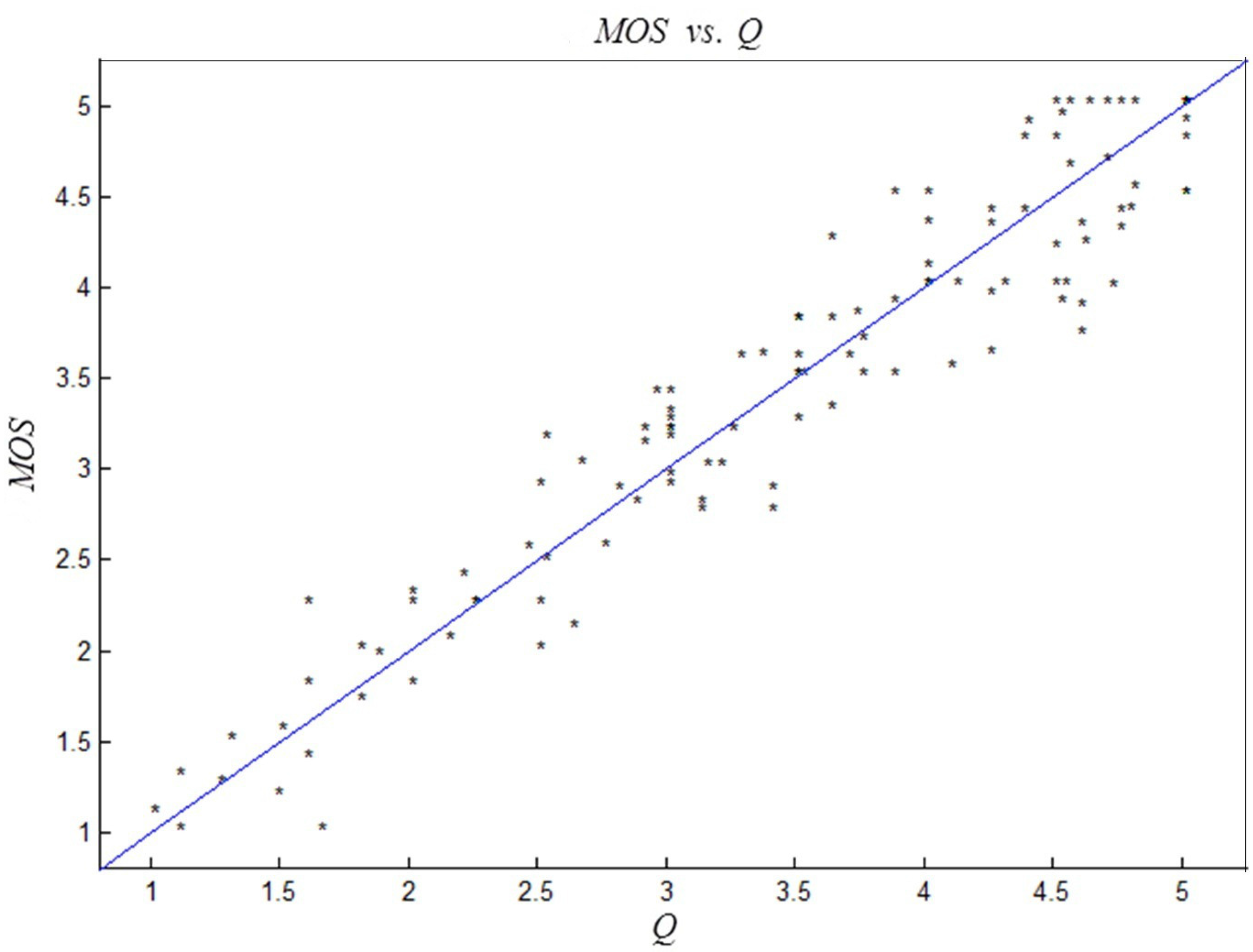
With the given weights of the factors, we can compute an objective score for each captured 3D image pair. At the same time, through a series of subjective tests, which has been done in
Section 2, the subjective score for each pair can also be obtained. In order to choose the proper values of the six weights, the correlation coefficients between the objective and subjective scores were computed on the whole database, and the corresponding values that achieved the max relativity were chosen for the weight of each factor. Based on the experimental results, the weights of each factor are shown in
Table 9. It is worth noting that the factors for each camera configuration get the same weight, indicating that the criteria proposed may have approximately the same importance in evaluating the performance of 3D capturing. However, the application of 3D capturing is a still a complex procedure, and more efforts are need.
Table 9.
Weights of each factor in the objective evaluation criteria.
Table 9.
Weights of each factor in the objective evaluation criteria.
| Shooting Type | m | n | q | r | s | t |
| , toed-in | 0.5 | 0.5 | 0 | 0 | 0 | 0 |
| , parallel | 0 | 0 | 0.25 | 0.25 | 0.25 | 0.25 |


