As we have discussed in the previous section, information about the movement of RT and OT is linked together in the features of the temporal trace via Equation (
4). We performed an extensive fitting procedure, to relate the position of the OT to the time interval
between the cusps of two subsequent sub-features. The foundations of this method have been presented in [
13]. Here, we radically improve it and correlate it with an analysis of the achievable precision in relation to the calibration stage. We will make use of the increased number and accuracy of the simulations and of the broader parameter space(see
Figure 2).
3.1. Numerical Approach
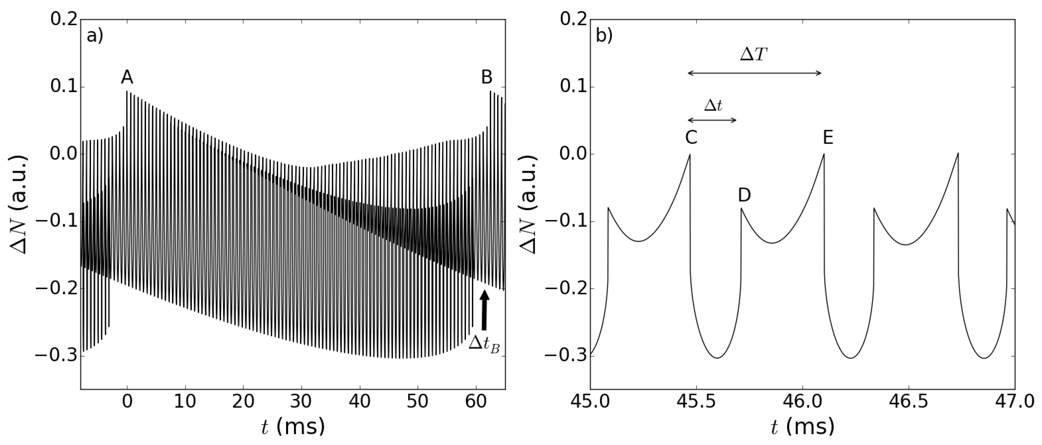
All of the simulations show that the sub-features emerge at the beginning of the slow fringe. Their duration
, when compared to the fast fringe duration
, is very small at the beginning, and it grows as the OT moves, until, near the end of the slow fringe, it becomes of the same magnitude as
. This actually results in the vanishing of the sub-features for a short period of time (indicated by
in
Figure 3a) that terminates at the slow fringe jump, after which they reappear in the next slow fringe; of course, the dynamical behavior of
across the slow fringe is complementary). We now illustrate how it is possible to relate the change in the time lapse
to the position of the OT. In our simulation, the OT velocity
is fixed, so we can define a “theoretical” position of the OT as given by the simple formula:
The time trace is thus sampled to extract the values of at different instants of time; at each time, we assume that the position of the OT is given by , and we will perform a best fit analysis to find a function that relates the position to . Since, as we mentioned above, there can be a short period across the slow fringe change in which the sub-features disappear, the fitting procedure can be performed in principle only along a single slow fringe. In the next subsection, we will tackle the problem of overcoming this limit, because an actual sensor must be capable of operating on an (ideally) arbitrarily long period, while at this stage, we will limit our analysis to a single slow fringe.
We have developed an algorithm capable of identifying and classifying (potentially in real time) all of the critical points of the temporal trace labeled in
Figure 3, so that we can register the time lapses between them. We set the origin of time at the first left cusp identified by the analysis algorithm, and we take the reference times
at each subsequent left cusp, while, as already mentioned before, we register the time lapse
that occurs between the right cusp of the
-th sub-feature and the left cusp of the
n-th one. Upon varying the fit on a broad basis of polynomial and transcendent functions, we found that a quadratic dependence works surprisingly well in approximating such dependence, and the candidate test function can be cast as:
The least squares method can be applied to evaluate the coefficients
for all of the simulations. Of course, coefficients
change for simulations at different
, because a larger
implies a reduced
and, thus,
. A proper interferometric sensor cannot suffer from such “reference arm” dependence, so the next step is to make the
dependence explicit in Equation (
6). For such a purpose, a new best fit procedure was carried out, resorting to the sets of simulations with varying
. The coefficients
and
have been found to have a quadratic and a linear dependence on
, respectively, while
is independent of
. The general formula we sought, which is supposed to hold for a wide range of the
plane, could then be cast as:
In this formula, we insert the solitary laser wavelength
to make the dimensions of the coefficients clear. To determine the parameters
from the entire set of simulations, we have evaluated the parameters
for all of the complete slow fringes in each simulation, and we have extracted the values of the
, along with their errors, by using their expressions as functions of the
. Each value obtained in this way has been treated as an independent detection of the “true”
value, so that its best estimate is the weighted means evaluated from all of the occurrences. We found:
and these parameters are constant within the assumptions described so far.
3.2. The Sensing Procedure: Methods, Sensitivity and Limits
Having obtained the relation defined in Equation (
7), it can be used to determine the displacement of the OT for any velocity pair
compatible with the limits of validity, which are going to be discussed here. First of all, the model was built on the stationary solutions of the LK equations, so we must ensure that the evolution of the target is adiabatic,
i.e., the laser system has enough time to reach a stationary state as the targets move. The slowest time on which the system evolves is of the order of tens of nanoseconds [
2,
3], while the evolution timescale of the carrier density difference associated with the motion of the RT is of the order of the fast fringe period,
. Therefore, adiabaticity requires that
with
m/s. In our simulations, the maximum value for the RT velocity was thus set to 5 m/s.
The reliability of the phenomenological relation Equation (
6) can be assessed by appreciation of the normalized root mean square deviation for each fitting procedure:
where
is the number of sub-features identified by the algorithm. We observed that its value was very small (of the order of a few
) as long as the ratio
was well above
. Near this threshold, it jumped abruptly to values of the order of
, thus indicating that the assumption of a quadratic dependence is no longer valid. In order to be conservative, in the evaluation of the parameters
in Equation (
8), we have used only simulations with
. The smallest displacement that can be observed depends on the time between two subsequent observations of
, which is of the order of the fast fringe periodicity,
, so that, in principle,
Since, as we discussed above, the sensing procedure allows
, the scheme we are proposing should be capable of reaching a sensitivity of
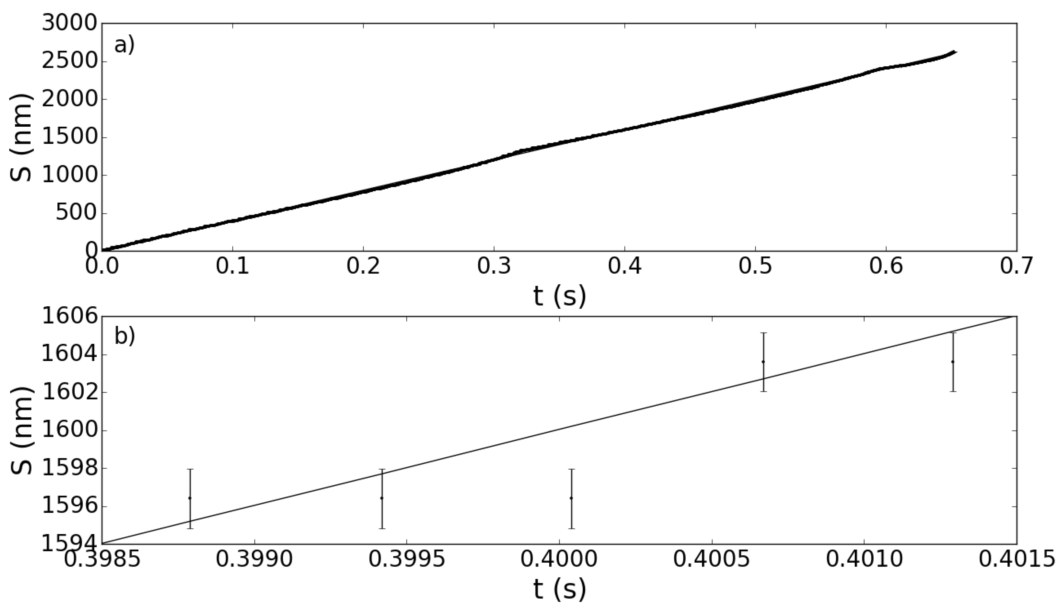
, which is of order of a few nanometers. An example of the results that can be obtained with the sensing procedure described so far is given in
Figure 5.
Figure 5.
Plot of the position of the object target (OT) target
versus time, for a simulation with
m/s and
m/s. The other parameters are as in
Figure 3. The solid line represents the theoretical position
(see Equation (
5)). The dots mark the position
as predicted by the phenomenological Equation (
7) and the associated errors
as given by Equation (
11). (
a) The representation over the entire period of a slow fringe; (
b) a close-up in which the accuracy of
in retrieving
can be appreciated.
It is evident by inspection of the close-up,
Figure 5b, that the potential measurements of the OT are well within the 10-nm deviation from the theoretically-expected values (the solid line). Of course, this result depends crucially on the accuracy in determining the coefficients
of Equation (
8). In fact, we can assume that the error on the determination on the OT displacement due to uncertainties in the
parameters is given by applying the error propagation law to the phenomenological Equation (
7):
and this error must be smaller than the expected sensitivity given by Equation (
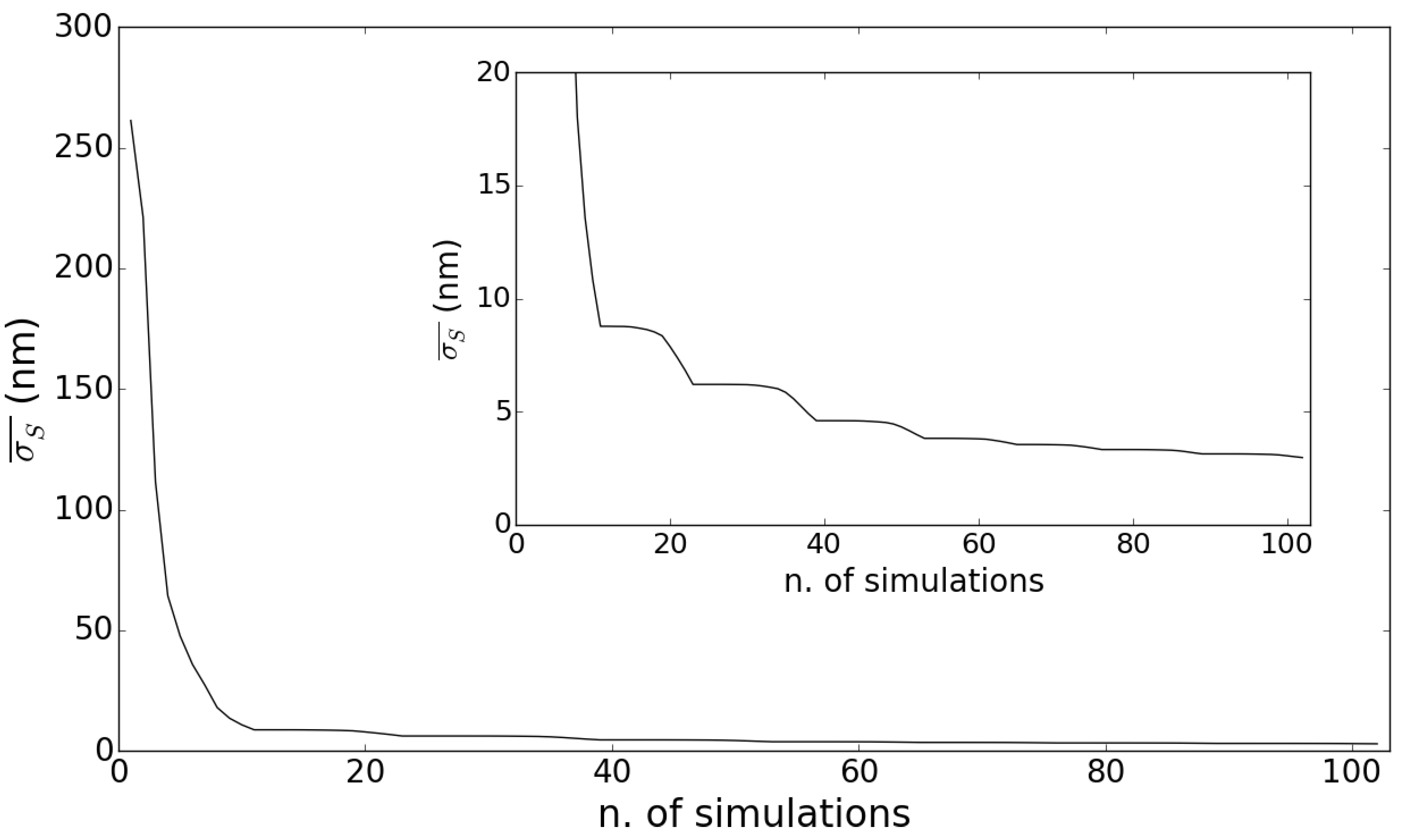
10). Increasing the number of simulated slow fringes, on which the determination of the
parameters is performed, will result in better accuracy. To check this, we have evaluated the mean error
as a function of the number of simulations. The result is shown in
Figure 6.
As we can see, the curve falls quite rapidly below 10 nm and then tends to saturate around 5 nm. This confirms that the
parameters can be evaluated with sufficient precision for our sensing scheme to reach nanometric sensitivity. The values reported in Equation (
8) have been obtained using a set of 100 simulated slow fringes.
Figure 6.
Plot of the mean error on the determination of the OT position () as a function of the number of simulations used to determine the coefficients. The inset focuses on the relevant range of values for and shows that it actually reaches the nanometer range.
Figure 6.
Plot of the mean error on the determination of the OT position () as a function of the number of simulations used to determine the coefficients. The inset focuses on the relevant range of values for and shows that it actually reaches the nanometer range.
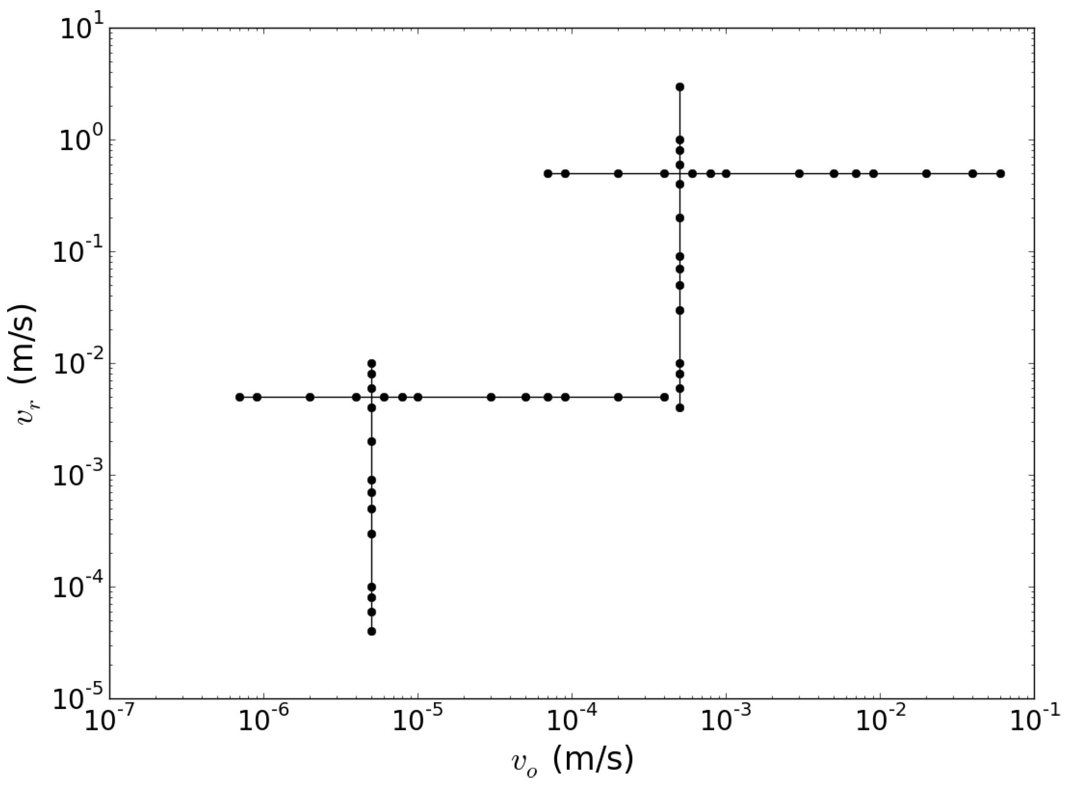
In a realistic sensor, the determination of the
parameters and their uncertainties is based on a calibration procedure where targets with known velocities are employed. The calibration should be performed for a set of pairs
conveniently distributed in the parameter space according to the guidelines discussed in the first part of this subsection. This calibration needs to be done only once, since the parameters determined in this way should remain valid for a range of at least three orders of magnitude in both target velocities. The number of calibration runs determines the accuracy of the value obtained for the
parameters and, consequently, the sensitivity of the device. A curve representing the error on the determination of the position of the target as a function of the numbers of calibration runs should have the behavior reported in
Figure 6, but other factors related to the experimental conditions may hinder the capability of achieving the predicted nanometric sensitivity. Just as an example, mechanical vibrations of the set-up, irregularities in the motion provided by the step motor driving the RT and/or OT and current fluctuations in the power supply of the laser are all obvious sources of errors in the measure. While such sources can be tamed in principle, we will consider the effect of a more intrinsic limitation in
Section 3.4.
Another issue to be addressed is how to circumvent the detection limitation to a single slow fringe due to the disappearance of the sub-feature discussed above. Our simulations proved that the number of fast fringes not exhibiting a sub-feature occurs invariably at the end of a slow fringe, and it decreases with increasing feedback strengths
and
. In any case, in the time lapse
, our algorithm is “blind” to the target motion. A sufficiently high feedback should limit this interval to a small fraction of the slow fringe period, and during this period, the OT displacement can be extrapolated via the simple formula
, where
is the last detected OT velocity, just before sub-feature disappearance. This simple method has been experimentally tested in [
13] and proven to be sufficiently accurate within experimental uncertainties. In the next subsection, we will discuss in detail this and other aspects of the sensing procedure related to the feedback level.
Finally, let us stress that, in principle, the sensitivity could be pushed further beyond, since the limiting ratio
is set by the failure of the quadratic fit proposed in Equation (
7). For lower values, new sets of simulations and a more refined fitting procedure might yield a reliable relation
. In any case, the necessity to detect a sufficient number of slow fringes and of densely sampling each fast fringe might increase the requirement in terms of bandwidth and the buffer memory of the electronics reading out the voltage at the QCL contacts.
3.3. The Role of the Feedback Parameters in the Sensing Scheme
As was shown in
Section 2.1, the key element for the sensor proposed in this work is the high feedback level, which ensures, in the spectral domain, the nonlinear frequency coupling and, in the time domain, the appearance of the sub-features, whence our algorithm extracts the information of the OT motion with nanometric accuracy. We stress that this feature is critical of the nonlinear dynamics of the laser in providing the coupling and of the QCL in particular, since this emitter can sustain large feedback without entering chaotic regimes [
2]. We will now illustrate in some detail the role of the feedback strength on the system dynamics.
We analyzed the system behavior when the feedback levels
and
are changed, while keeping the ratio
fixed. The values of the target velocities were set to
m/s and
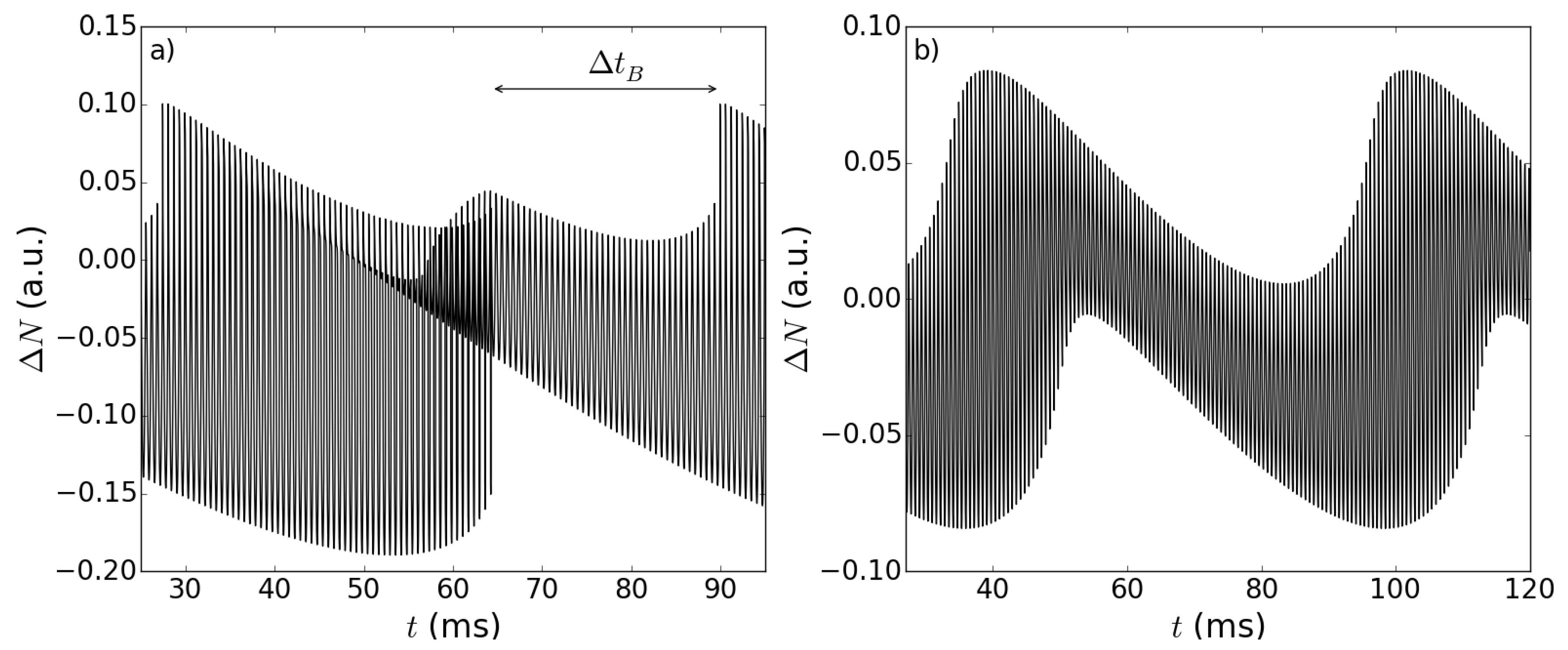
m/s. Decreasing the feedback results in a reduction of the time fraction of the slow fringe in which the sub-features are present, as it is possible to see in
Figure 7a. At even lower feedback levels, the sub-features disappear completely, as shown in
Figure 7b.
Figure 7.
Plot of
for two different levels of feedback with fixed ratio
. The other parameters are as in
Figure 3. (
a) The feedback values are
and
. Notice that the sub-features are present only in (approximatively) the second half of the slow fringe, as indicated by the time lapse
. The temporal trace (
b), obtained using
and
, has no sub-features at all.
On the contrary, as the feedback parameters increase, new temporal features appear in the fast fringes, in the form of additional pairs of cusps with even shorter duration (see
Figure 8a). While such “sub-sub-features” may be the subject of further investigations to enhance even further the potential sensitivity of our scheme, another interesting insight for this phenomenon can be gathered from inspecting the Fourier transform of
for different values of the feedback parameters.
Figure 8.
Plot of
as a function of
t (
a,
c) along with their corresponding Fourier transforms plotted in a log-log plane (
b,
d); upper part:
; lower part:
. The ratio
remains fixed. The other parameters are as in
Figure 3.
Figure 8.
Plot of
as a function of
t (
a,
c) along with their corresponding Fourier transforms plotted in a log-log plane (
b,
d); upper part:
; lower part:
. The ratio
remains fixed. The other parameters are as in
Figure 3.
Figure
Figure 8b shows the Fourier transform of the temporal trace corresponding to
Figure 8a. One observes a strong peak at the lowest frequency
and its higher harmonics, while at higher frequencies, as in the case of
Figure 4, the main peak occurs at the frequency difference
. Remarkably, there are several higher harmonics of this dominant note, whose peaks decrease in intensity with a power law, indicating once again the strong nonlinear character of the interaction, brought about by the laser dynamics. Interestingly, the time trace is still regularly periodic in this case, although the peak pattern is complicated by the appearance of the new cusps. Upon further increase of the feedback strength, we observe (see
Figure 8d) that the background increases considerably, while the peaks at the dominant frequencies become more intense and do not decrease linearly any more; accordingly, the time trace (see
Figure 8c) still exhibits regular, though complex features on the short time scale, while at longer timescales, comparable with the slow fringe period, it appears irregular, and we cannot expect to recover a relation formally similar to Equation (
7).
Summing up, as concerns the proposed sensing scheme, in the general dynamical scenario of the retro-injected QCL, the most suitable feedback level one should try to set as the operational point for the sensor is the one close to the threshold of the appearance of the sub-sub-features. In this condition, in fact, the time lapse in which the sub-features disappear is the shortest possible, thus reducing the error implied by the extrapolation procedure described above.
3.4. Influence of the QCL Linewidth on the Sensitivity
As we mentioned in
Section 3.2, several other sources of error may worsen the accuracy of Equation (
7), as given by the errors on its coefficients in Equation (
8), which are solely determined by the sample set on which the calibration is performed. We consider now the effect of the finite linewidth of the QCL emission. The latter is associated with phase variation induced by spontaneous emission, carrier-induced refractive index change and injection current fluctuations [
16,
17]. Moreover, it is known that the presence of optical feedback leads to linewidth broadening or narrowing depending on the external cavity phase shift [
18]. A rigorous theoretical approach that describes all of these phenomena would consist of adding Langevin noise sources in the LK Equations (
1) and (
2), as is described in [
17]. Here, in order to provide a simple estimation of the role of the QCL linewidth in limiting the proposed sensor accuracy, we suppose that the stochastic fluctuations of the free running laser frequency, denoted now as
, which follows a normal distribution centered in
with amplitude
, affect the frequency
of the reinjected QCL trough Equation (
3) and, in turn, the values of
as given by Equation (
4). We can thus expect the fringe jumps and the sub-feature duration to fluctuate accordingly; this will induce additional uncertainties in the determination of the target displacement as evaluated in Equation (
7). In an ergodic hypothesis, we consider the ensemble average of a large number of simulations with fixed
as representative of the time average in the temporal evolution of fluctuating variables, as provided by the integration of Equations (
1) and (
2) with the inclusion of Langevin noise sources [
17].
In particular, for the study case
m/s and
m/s and for values of
ranging from 100 kHz to 10 MHz, which are in agreement with estimations reported in recent literature [
19,
20,
21], a set of 50 determinations of
was randomly generated and used to obtain 50
traces, via Equation (
3) (where, of course,
was replaced by
). The immediate visual effect of the
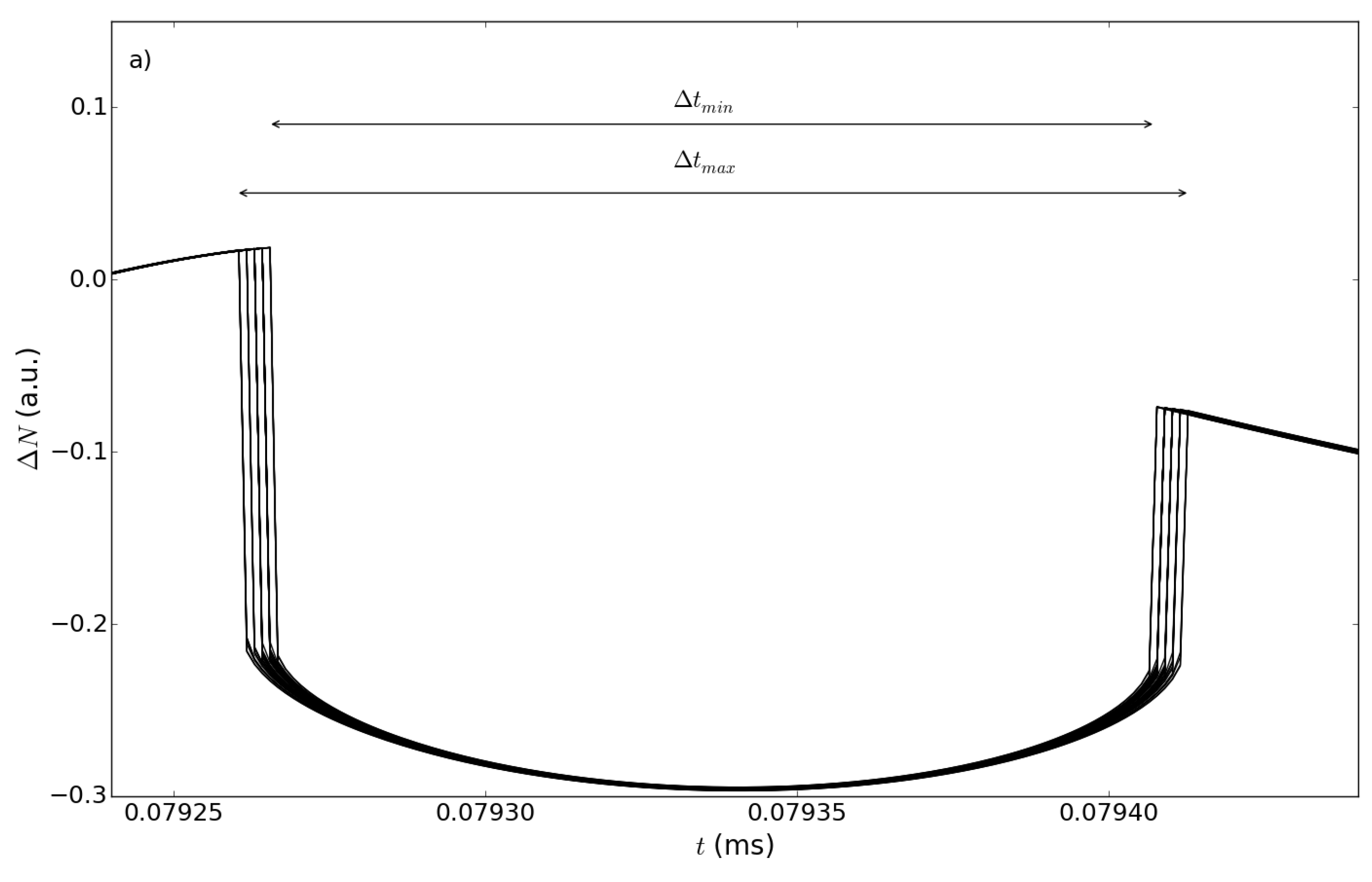
fluctuations introduced in this way is the jittering of the cusps delimiting the sub-features (see
Figure 9). This amounts to saying that one can detect a set of
, corresponding to left cusps initiating a sub-feature, and another set
, corresponding to right cusps ending a sub-feature (see
Figure 3b), which define a
array of detectable sub-feature time lapses
. Indicated as
and
, the maximum and minimum values of
, respectively (see
Figure 9), the dispersion
is considered as the error on the determination of
induced by the finite linewidth.
The uncertainty on the OT position has been derived with the error propagation law:
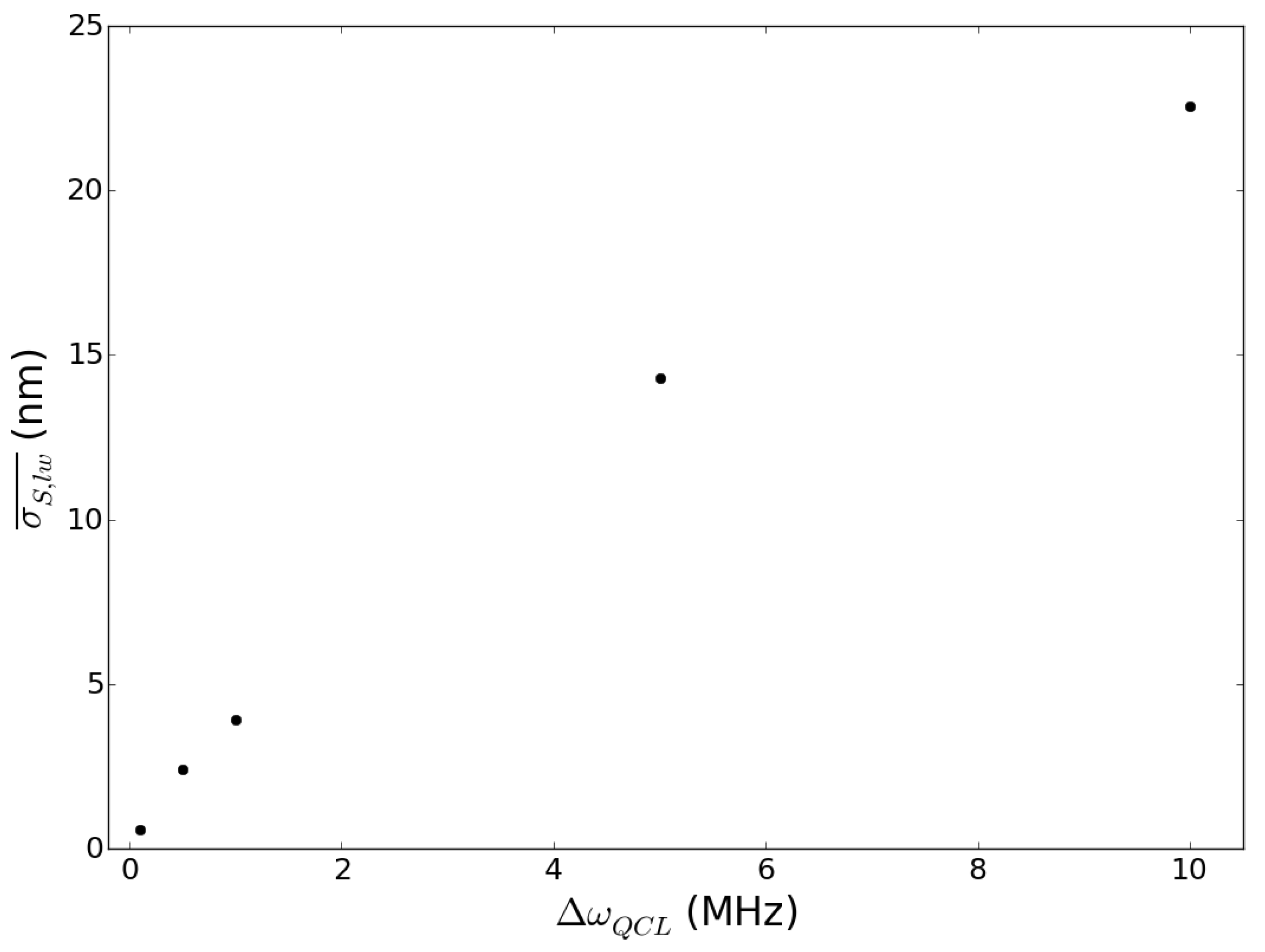
In
Figure 10, we represent the behavior of the mean error
(obtained by averaging
over the set of sub-features considered) as a function of the QCL linewidth. As we can see, the errors grow with linewidth according to a power law, and for
MHz, they are below 10 nm, thus comparable to those intrinsic to our deterministic method.
Figure 9.
Broadening of the temporal trace
for a linewidth
MHz. The plot focuses on the time lapse between two consequent sub-features, showing the maximum (
) and the minimum (
) values of
considered in the evaluation of the uncertainty
. The other parameters are as in
Figure 3.
Figure 9.
Broadening of the temporal trace
for a linewidth
MHz. The plot focuses on the time lapse between two consequent sub-features, showing the maximum (
) and the minimum (
) values of
considered in the evaluation of the uncertainty
. The other parameters are as in
Figure 3.
Figure 10.
Plot of the uncertainty against the quantum cascade laser (QCL) linewidth associated here with quantity .
Figure 10.
Plot of the uncertainty against the quantum cascade laser (QCL) linewidth associated here with quantity .


