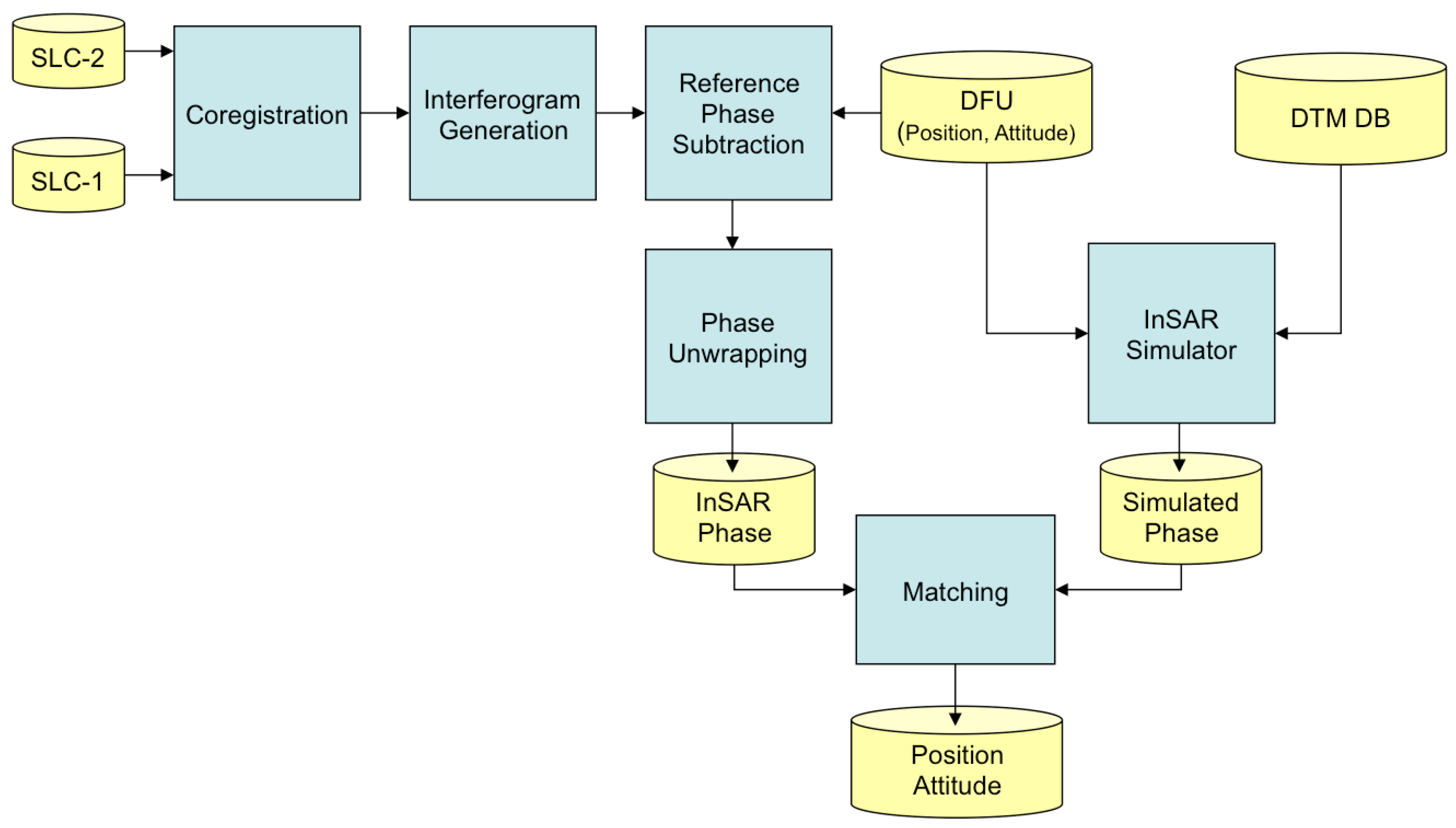
2.2. Basic Concepts and Geo-Referencing Procedure
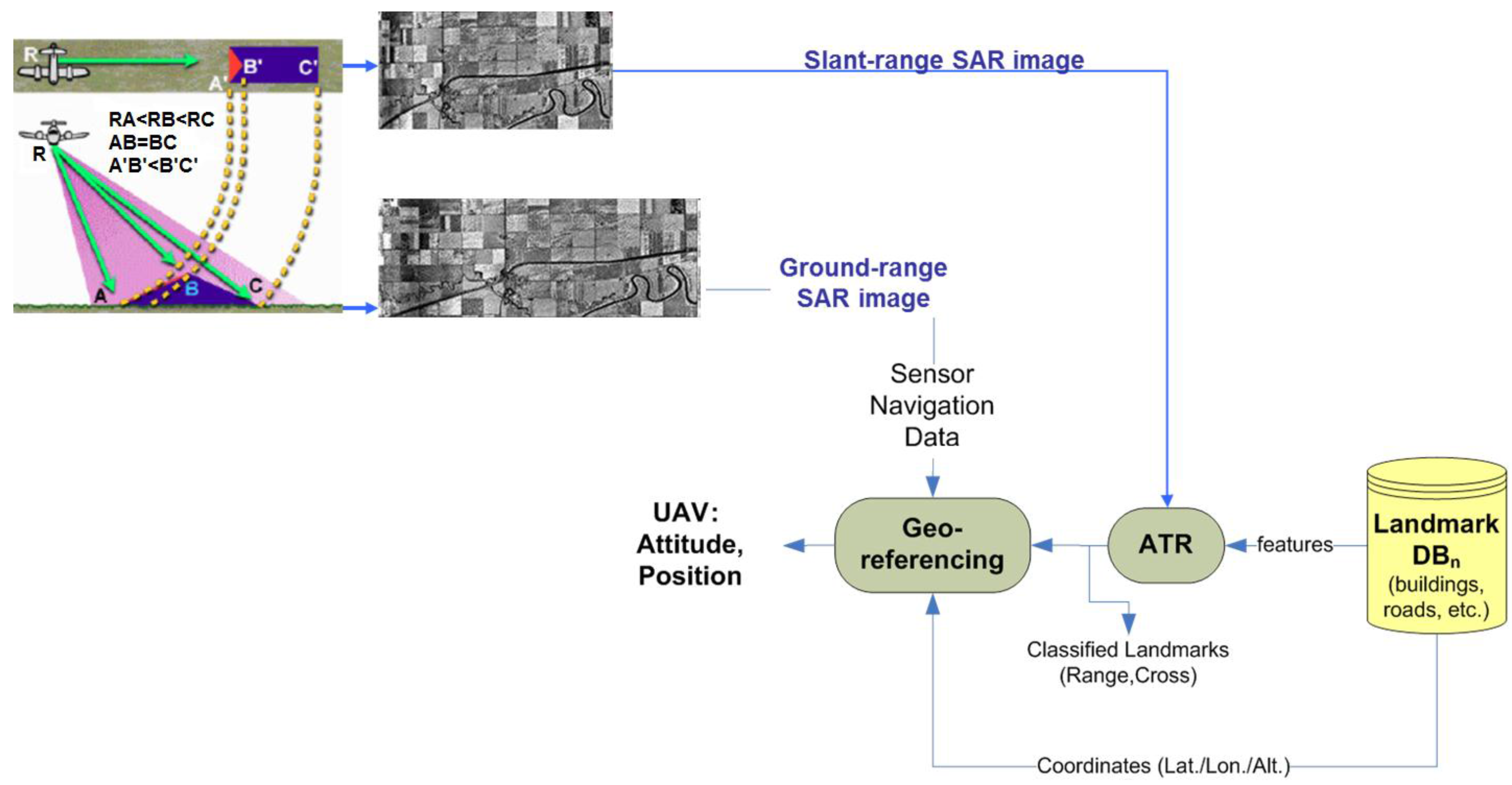
The whole (SAR amplitude-based) geo-referencing procedure is depicted in the processing-flow in
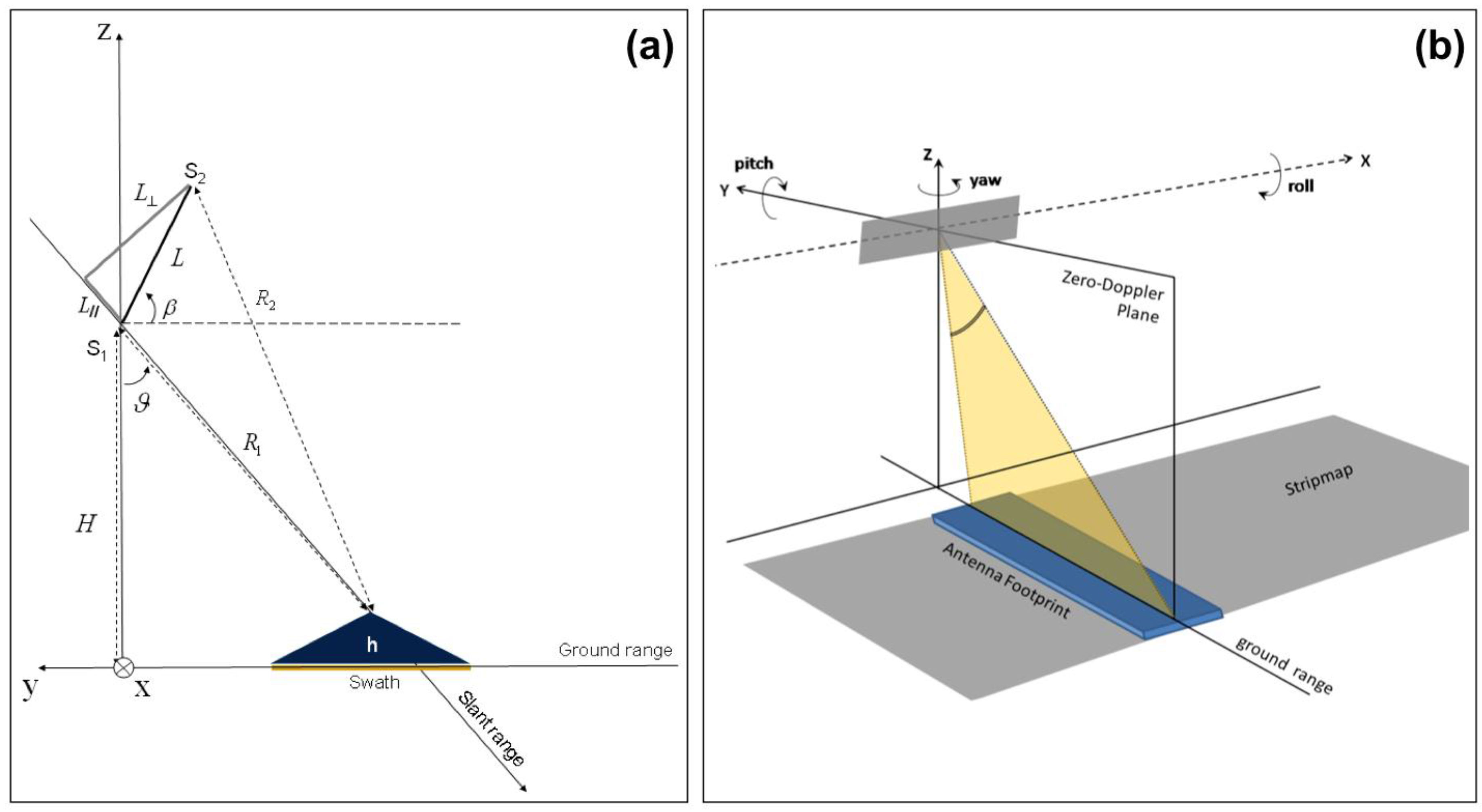
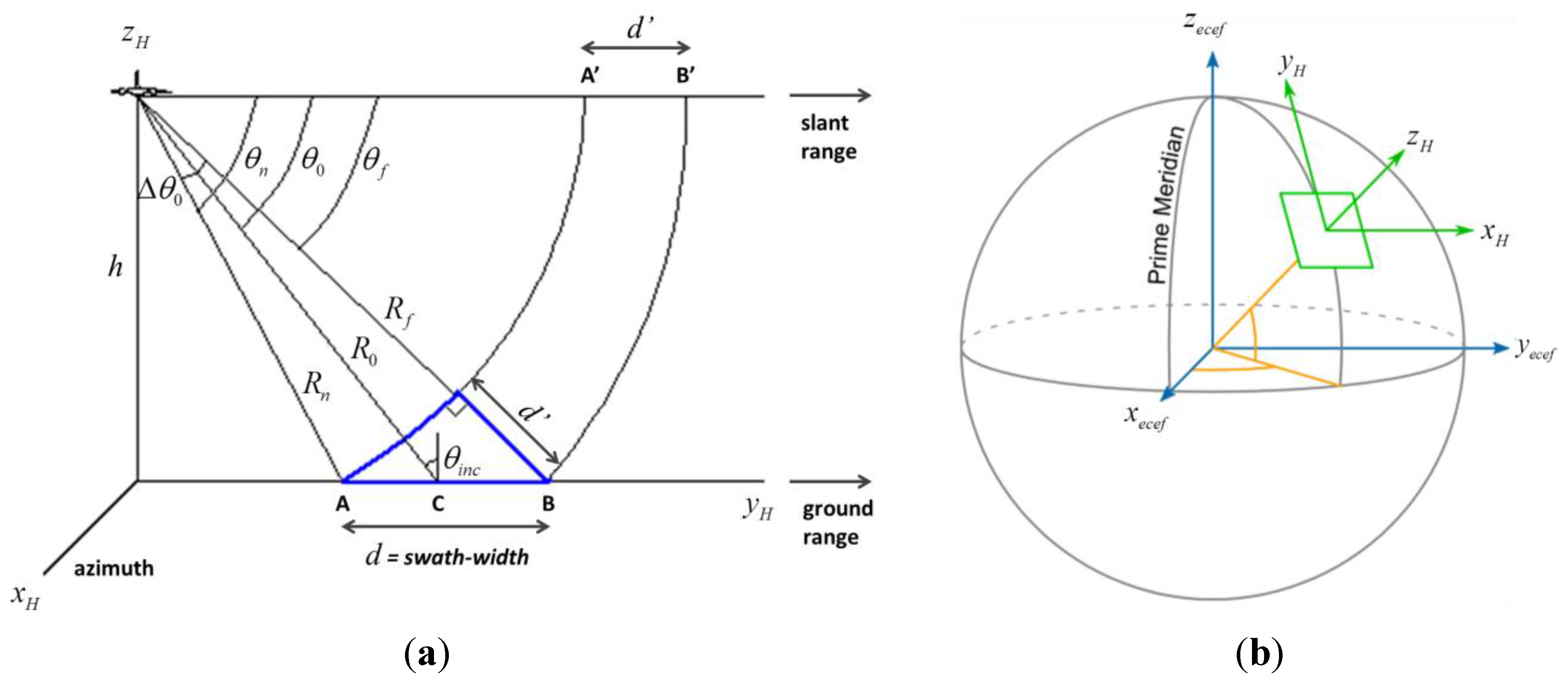
Figure 1. It can be noted that viewing geometry and SAR geometrical distortions have to be considered in order to derive a meaningful geo-referencing algorithm based on the recognition of landmarks in SAR images. A basic viewing geometry of an SAR is shown in
Figure 2a [
8]: a platform flying with a given velocity at altitude
h carries a
side-looking radar antenna that illuminates the Earth’s surface with pulses of electromagnetic radiation. The direction of travel of the platform is known as the
azimuth direction, while the distance from the radar track is measured in the
slant range direction. The
ground range and its dependence on the angle
θ is also depicted. Note that in
Figure 2b we assumed the flat Earth approximation, which can be considered valid for the airborne case, even for long-range systems [
11]. Before presenting the proposed procedure, we introduce some quantities that will be used in the following. A complete list can be found in
Table 1.
Inertial system of coordinates: classically, it is the Cartesian system of coordinates. In the geodetic literature, an inertial system is an Earth-Centred-Earth-Fixed (ECEF) frame where the origin is at the Earth’s centre of mass, the (
xecef,
yecef) plane coincides with the equatorial plane, and the (
xecef,
zecef) plane contains the first meridian) [
12].
Local flat Earth: position of a point
can be computed from a geodetic latitude-longitude-altitude frame or an ECEF frame by assuming that the flat Earth
zH-axis is normal to the Earth only at the initial geodetic coordinates [
13]. For our application, the flat Earth model can be assumed if
h <<
RE = 6370 km, where
RE is the Earth radius and
h is the SAR (or aircraft) altitude [
11]. As a consequence, the coordinates for a specific ellipsoid planet can be easily computed resorting to commercial software tool, such as in [
14]. A pictorial view of ECEF and flat Earth (
H) frame can be found in
Figure 2b.
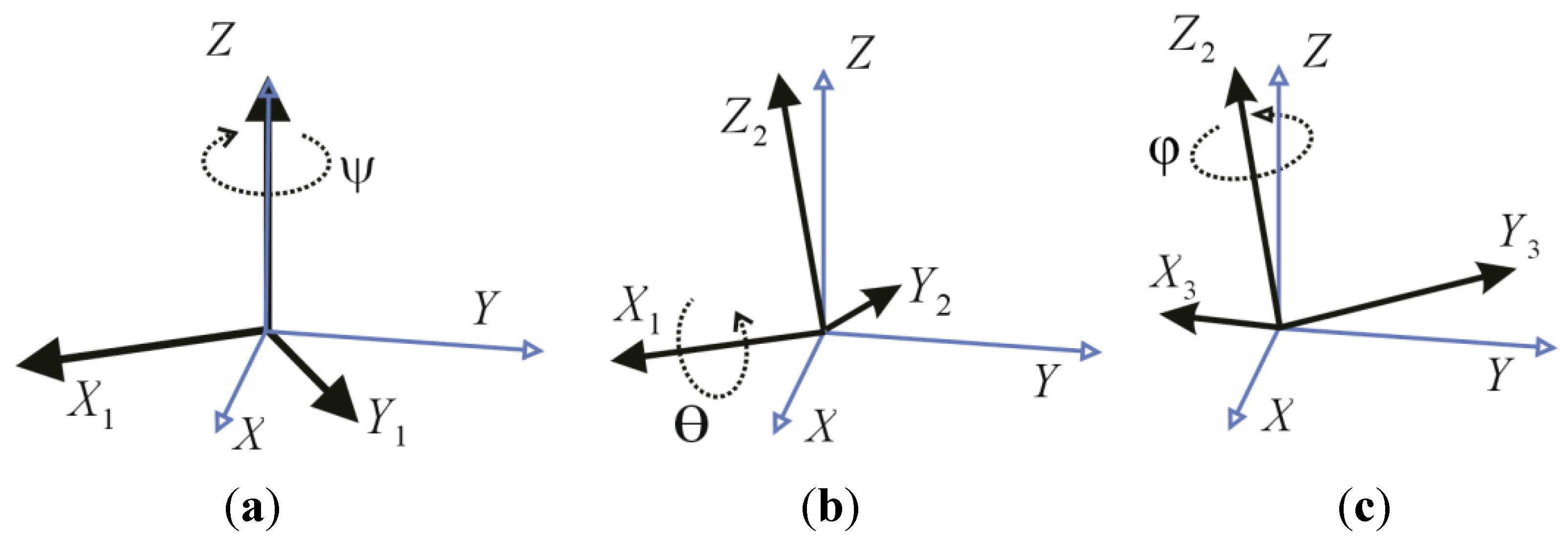
Euler angles: angles that are used to define the orientation of a rigid body within an inertial system of coordinates [
15] (see
Figure 3). Such angles hereinafter will be also referred as attitude
.
Now, let us define a coordinate transformation of a point
from an inertial (
H) frame to a new coordinate system (
C) [
15,
16]:
where every quantity is defined in
Table 1. This transformation has some interesting properties [
15]: if the ground was planar (
), the transformation would be
affine;
can be factorized into the product of three orthonormal-rotation-matrices; a parallel pair in the
H domain remains parallel in
C; the transformation either stretches or shrinks a vector; typical SAR distortions (
i.e.,
foreshortening,
layover,
shadow in
Figure 1 and in
Figure 2a) are correctly modelled [
16,
17].
Equation (1) can be inverted as follows:
where every quantity is defined in
Table 1. The main geometrical properties considered here are: invariance to rotation of an SAR image with respect to its corresponding geographical map; invariance to scale factor (stretch or shrink); invariance to translation; invariance to slant range, foreshortening and layover distortions for
(
Figure 2b). To perform the feasibility analysis of the SAR amplitude-based geo-referencing approach, we propose a procedure relying on a well-established and simple coordinate transformation of a point from an inertial frame (
H) to a new coordinate system (
C), hereinafter the radar frame [
16]. Equation (1) allows us to transform three-coordinates of the local flat Earth (
H) frame into three-coordinates of the system (
C). However, our goal is to transform a 3-coordinate system into a new two-coordinate system, where every point is a pixel of the scene imaged by the SAR. As a consequence, for the third coordinate the following condition holds:
Note that,
can be still computed as a function of the focal length for an optical image, but it cannot be generally derived for a SAR image if
,
and
are unknown.
By exploiting Equations (1) and (2), the following relation for the aircraft position (or equivalently the SAR position) estimation can be written:
where it
was set equal to one. The previous equation clearly states that SAR position (
) can be found if and only if: SAR attitude
is “correctly” measured or estimated; coordinates of a point landmark (
) are known (from a DB) in the inertial coordinate system
H; the same landmark point is imaged by the SAR and its coordinates in the non-inertial coordinate system
C,
i.e.,
, are correctly extracted by the ATR processing chain.
Thus, SAR position can be computed by re-writing Equation (4) as follows:
An SAR sensor essentially measures the slant-range between the sensor position
and a GCP, e.g.,:
, point A in
Figure 2a located at the near range
Rn and corresponding to a SAR attitude (
ψ = 0°,
θ = θn,
φ = 0°). Thus, if the GCP is in the landmark DB (
i.e.,
is known) and is correctly extracted from the SAR image by the ATR chain (
i.e.,
is known), then the SAR sensor position
can be retrieved by using Equation (5). Note also that (
ψ,
θn, φ) have to be estimated or measured in order to exploit Equation (5).
It is worth noting that this section does not aim to provide an SAR-amplitude based geo-referencing procedure, but only a simplified mathematical approach to perform a feasibility analysis.
Table 1.
Parameter classification, definition and measurement unit.
Table 1.
Parameter classification, definition and measurement unit.
| | Parameter | Definition | Measurement Unit |
|---|
| Coordinate Systems | H | Local flat Earth coordinate system in Figure 2b | – |
| C | Local coordinate system, e.g., radar coordinates | – |
| h | Altitude respect to frame H in Figure 2a | (km) |
| Position of a point in the H frame in Figure 2b, e.g., SAR or GCP () | (m) |
| Translation vector (3 × 1) in the H frame | (m) |
| Scale parameter of the transformation from H to C | – |
| Rotation matrix (3 × 3) from H to C frame | – |
| Position of a point in the C frame (e.g., GCP position ) | (m) |
| Translation vector (3 × 1) in the C frame | (m) |
| Scale parameter of the transformation from C to H | – |
| Rotation matrix (3 × 3) from C to H frame | – |
| H frame coordinates of SAR/aircraft, point A, C and B in Figure 2a | (m) |
| (ψ, θ, φ) | Euler angles in Figure 3 | (°) |
| Radar | θ0 | Depression angle of radar beam-centre in Figure 2a | (°) |
| θinc = 90° − θ0 | Incidence angle of radar beam-centre on a locally flat surface in
Figure 2a | (°) |
| d | Swath-width in Figure 2a | (km) |
| Δθ0 | Beam-width in the elevation plane in Figure 2a | (°) |
| Δr , Δcr | Image resolution along range and cross-range | (m) |
| Rn, R0, Rf | Near, center of the beam and far range in Figure 2a | (km) |
| Rmax or Rf | Maximum detection range (or far range) | (km) |
| θn, θ0, θf | Near, center of the beam and far depression angle in Figure 2a | (°) |
| Navigation | | RALT accuracy in [%] (root mean square error—rmse) | – |
| IMU attitude accuracy on each component (rmse) | (°) |
| Processing | | Inaccuracy on landmark position extraction from a SAR image | (pixel) |
Figure 2.
(a) Airborne side looking SAR geometry; (b) Basic flat-Earth geometry.
Figure 2.
(a) Airborne side looking SAR geometry; (b) Basic flat-Earth geometry.
Figure 3.
(a) Euler angles (ψ, θ, φ): (a) ψ defines the first rotation about the z-axis (note that the angle ψ in the figure is negative); (b) θ defines the second rotation about the x1-axis (note that θ is negative); (c) φ defines the third rotation about the z2-axis (note that φ is positive).
Figure 3.
(a) Euler angles (ψ, θ, φ): (a) ψ defines the first rotation about the z-axis (note that the angle ψ in the figure is negative); (b) θ defines the second rotation about the x1-axis (note that θ is negative); (c) φ defines the third rotation about the z2-axis (note that φ is positive).
2.3. Feasibility Analysis
As already stated in
Section 1, the feasibility analysis refers in particular to MALE UAV class [
10], which permits heavy and wide payloads to be carried onboard, and can be affected by a dramatic cumulative drift during long mission when GPS data are not reliable. Some examples of MALE UAVs are Predator B, Global Hawk and Gray Eagle, which are actually equipped with SAR system and can be also equipped with InSAR system (more details in
Section 3). Several competing system parameters have to be considered in the feasibility analysis as detailed in the following.
X band choice is mainly driven by both the limited payload offered by X-band SAR/InSAR systems and by the wavelength robustness to “rain fading” [
17].
Concerning the polarisation, a single channel leads to a small and light SAR system that can fit onboard a UAV. Moreover, in the case of single polarisation, well-suited statistical distribution for terrain modelling can be employed by a fast and high-performance ATR chain. Finally, backscattering in VV polarization is higher than in HH polarisation for incidence angle greater than 50° and X band [
17].
SAR image resolution has to be chosen as a trade-off among competing requirements. Range/cross-range resolution of about 1 m is suitable for recognizing terrain landmarks,
i.e., large targets such as buildings, cross-roads, whose shorter linear dimension is at least 10–20 times the suggested resolution [
18]. On the contrary, pixel resolution higher than 1m would be unnecessary and increase ATR computational load.
Stripmap imaging mode allows us a shorter observation/integration time (as opposed to spotlight mode), lower computational complexity, and easier autofocusing [
19]; moreover, it also requires a mechanical antenna steering mechanism simpler and lighter than other imaging modes [
18].
Requirements on SAR acquisition geometry (
i.e., altitude
h and attitude (
ψ,
θ,
φ)), IMU attitude measurement, SAR swath-width, landmark characteristics, ATR accuracy, and operative scenarios, were derived through Montecarlo simulations according to the procedure described in
Section 2.1.
In particular, the simulated scenarios assume good position accuracy on landmark coordinates derived by ATR chain, while exploring the various parameters in
Section 2.2 to achieve the “best” aircraft position estimates through the SAR-amplitude based approach.
Table 2 reports a résumé of the specific case studies presented in the following.
The swath-width
d is defined by the near-range
Rn and the far-range
Rf reported in
Table 2 for all the explored configurations. Position estimation is based on a single GCP and computed in three cases: point A (
i.e.,
), C (
i.e.,
) and B (
i.e.,
) in
Figure 2a and in
Table 2.
Table 2.
Synthetic aperture radar (SAR) amplitudes-based approach: common parameter settings, case studies and results.
Table 2.
Synthetic aperture radar (SAR) amplitudes-based approach: common parameter settings, case studies and results.
| | SAR | Coordinates (SAR, GCPs) and Route | Source of Inaccuracy |
|---|
| Common Parameters of Case Studies | VV polarization
X band
Stripmap mode
Δr = Δcr = 1 m | , |
Δh = 0.5%, 1%, 2%
Δp = ±2, ±4 |
| , |
| , |
| , |
|
| Case Study | SAR/Platform Position (m) | Other Settings (km) | SAR Position Estimates |
| CS#1 | | | Figure 4: accuracy lower than in CS#2–5, = 10° |
| CS#2 | | | Figure 5: = 30° |
| CS#3 | | Figure 6: accuracy lower than in CS#2, = 40° |
| CS#4 | | | Figure 7: = 30° |
| CS#5 | | Figure 8: accuracy lower than in CS#4, = 40° |
We assumed that: SAR attitude (
ψ,
θ,
φ) is measured by the IMU with a rmse ranging from 0.05° to 1° (without GPS correction), which is allowed by high accurate (
i.e., navigation grade class) commercial IMU such as LN-100G IMU [
20];
h is measured by a RALT with accuracy equal to Δ
h = 0.5%, 1%, 2%, which is allowed by commercial systems compliant with the regulation in [
21]; SAR image resolution is Δ
r = Δ
cr = 1 m; inaccuracy on landmark position extraction in SAR image is Δ
p = ±2, ±4 pixels, which is compatible with the performance of the ATR algorithms [
5,
8]. Finally, without loss of generality, we refer to the simplified geometry in
Figure 2a defined by the following relations:
,
ψ = 0°,
φ = 0°.
The first case study (CS#1 in
Table 2) corresponds to a high altitude flight (
i.e.,
h = 8 km), which is allowed by a MALE UAV class [
10].
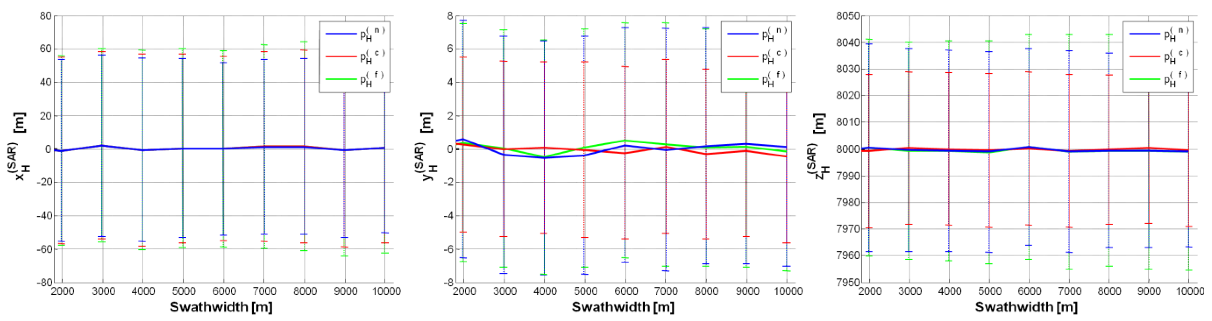
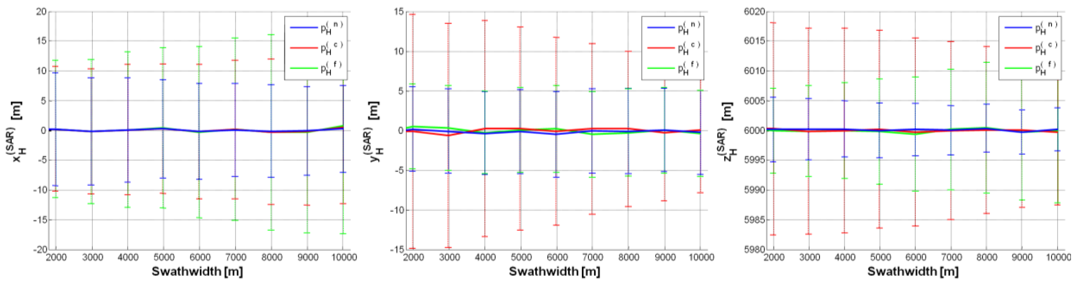
Figure 4 depicts UAV/SAR position estimates under the “best” configuration (
i.e.,
θ0 = 10°,
, Δ
h = 0.5%, Δ
p = ±2), with error bars proportional to the error standard deviation (std): no significant bias can be noted, but the std, which is very stable w.r.t. the swath-width, is too large on the 1st and 3rd component (
). Even by increasing
θ0 (from 10° to 40°), suitable results cannot be achieved. Note that if the IMU rmse was
, the std of each component of
would be about 10 times greater than in
Figure 4 (where IMU rmse = 0.05°). Analogously, if RALT accuracy was Δ
h = 1% and 2%, the std of both the 2nd and 3rd component of the estimated SAR position would be about 1.25 and 2.5 times greater than in
Figure 4 (where Δ
h = 0.5%). On the contrary, inaccuracy on landmark position in the image (derived by the ATR chain) has no appreciable impact on SAR position estimates (e.g., Δ
p = ±2, ±4).
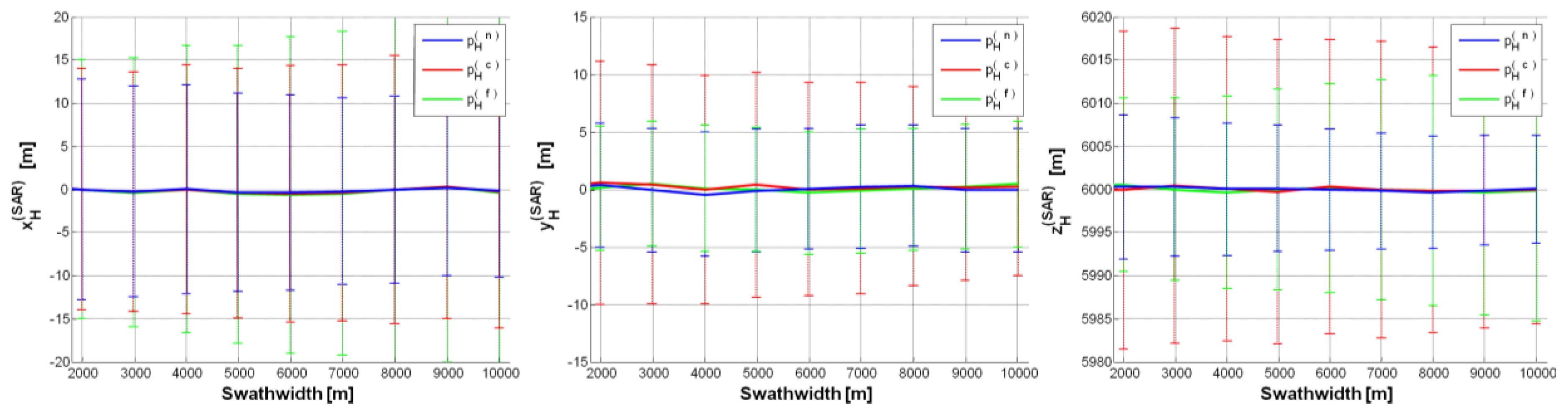
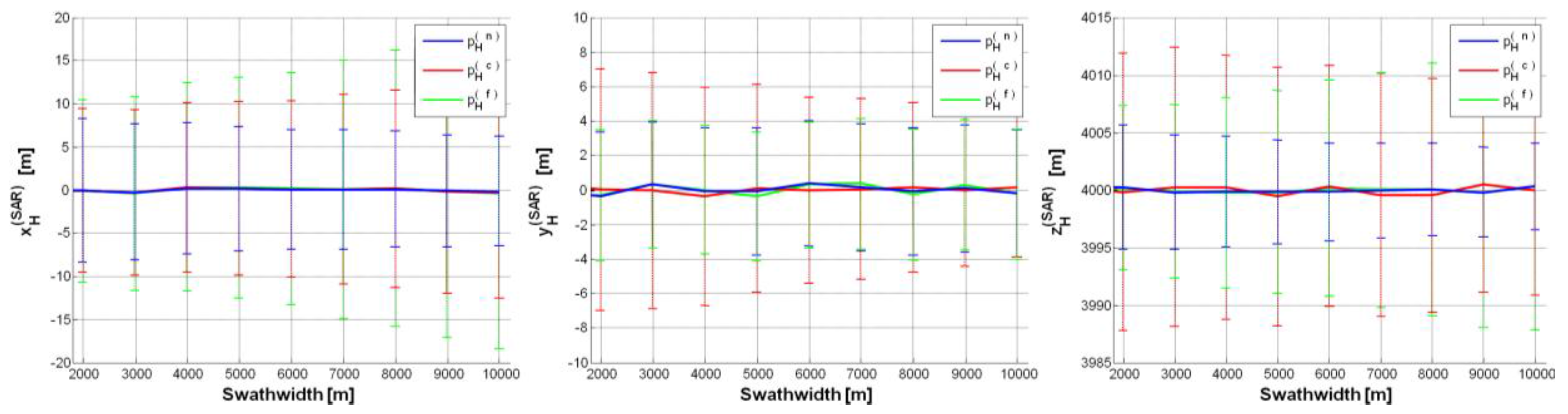
Thus, to reach suitable estimates, we decreased the SAR altitude to
h = 6000 m (case study CS#2 in
Table 2). The results from the “best” configuration are shown in
Figure 5. It can be seen that all the estimated components of
have no bias and their variability is always bounded within ±20 m. Fairly worse results are achieved by exploiting
as landmark, because of the higher uncertainty on the corresponding depression angle
θc. Moreover, the estimates of
based on
are generally better than those based on
, because the impact of IMU inaccuracy is stronger on
θf than on
θn (
θf <
θn).
Figure 4.
SAR position estimates (CS#1 in
Table 2) based on a single GCP (
,
,
):
m,
θ0 = 10°,
, Δ
h = 0.5%, Δ
p = ±2. Error (on each SAR position component) mean value curve as a function of swath-width (
d); error bars show the error standard deviation along the curve.
Figure 4.
SAR position estimates (CS#1 in
Table 2) based on a single GCP (
,
,
):
m,
θ0 = 10°,
, Δ
h = 0.5%, Δ
p = ±2. Error (on each SAR position component) mean value curve as a function of swath-width (
d); error bars show the error standard deviation along the curve.
Figure 5.
SAR position estimates (CS#2 in
Table 2) based on a single GCP (
,
,
):
m,
θ0 = 30°,
, Δ
h = 0.5%, Δ
p = ±2.
Figure 5.
SAR position estimates (CS#2 in
Table 2) based on a single GCP (
,
,
):
m,
θ0 = 30°,
, Δ
h = 0.5%, Δ
p = ±2.
Figure 6.
SAR position estimates (CS#3 in
Table 2) based on a single GCP (
,
,
):
m,
θ0 = 40°,
, Δ
h = 0.5%, Δ
p = ±2.
Figure 6.
SAR position estimates (CS#3 in
Table 2) based on a single GCP (
,
,
):
m,
θ0 = 40°,
, Δ
h = 0.5%, Δ
p = ±2.
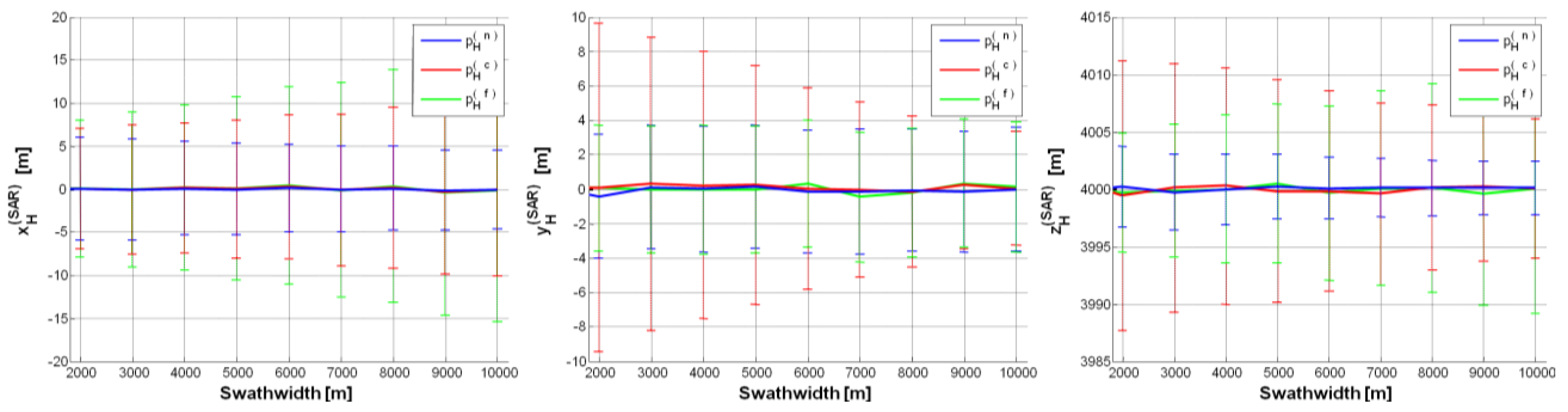
Figure 7.
SAR position estimates (CS#4 in
Table 2) based on a single GCP (
,
,
):
m,
θ0 = 30°,
, Δ
h = 0.5%, Δ
p = ±2.
Figure 7.
SAR position estimates (CS#4 in
Table 2) based on a single GCP (
,
,
):
m,
θ0 = 30°,
, Δ
h = 0.5%, Δ
p = ±2.
Figure 8.
SAR position estimates (CS#5 in
Table 2) based on a single GCP (
,
,
):
m,
θ0 = 40°,
, Δ
h = 0.5%, Δ
p = ±2.
Figure 8.
SAR position estimates (CS#5 in
Table 2) based on a single GCP (
,
,
):
m,
θ0 = 40°,
, Δ
h = 0.5%, Δ
p = ±2.
We also considered a case study (CS#3 in
Table 2) with greater SAR depression angle (
θ0 = 40°), while keeping platform
h as in CS#2.
Figure 6 show CS#3 results, which keep on satisfying the constraint on position accuracy. Note that the accuracy on
is improved compared with CS#2, but it is worse on
, because of the wider Δ
θ0 for
θ0 = 40° than for
θ0 = 30° (
i.e., CS#2) needed to illuminate the same swath-width. For depression angles higher than 40°, the accuracy on the estimates further worsens: such a trend can be also observed by comparing
Figure 5 and
Figure 6.
As a limiting case, we reduced the UAV altitude down to
h = 4000 m (CS#4 in
Table 2).
Figure 7 shows position estimates under the “best” configuration (
θ0 = 30°): the estimated
components show negligible bias and their variability is even lower than in the previous case studies,
i.e., ±15 m. Note that, for swath-width greater than 7000 m, only
exceeds the previous boundary.
We also considered a further case study (CS#5 in
Table 2) with a depression angle
θ0 = 40° greater than in CS#4. All the estimates shown in
Figure 8 are rigorously bounded within ±15 m and SAR position estimates are generally very similar to those achieved in CS#4. Only the inaccuracy on
slightly increases, because of the wider Δ
θ0 for
θ0 = 40° than for
θ0 = 30°. Again, for depression angles higher than 40°, the accuracy on the estimates further worsens.
A UAV altitude lower than 4000 m cannot be taken into account because it would have severe consequences on both SAR system requirements and SAR data processing. In fact, in order to keep constant the values of both
θ0 and swath-width, the lower the altitude, the wider Δ
θ0, thus leading to considerably increasing the required transmitted power. Moreover, a wide Δ
θ0 means large resolution changes across the ground swath [
8], which negatively impact the performance of the ATR algorithm: features that are clearly distinguishable at far range can become nearly invisible at near range.
In conclusion, feasible parameter settings are those relative to CS#2 and CS#4 configurations, which provide estimated UAV coordinates with errors bounded within ±18 m and ±12 m, respectively. In
Table 3, a résumé of the suggested requirements,
i.e., a first trade-off, is listed. Note that the suggested range of SAR swath-width
d (
i.e., few kilometres) allows us to be confident about the presence of the desired landmarks within the illuminated area, even if the SAR system (due to uncertainty on attitude and position) points at the wrong direction. It is worth noting that SAR requirements in
Table 3 can be easily fulfilled by commercial systems, e.g., Pico-SAR radar produced by Selex-ES [
22]; MALE UAV [
10] such as Predator B, Global Hawk and Gray Eagle, which easily carry a Pico-SAR radar; navigation grade class IMU such as LN-100G IMU [
20]; any RALT compliant with the regulation in [
21].
Table 3.
Platform, viewing geometry, navigation sensor requirements and corresponding reference system which allows a feasible SAR position retrieval: first trade-off.
Table 3.
Platform, viewing geometry, navigation sensor requirements and corresponding reference system which allows a feasible SAR position retrieval: first trade-off.
| | First Setting (CS#2) | Second Setting (CS#4) |
|---|
| Aircraft altitude (km) | 6 | 4 |
| Depression angle θ0 (°) | 30 | 30 |
| Swath-width d (km) | few units | few units |
| Elevation beam-width Δθ0 (°) | ≥11.5 | ≥16.6 |
| Image resolution (m) | ~1 |
| SAR band | X |
| SAR polarization | VV |
| Rn (km); R0 (km); Rf (km) | 10.3−9.2; 12; 14.6−18.0 | 6.5−5.7; 8; 10.8−14.7 |
| Maximum detection range Rf (km) | ≥14.6 | ≥10.8 |
| Δh (%) | 0.5 (or fairly worse) | 0.5 (or fairly worse) |
| (°) | 0.05 | 0.05 |
| Estimated UAV based on (bias ± std) (m) | 0 ± 15, 0 ± 11, 0 ± 18 (Figure 5) | 0 ± 12.5, 0 ± 7.5, 0 ± 12 (Figure 7) |
| Reference systems | MALE UAV, e.g.,: Predator B, Global Hawk, Gray Eagle |
| Pico-SAR |
| Any RALT compliant with the regulation in [21] |
| Navigation grade class IMU, e.g.,: LN-100G IMU |
2.4. Landmark DB and Mission Planning
In order to retrieve SAR position, the proposed algorithm has to exploit landmark points. In the previous section, it is assumed that landmark coordinates in the mission DB are ideal,
i.e., without errors. Such an assumption is quite unlikely, and, consequently, we also evaluated the impact of landmark coordinate inaccuracy on the estimated UAV position. According to the previous analysis, preliminary requirements were derived for the landmark DB reference domain, typology, and accuracy. Concerning the reference domain, an inertial system of coordinates (
H) can be adopted, e.g., Earth-centered frame or local map coordinate system. Concerning the landmark typology, planar landmarks (e.g., crossroad, roundabout, railway crossing) are strongly suggested because they are very recurrent in several operating scenarios, can be precisely extracted, and do not introduce any vertical distortion due to elevation with respect to the ground surface [
8]. Small 3D-landmarks can be also exploited but in the limits of the visibility problems due to the shadow areas occurring close to high structures. According to this, a mission planning should avoid scenarios densely populated by buildings, while preferring suburban or rural areas.
Concerning landmark DB accuracy, we exploited the procedure in
Section 2.2 and the most promising two settings in
Section 2.3.
Table 4 presents the platform geo-referencing accuracy derived under two different error settings: a “moderate” DB accuracy with RMSE equal to [3, 3, 3]
t in (m) on landmark coordinates of
, and a “low” DB accuracy with RMSE equal to [3, 3, 10]
t in (m). Results show a limited increase in the final std values with respect to the ideal results in
Section 2.2.
The DB accuracy assumed above is quite reasonable, because the coordinates of interest refer to centroid and corners of small landmarks, and can be derived by exploiting a Geographic Information System (GIS) archive (or similar) [
23]. The mapping standards employed by the United States Geological Survey (USGS) specifies that [
24]: 90% of all measurable horizontal (or vertical) points must be within ±1.01 m at a scale of 1:1200, within ±2.02 m at a scale of 1:2400, and so on. Finally, the errors related to the geo-referencing could be modelled as a rigid translation of a landmark with respect to its ideal position, with RMSE smaller than 10 m.
Table 4.
Platform position retrieval (bias ± standard deviation of each coordinate) as a function of the settings in
Table 1 and Data Base (DB) accuracy on landmark coordinates of
.
Table 4.
Platform position retrieval (bias ± standard deviation of each coordinate) as a function of the settings in Table 1 and Data Base (DB) accuracy on landmark coordinates of .
| Landmark DB Accuracy | CS#2 | CS#4 |
|---|
| “Moderate“ (rmse [3, 3, 3]t in (m)) | 0 ± 14.8 m, 0 ± 10.2 m, 0 ± 17.8 m | 0 ± 12.4 m, 0 ± 05.8 m, 0 ± 12.1 m |
| “Low“ (rmse [3, 3, 10]t in (m)) | 0 ± 14.6 m, 0 ± 10.2 m, 0 ± 20.2 m | 0 ± 12.4 m, 0 ± 05.8 m, 0 ± 15.3 m |


 ,
, 


