The prototype has been implemented in a Java program, and experiments are conducted for evaluating the performance and efficiency of our event coverage detection and event source determination mechanisms. In the following, we introduce the environment settings, present the results of experiments and compare our technique to CARPas the protocol for routing sensory data to SN.
5.2. Experimental Evaluation
Experiments have been conducted for evaluating the performance and efficiency of our event coverage detection and sensory data routing mechanisms. Without loss of generality, the network space is defined as a rectangular region, and SN is located at the center of the ocean surface with the geographical coordinate of (0.5, 1, 0), where the z-coordinate corresponds to the depth of SN (or sensor nodes). The results of our experimental evaluation are presented and discussed in the following.
Table 1.
Experiential parameters settings.
Table 1.
Experiential parameters settings.
| Parameter Name | Value |
|---|
| Simulation network region (km) | 1 × 2 × |
| Number of sensor nodes (including one sink node) | 61 |
| Transmission radius r (km) | |
| Time slots for experiments | 10, 20, 30 |
| EPING or control packet size (B) | 11 |
| EPONG or HELLO control packet size (B) | 7 |
| ACK and getData control packet size (B) | 6 |
| Data packet payload size (B) | 100 |
| Robustness factor for the parent-child relation determination | |
| Smoothing factor for the link quality computation | |
| Power for transmitting a data packet (W) | |
| Power for transmitting a control packet (W) | |
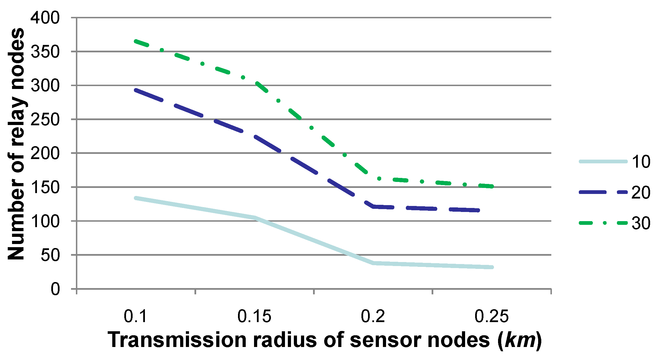
Figure 2.
Comparison of the number of relay nodes when the transmission radius r is set to various values, where 10, 20 and 30 specify the number of time slots for our experiments. This figure shows that the number of relay nodes declines when the transmission radius is set to a relatively large value.
Figure 2 shows the number of relay nodes when the transmission radius
r is set to 0.1, 0.15, 0.2 or 0.25, respectively. The experiments are conducted over 10, 20 or 30 contiguous time slots, and the number of sensor nodes, whose sensory data may deviate from a normal sensing range, is set as 30 at each time slot. Note that “number of relay nodes” in this figure, as well as that in
Figure 3 is the number in total for all relay nodes in these 10, 20 or 30 time slots. Due to the water dynamics, it is assumed that no more than five sensor nodes may drift away during each time slot, and their
x- and
y-coordinates may change no more than 3–5 m, while their
z-coordinate may change no more than 0–3 m.
Figure 2 shows that the number of relay nodes declines to a certain extent when
r is set to a relatively large value, since the transmission region of a sensor node is relatively larger, and hence, more sensor nodes may select the same relay node according to Algorithm 2 for sensory data gathering and routing to
SN. This figure also shows that the number of relay nodes is non-linear with the value of the transmission radius
r, since the transmission region (
i.e.,
) increases much quicker than
r. Consequently, when
r increases, the number of sensor nodes within the transmission region of a certain relay node may increase to a large extent, which results in a decrease in the number of relay nodes. Besides, the number of relay nodes shown in this figure is almost the same when
r is set to 0.2 or 0.25. After examining the deployment of sensor nodes, it is found that, given two candidate relay nodes, the increase for the number of sensor nodes that one candidate node can relay is almost the same as that for another. This means that the determination of relay nodes may not change for sensor nodes, and hence, the number of relay nodes may not change, as well. This fact indicates that the density of deviated sensor nodes (a more detailed discussion is presented in
Figure 4), which is determined by the number of deviated sensor nodes and the communication radius, is the key factor for determining the number of relay nodes.
Figure 3 shows the number of relay nodes when the number of sensor nodes (denoted
), whose sensory data deviate from a normal sensing range, is set to 20, 30, 40 or 50, respectively. The communication radius
r is set to 0.1, 0.15 or 0.2, respectively. Note that the experiments for
r as 0.25 are not discussed, since
r as 0.25 is relatively too large with respect to the network region, and the results of the experiments may not be convincing. This figure shows that the number of relay nodes increases to an extent when
is set to a relatively large value. Note that when
is quite large (e.g., 40 or 50), the increasing of the number of relay nodes is relatively small. This is due to the fact that when
is relatively large, sensor nodes, whose sensory data deviate from a normal sensory range, are densely distributed in the network. Consequently, a relay node may have to relay sensory data for a relatively larger number of deviated sensor nodes, but relay nodes may not need to be newly added. In this setting, the workload of relay nodes should be increased, which should cause the increase of energy consumption in total. However, the number of relay nodes may not increase to an extent.
Figure 3.
Comparison of the number of relay nodes when the number of sensor nodes (denoted ), whose sensory data deviate from a normal sensing range, is set to various values. This figure shows that the number of relay nodes increases significantly when is set to a relatively large value.
Figure 3.
Comparison of the number of relay nodes when the number of sensor nodes (denoted ), whose sensory data deviate from a normal sensing range, is set to various values. This figure shows that the number of relay nodes increases significantly when is set to a relatively large value.
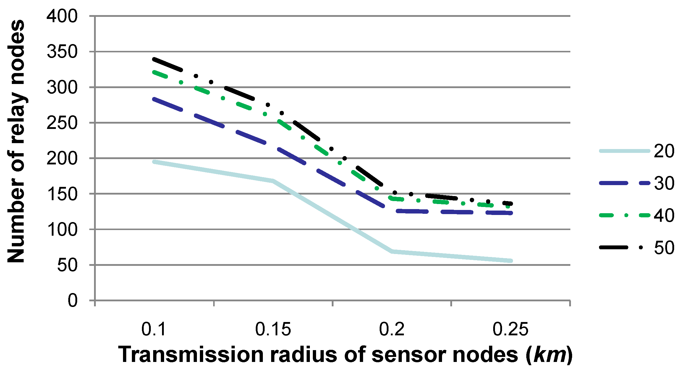
Figure 4.
Comparison of the number of relay nodes when the transmission radius r is set to various values and the number of deviated sensor nodes is set to 20, 30, 40 or 50, respectively. This figure shows that the number of relay nodes is mostly impacted by the density of deviated sensor nodes, which is determined by r and the number of deviated sensor nodes in the network region.
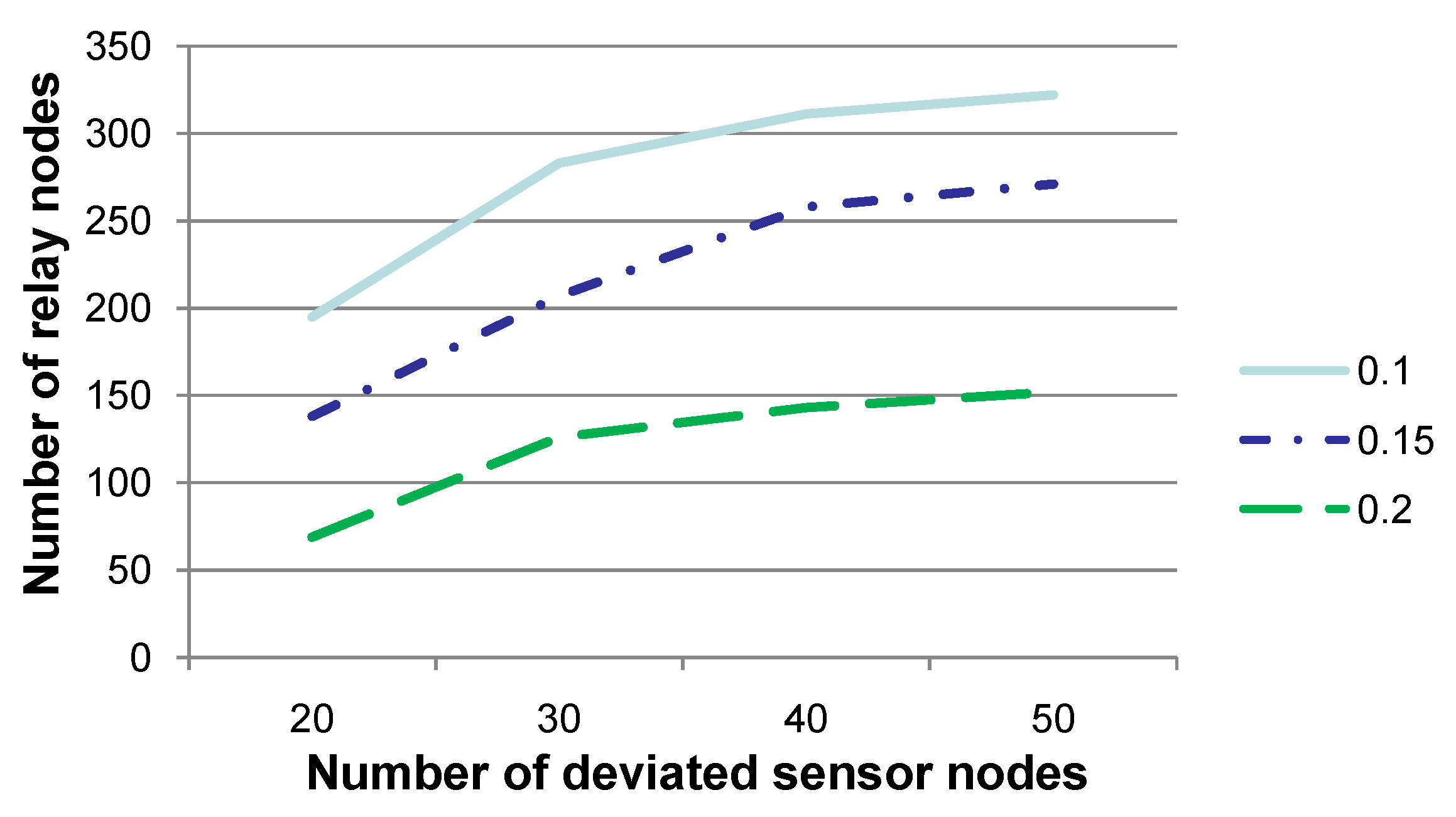
Figure 4 shows the number of relay nodes when the transmission radius
r is set to 0.1, 0.15, 0.2 or 0.25, respectively, while the number of deviated sensor nodes is set to 20, 30, 40 or 50, respectively. The other parameters are set to the same values as those in
Figure 3.
Figure 4 shows that the increase of the number of relay nodes is non-linear with that for the number of deviated sensor nodes. In fact, the density of deviated sensor nodes in the network region is the key factor for determining the number of relay nodes, where the density can be represented as the average number of deviated sensor nodes contained in a sphere whose radius is
r. Generally, when deviated sensor nodes are relatively sparely deployed in the network region (for instance, the number of deviated sensor nodes is 20 or 30), newly-added deviated sensor nodes
may require newly-added relay nodes for sensory data gathering and routing to
SN, since existing relay nodes may hardly cover
. On the other hand, when the number of deviated sensor nodes is large enough (for instance, 40 or 50), relay nodes may have covered the whole network region already. Consequently, newly-added deviated sensor nodes can be relayed by existing relay nodes, although their workload is much heavier than before. As argued in
Figure 2, the number of relay nodes is mostly decided by the density, rather than the number of deviated sensor nodes.
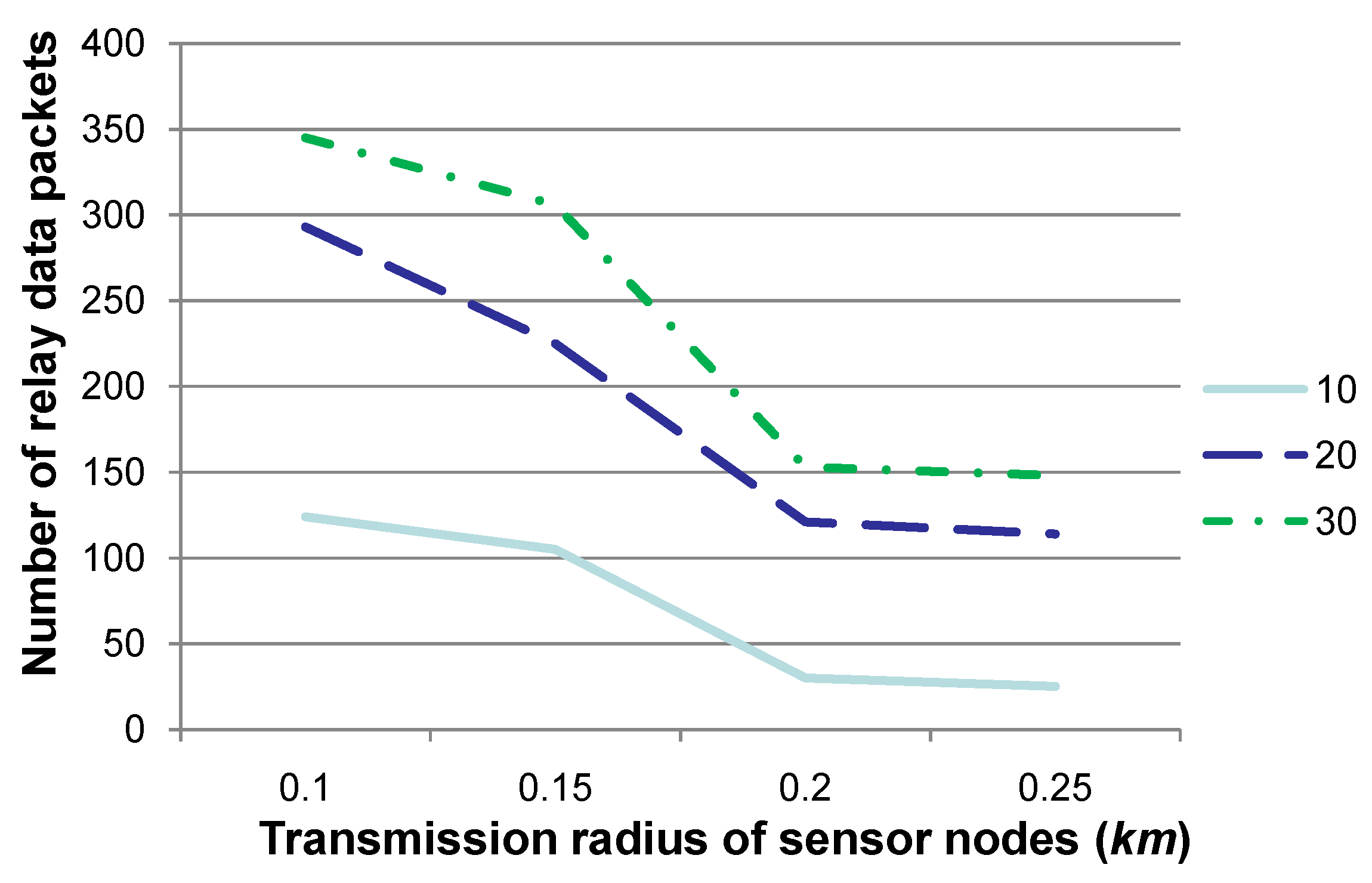
Figure 5.
Comparison of the number of relay data packets when the transmission radius r is set to various values. This figure shows that the number of relay data packets declines when the transmission radius is set to a relatively large value.
Figure 5.
Comparison of the number of relay data packets when the transmission radius r is set to various values. This figure shows that the number of relay data packets declines when the transmission radius is set to a relatively large value.
Figure 5 shows the number of relay data packets when the transmission radius
r is set to 0.1, 0.15, 0.2 or 0.25, respectively. Similar to “number of relay nodes” in
Figure 2, “number of relay data packets” in this figure specifies the number in total for all relay nodes in these 10, 20 or 30 time slots. The other parameters are set to the same values as those in
Figure 2.
Figure 5 shows that the number of relay data packets decreases when
r is set to a relatively large value. However, when
r is large enough (e.g., 0.2 or 0.25), the number of relay data packets is almost the same. Similar to the explanation in
Figure 2, the relation for sensor nodes and the corresponding relay nodes may not change somehow when
r is large. This means that the number of relay data packets may not change, as well, although hop counts may be decreased when routing relay data packets to
SN, which may cause the decrease of energy consumption.
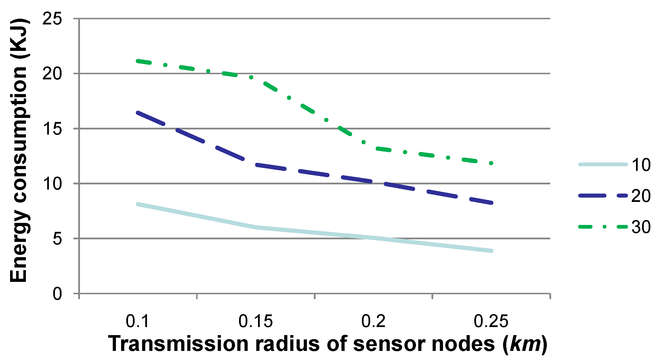
Figure 6 shows the energy consumption when the transmission radius
r is set to 0.1, 0.15, 0.2 or 0.25, respectively. The other parameters are the same as those in
Figure 2. Similar to “number of relay nodes” in
Figure 2, “energy consumption (KJ)” in
Figure 6 specifies the energy consumed in total for all relay nodes in these 10, 20 or 30 time slots.
Figure 6 shows that the energy consumption decreases when
r is set to a relatively large value. This is due to the fact that the number of relay data packets decreases when
r increases. As indicated by the values in
Table 1, the smaller the number of data (or control) packets is to be transmitted, the less the energy is to be consumed. As presented by
Figure 5, when
r is large enough, the number of relay data packets is almost steady. Therefore, the energy consumption may not decrease to an extent. It is worth mentioning that when
r is large, there may exist relay nodes that may relay sensory data for a single sensor node. This may induce an imbalance of energy consumption between relay sensor nodes and may be harmful to the network lifetime. Consequently, a tradeoff should be considered when setting a value for
r in real applications.
Figure 6.
Comparison of energy consumption when the transmission radius r is set to various values. Generally, the larger the value of r is, the less the energy consumption is for sensory data gathering and routing to SN.
Figure 6.
Comparison of energy consumption when the transmission radius r is set to various values. Generally, the larger the value of r is, the less the energy consumption is for sensory data gathering and routing to SN.
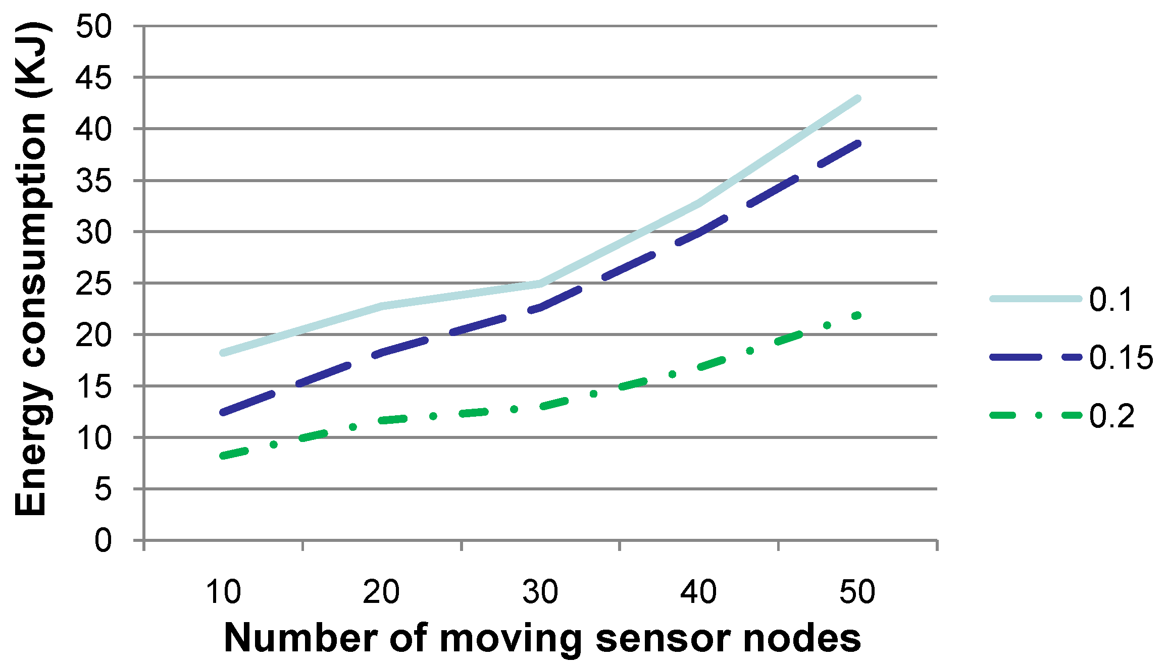
Figure 7 shows the energy consumption when the number of sensor nodes, which drift with the water dynamics and change their coordinates, is set to 10, 20, 30, 40 or 50, respectively, where the
x- and
y-coordinates of these sensor nodes change no more than 3–5 m and their
z-coordinate changes no more than 0–3 m, per time slot. The energy consumption is the amount in total for the experiments conducted for 20 time slots. The other parameters are set to the same values as those in
Figure 2. As presented by Algorithm 2, the larger the number of sensor nodes whose coordinates change is, the larger the number of relay nodes that have to be re-selected and the larger the number of
-EPONG control packets to be transmitted. Therefore, more energy is to be consumed during the relay nodere-selection phase, as shown in
Figure 7. This figure indicates that our technique is more energy efficient when the network topology is relatively steady.
Figure 7.
Comparison of energy consumption when the number of sensor nodes, which drift with the water dynamics and change their coordinates, is set to various values. This figure shows that the larger the number of sensor nodes changing their coordinates, the more energy is to be consumed.
Figure 7.
Comparison of energy consumption when the number of sensor nodes, which drift with the water dynamics and change their coordinates, is set to various values. This figure shows that the larger the number of sensor nodes changing their coordinates, the more energy is to be consumed.
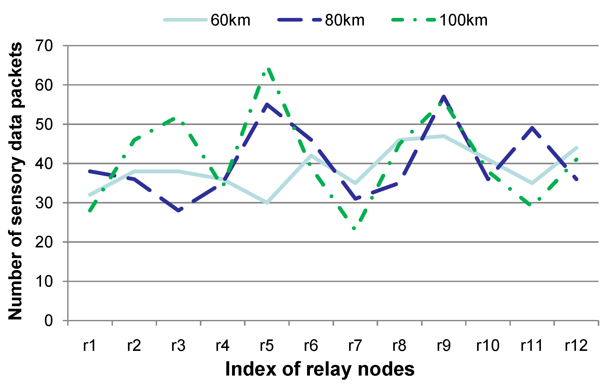
Figure 8 shows the number of sensory data packets that a certain relay node delivers, when sensor nodes are deployed in the network space under various skewness distributions. Intuitively, two sensor nodes (denoted
and
) can have a link, when the geographical distance
between
and
is shorter than the communication radius
r. Given the set
}, the variance is adopted to represent the skewness degree of the sensor node distribution. Generally, when the variance is smaller, which means that the geographical distances between sensor nodes are more similar, sensor nodes are distributed more evenly in the network region. In our experiments, three kinds of sensor node distributions have been generated and their variances are 60 km, 80 km or 100 km, respectively. The experiments are conducted for 20 contiguous time slots, and the other parameters are set to the same values as those in
Figure 5. Twelve relay nodes are selected for studying the number of sensory data packets to be forwarded, and these 12 relay nodes are represented as
, ⋯,
in
Figure 8. Note that these 12 relay nodes include those having the largest, and the smallest, number of sensory data packets.
Figure 8 shows that the distribution of the number of sensory data packets is relatively even when the variance is relatively smaller (
i.e., the variance is 60 km), although the number of sensory data packets for certain relay nodes may be smaller when the variance is relatively larger (
, for instance). This is due to the fact that sensor nodes are distributed in a more skewed fashion when the variance is relatively larger. Therefore, the workload of relay nodes is more uneven, which is reflected by the number of sensory data packets in
Figure 8. Note that relay nodes with a larger number of sensory data packets should consume more energy and may die earlier than the others. This is harmful to the network lifetime. Therefore, a relatively even distribution of sensor nodes is beneficial for balancing the energy consumption of relay nodes.
Figure 8.
Comparison of the number of sensory data packets when sensor nodes are deployed in diverse skewness distributions in the network region. This figure shows that different sensor node deployment strategies may have a relatively large impact on the number of sensory data packets to be forwarded by certain relay nodes.
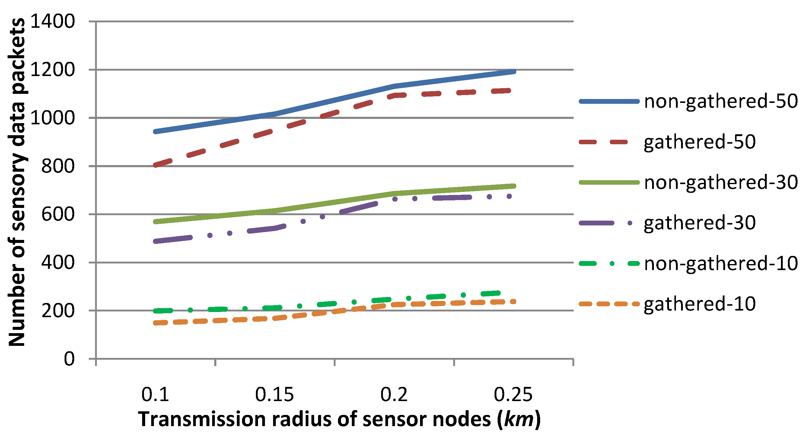
Figure 9 shows the number of sensory data packets, when sensory data are gathered by relay nodes, or are not gathered, and will be routed by individual sensor nodes through the routing tree independently. The transmission radius
r is set to 0.1, 0.15, 0.2 or 0.25, respectively. The experiments are conducted for 20 contiguous time slots. There are 10, 30 or 50 sensor nodes in each time slot whose sensory data deviate from a normal sensing range, which are specified in
Figure 9 and in
Figure 10, as gathered, 10/30/50, and non-gathered, 10/30/50, respectively. The other parameters are set to the same values as those in
Figure 5.
Figure 9 shows that the number of sensory data packets is smaller for the gathered cases, when
r is relatively smaller. This is due to the fact that sensory data of several sensor nodes can be gathered as a single data packet, which should be routed to
SN with relatively large hops through the routing tree. Hence, the number of sensory data packets can be reduced to a large extent, in comparison with that of the non-gathered cases. This experiment shows the advantage of our sensory data gathering strategy than the traditional non-gathered one on reducing the number of sensory data packets.
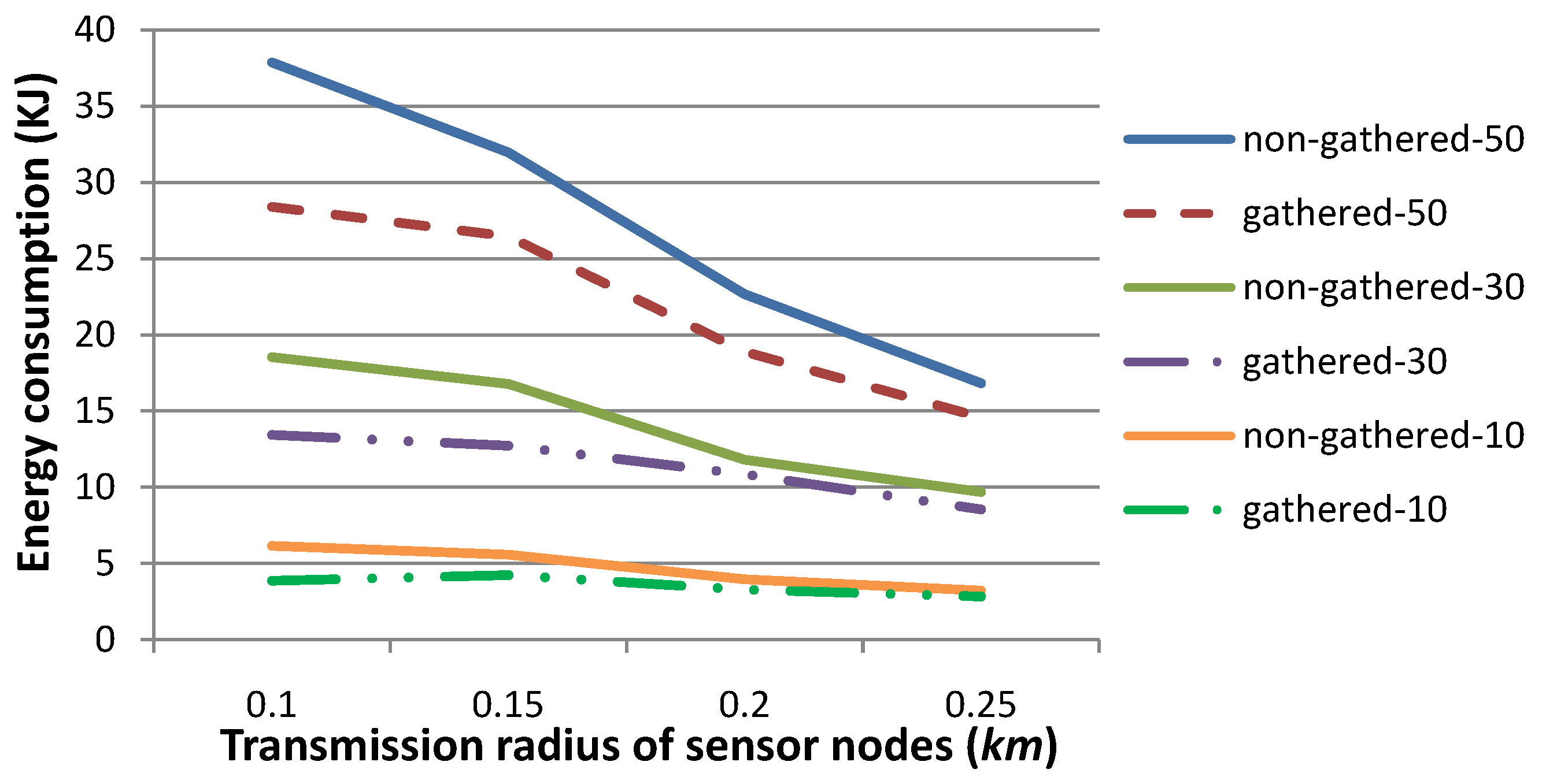
Figure 10 shows the energy consumption for the gathered or non-gathered scenarios. As presented in
Figure 9, sensory data packets are much fewer for gathered cases when the transmission radius
r is set to a relatively smaller value, and hence, energy consumption is also quite less in this situation, although sensory data packets should be larger in size for the gathered strategy than for the non-gathered strategy. Consequently, our gathered strategy is more energy efficient, especially when
r is set to a relatively small value.
Figure 9.
Comparison of the number of sensory data packets when the transmission radius r is set to various values, for the strategies that sensory data are gathered, or not gathered, by relay nodes. This figure shows that our gathered strategy requires a smaller number of sensory data packets than the number that non-gathered strategy requires, especially when r is set to a relatively small value.
Figure 10.
Comparison of the energy consumption when the transmission radius r is set to various values, for the strategies that sensory data are gathered, or not gathered, by relay nodes. This figure shows that the energy consumption for our gathered strategy is smaller than that for the traditional non-gathered strategy, especially when r is relatively small.
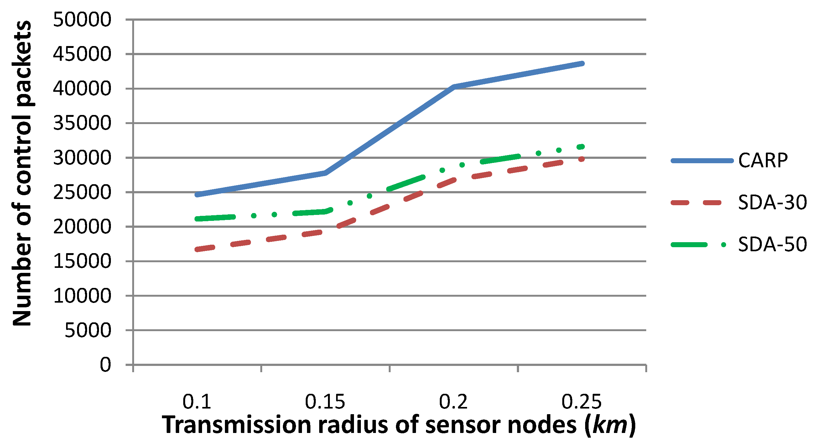
5.3. Comparison with CARP for the Number of Control Packets and Energy Consumption
This section presents the result of our experiments for our sensory data gathering technique (denoted SDA in the following) with respect to CARP [
27], where CARP serves as the protocol for routing sensory data to
SN. As mentioned before, the routing strategy adopted in our technique is developed through improving the mechanism of CARP.
Figure 11 shows the number of control packets generated by (i) our technique and (ii) CARP as the routing protocol, when the transmission radius is set to 0.1, 0.15, 0.2 or 0.25, respectively. The number of sensor nodes, which drift with the water dynamics and change their coordinates, is set to 30 or 50, respectively, where the
x- and
y-coordinates of these sensor nodes change no more than 3–5 m and their
z-coordinate changes no more than 0–3 m, per time slot. There are 30 sensor nodes at each time slot whose sensory data deviate from a normal sensing range. The other parameters are set to the same values as those in
Figure 5.
Figure 11 shows that the number of control packets for CARP is the same when the number of moving sensor nodes varies, since CARP reselects relay nodes whenever sensory data are required to be routed to
SN, and hence, the number of control packets is not impacted by the number of moving sensor nodes. On the other hand, the number of control packets generated by our technique is much smaller than that by CARP, when the number of sensor nodes, which drift with the water dynamics and change their coordinates, is relatively smaller. This is due to the fact that when the network topology is relatively steady, the number of parent nodes, which are determined in previous time slot(s) and can be reused for routing sensory data to
SN in the forthcoming time slots, are relatively larger in number. Therefore, the number of
-EPONG control packets is smaller. Besides, when the communication radius
r is relatively large, the parent-child relation for a larger number of sensor nodes can be maintained, although their coordinates have been changed. This is reflected by
Figure 11: the difference in the number of control packets is smaller for
r = 0.25 than that for
r = 0.1. Generally, a smaller number of control packets is generated by our technique than by CARP, especially when the network topology is relatively steady.
Figure 11.
Comparison of the number of control packets for our technique (SDA) with respect to CARPas the routing protocol, when the transmission radius r is set to various values, and the number of sensor nodes, which drift with the water dynamics and change their coordinates, is set to various values. This figure shows that the number of control packets generated by our technique is much smaller than that of CARP, especially when the network topology is relatively steady.
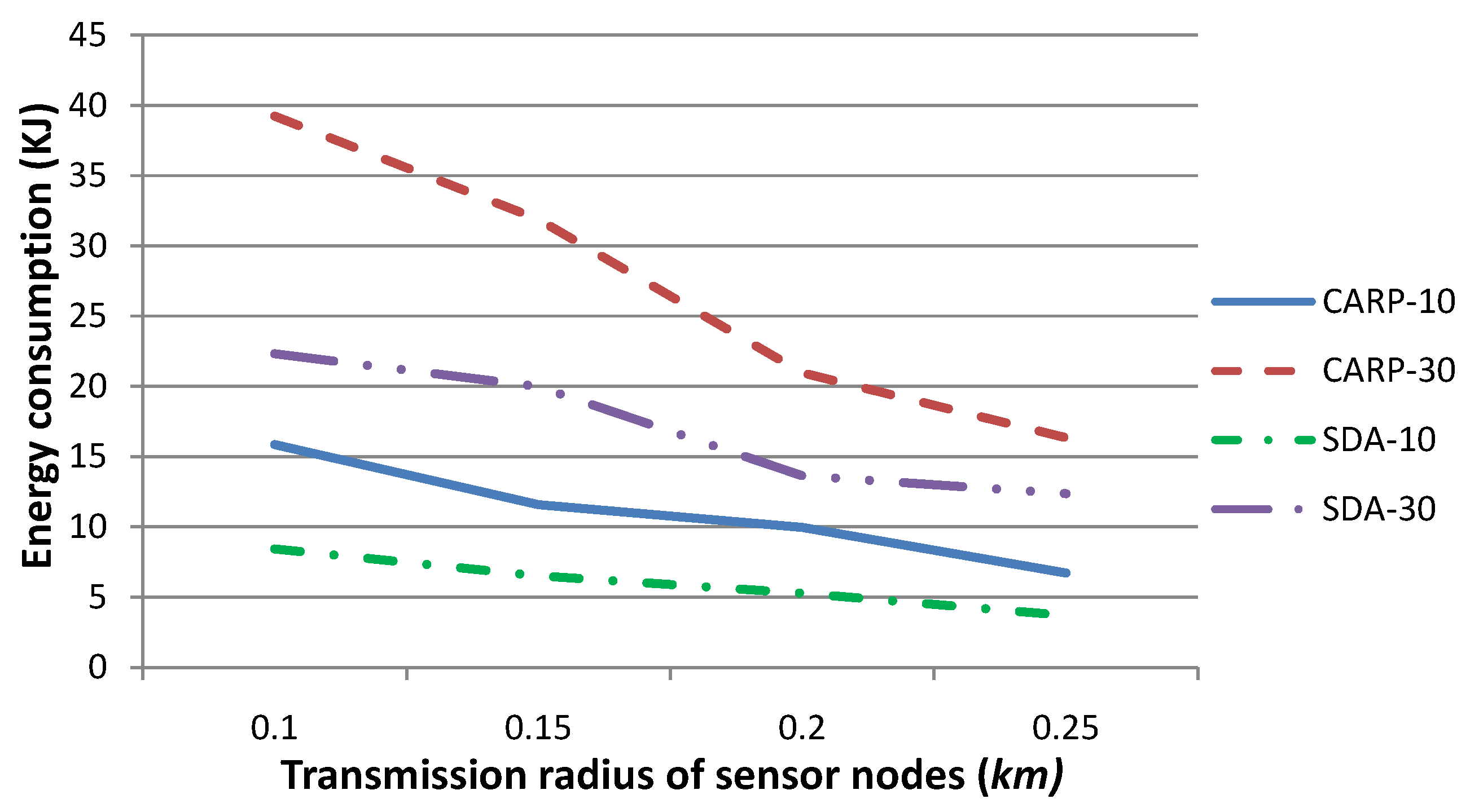
Figure 12 shows the energy consumption for (i) our technique and (ii) CARP as the routing protocol. The transmission radius
r is set to 0.1, 0.15, 0.2 or 0.25, respectively. The experiments are conducted for 10 and 30 contiguous time slots. There are 30 sensor nodes at each time slot whose sensory data deviate from a normal sensing range. The other parameters are set to the same values as those in
Figure 5.
Figure 12 shows that the energy consumption of our sensory data aggregation strategy is less than that of CARP. This is due to the fact that sensory data, whose value has been varied significantly, are gathered and routed to
SN. This means that the partial, rather than the whole of, sensory data should be routed to
SN in a certain time slot. However in CARP, all sensory data should be routed to
SN, and each data packet should be routed independently. Therefore, more energy is to be consumed for data gathering and routing.
Figure 12 also shows that the difference of energy consumption becomes smaller when the transmission radius is set to a relatively large value, since a smaller number of hops are required when routing data packets to
SN. Besides, our technique requires the maintenance of a routing tree, which induces some energy consumption. Generally, our technique is more energy efficient, especially when the transmission radius is a relatively small value.
Figure 12.
Comparison of energy consumption for our technique (SDA) with respect to CARP as the routing protocol, when the number of time slots is set to 10 and 30, respectively. This figure shows that the energy consumption for our technique is less than that of CARP, especially when the communication radius r is set to a relatively small value.
Figure 13.
Comparison of energy consumption for our technique (SDA) with respect to CARP as the routing protocol, when the transmission radius r is set to 0.1 and 0.15, respectively, and the number of sensor nodes, which drift with the water dynamics and change their coordinates, is set to various values. This figure shows that the energy consumption for our gathered strategy is much smaller than that of CARP, especially when the number of moving sensor nodes is relatively small.
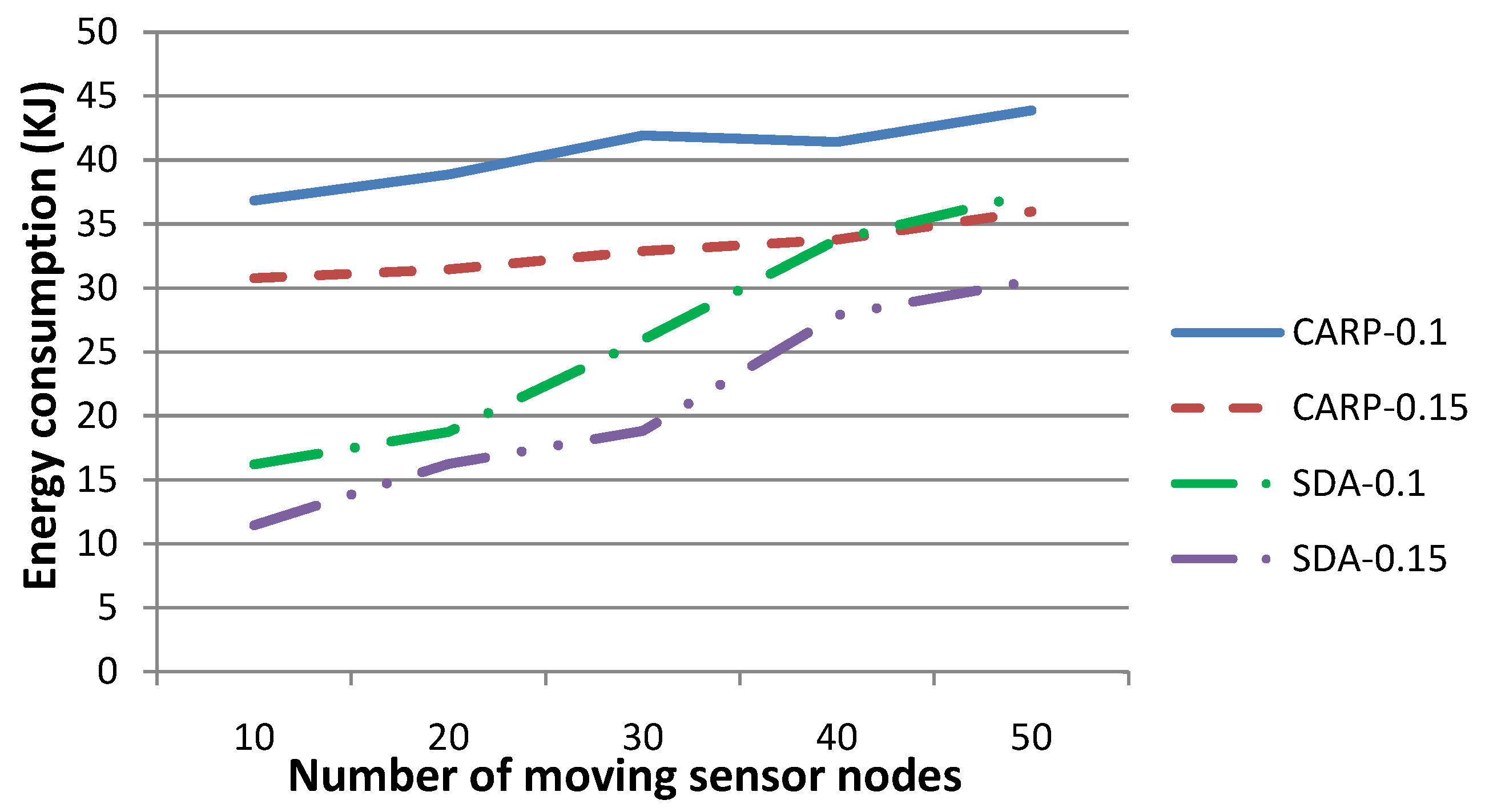
Figure 13 shows the energy consumption for (i) our technique and (ii) CARP as the routing protocol. The transmission radius
r is set to 0.1 and 0.15, respectively. The number of sensor nodes, which drift with the water dynamics and change their coordinates, is set to 10, 20, 30, 40 or 50, respectively, where the
x- and
y-coordinates of these sensor nodes change no more than 3–5 m and their
z-coordinate changes no more than 0–3 m, per time slot. The other parameters are the same as those in
Figure 12.
Figure 13 shows that our technique requires consuming more energy when the number of moving sensor nodes increases, while that for CARP is relatively steady (although large relatively). In fact, our technique may require one to re-select the parent nodes for sensory data gathering and routing to
SN, while it can hardly reuse the parents determined in previous time slot(s), when a larger number of sensor nodes changes their coordinates frequently. Generally, the larger the number of parent nodes is to be reselected, the larger the number of
-EPONG control packets to be transmitted and the more the energy is to be consumed during the sensory data routing procedure.
Figure 13 shows that the energy consumption increases quickly along the increase of the number of moving sensor nodes. On the other hand, CARP requires one to select the parent nodes whenever a data packet is to be routed. This strategy suggests that the number of moving sensor nodes may not impact the energy consumption to an extent. Consequently, our technique is impacted by the number of moving sensor nodes and is more energy efficient, especially when the network topology is relatively steady.


