1. Introduction
With the improvement of road traffic and the development of vehicle technology, automobiles are moving faster and faster. There is a gradual increase in the role of high-speed instability as a factor in all kinds of traffic accidents. Audi company statistics indicate that with traffic accidents involving vehicles at speeds of 80 km/h to 100 km/h, there was a loss of stability in 40% of the cases [
1]. When the speed exceeds 160 km/h, almost all accidents involve a vehicle that is unstable. Related studies also indicate that in serious traffic accidents caused by the loss of stability control, 82% of vehicles continue to travel for 40 m after loss of control. A Toyota Corporation study also points out that vehicle sideslip motion is involved in almost all accidents caused by loss of control [
2]. Therefore, stability control for vehicles is proposed. Vehicle handling stability is improved by controlling vehicle yaw motion.
Yaw rate and vehicle sideslip angle are the significant parameters [
3] of a vehicle control stability. Usually, the vehicle sideslip angles [
4] are defined as the angles among vehicle velocity direction and the vehicle body’s longitudinal axis. The accurate measurement for the real yaw rate and actual vehicle sideslip angles is the largest problem in vehicles stability control improvement [
5]. A gyro can measures the yaw rate, but there is no desirable facilities which can gauge the vehicle sideslip angle directly, so estimation approaches are used. These approaches are merged with use of the lateral acceleration sensor and yaw rate gyro normally. These sensors, however, contain noise and a bias usually. Besides, lateral gyro sensors cannot present safe description for vehicle acceleration force component [
6]. These sensors’ errors will be cumulated and lead to divergence while the integral is employed, influencing the vehicle stability control system’s performance. The vehicle sideslip angle, however, is directly measurable by means of the utilization in GPS/INS [
7]. DGPS (Differential GPS) can achieve millimeter-level precision since it is appended to a differential rectification signal to amend data processing.
There is a solid complementary [
8] between INS and GPS. GPS possesses a number of disadvantages. For instance, a receiver antenna may drop location data owning to signal disruption or be obstructed for the moment [
9]. INS can supply velocity information, azimuth information and position data beyond an outside reference source but the INS has cumulated bias. It cannot provide accuracy position data for long working hours due to gyro drifting flaw. INS bias is primarily irregular drifting flaws that cannot be reimbursed. On the other hand, GPS advantages include great positioning correctness and no accumulation errors. The combination of two types of system can recompense each one and play to their respective advantages. Although GPS testing is stabilizing, the update rate (1~10 Hz) is comparatively minor. GPS/INS Integration navigating system is a sort of composite system having uncommon superiority in bandwidth. Using the Kalman filter algorithm to fuse GPS/INS data is a common method [
10].
In a data fusion method of multi sensors, in order to estimate the state parameters correctly, each sensor should be synchronized to transmit data [
11]. In the actual global positioning system and inertial navigation system sensors, however, data sent to the Kalman filter are frequently not synchronized. If data from the two system sensors is not synchronized, a flaw will be yielded, decreasing the multi sensors system measuring accuracy [
12]. Therefore, real-time data synchronization is of practical significance for the global positioning system and inertial navigation system sensors. Both INS and GPS have their own clock frequency. Due to the differences in the character of frequency and temperature stability for GPS/INS, there are a number of changes after GPS/INS long operating hours, even though INS and GPS begin at the same time. Additionally, INS and GPS have a distinct data update rate normally (for example, the update rate of INS is 100 Hz or more and the data update rate of GPS receiver is 1~20 Hz) [
13]. If INS and GPS data processing time is not synchronized, time difference will happen in Kalman filter.
GPS/INS is the trend to measure vehicle movement stability in modern automobile technology [
14]. At present, GPS measurement has a low refresh data rate, and sometimes there are obstacles that prevent vehicles from accepting GPS information. Therefore, GPS and inertial sensor combination application is needed. Nowadays there are Kalman federated filtering algorithm, D-S evidence theory, neural network, adaptive H filtering and fuzzy logic for data fusion [
15]. However, each algorithm has limitations. Therefore, more convenient and high precision data fusion algorithm is a very meaningful problem. In addition, adaptive method, error compensation technology, statistical characteristic and noise filtering in data fusion are subjects for future research.
2. Related Work
In general, the stability of vehicles is tested using Global Positioning System. In addition, GPS can supply real time vehicle sideslip angle information to vehicles stability control system as a sensor. Although methods for vehicle stability controlling have been implemented for more than a decade, the GPS/INS integration research in vehicles stability measurement stays long way. There are a few similar reports in this area.
In driving conditions, one of the key vehicle stability controls is the accurate measurement of automobile state parameters. This is also the premise and foundation for the system to control the vehicle’s stability [
16]. However, some important vehicle state parameters either cannot be measured through the sensor, or the measuring cost is too high. For instance, an extremely significant stability parameter for vehicle control is sideslip angles, which are the angles between direction of vehicle speed’s longitudinal axis and the direction of the vehicle body. It directly influences the vehicle yaw moment affecting the automobile’s stability. However, unfortunately there is still no common sensor that can measure the tire sideslip angle and the vehicle sideslip angle directly [
17]. The incomplete information on vehicle stability control has caused great difficulties for the implementation and promotion of the vehicle active safety control system, which requires estimating parameters such as the main adhesion coefficient of the road, the sideslip angle, and speed. Vehicle sideslip angle estimation algorithms are a common integral method, such as the Kalman filtering method, fuzzy observer, Luenberger observer, sliding mode observer and nonlinear observer. Cho proposed a method which can estimate the vehicle sideslip angle based on the extended Kalman filter [
18]. The vehicle speed estimation method is a maximum wheel speed method, a slope method, and a comprehensive method. Solmaz proposed a method of estimation based on rolling horizon vehicle speed. Estimation of road adhesion coefficient mainly has the direct detection method based on sensor and method of vehicle dynamics parameters [
19]. Jun proposed a road friction coefficient estimation method based on an extended Kalman-filter algorithm [
20]. Yang Fuguang proposed real-time road adhesion coefficient estimation method based on extended state observer [
21]. These algorithms are based on vehicle dynamic models. Some models are founded without considering some affects such as lateral slip forces. Those methods would product limitation since the lateral slip forces is relative small sometimes during normal driving condition. In addition, the accelerometers, which were used in those approaches, would drift over time due to sensors bias, so more noise would be present in the measurement.
In vehicle active safety, Deng-Yuan Huang proposed a feature-based vehicle flow analysis approach and measurement system for real-time traffic surveillance system [
22] and Jeng-Shyang Pan proposed a vision optical flow based vehicle forward collision warning system for intelligent vehicle highway applications [
23]. The researchers had a wide scope in vehicle active safety research.
Since the beginning of the 21st Century, Chinese researchers have been conducting research on the measuring stability of state parameters of automobile. These researchers have already made some achievements. Yu Ming
et al in Southeast University developed automobile road five-wheel RTK testers, based on GPS carrier phase RTK technology [
24]. The five-wheel tester can precisely measure vehicle motion parameters and evaluate the vehicle movement performance test based on dynamic measurement. However, the five-wheel tester is a very professional instrument and its cost is very high. Xin Guan and his student in Jilin University have done exploratory studies in GPS/INS integrated navigation algorithm for measuring vehicle state information. The method can precisely measure vehicle state parameters, but the GPS and INS instrument that they used is very expensive.
The research on integration navigation's data fusion has been carried out for ages. Before Kalman filtering, the Lagrange interpolation approach was used to data fusion usually [
9]. The Lagrange interpolation is a classic mathematic approach and an elementary method. However, Lagrange interpolation is a linear interpolation. That is, for a nonlinear system the linear interpolation method is not suitable to interpolate data. The errors of interpolation are not minor. The large errors of interpolation are Lagrange interpolation’s main defect. The final curve of interpolation is also rough [
25].
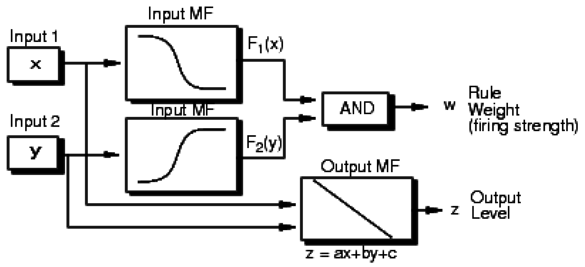
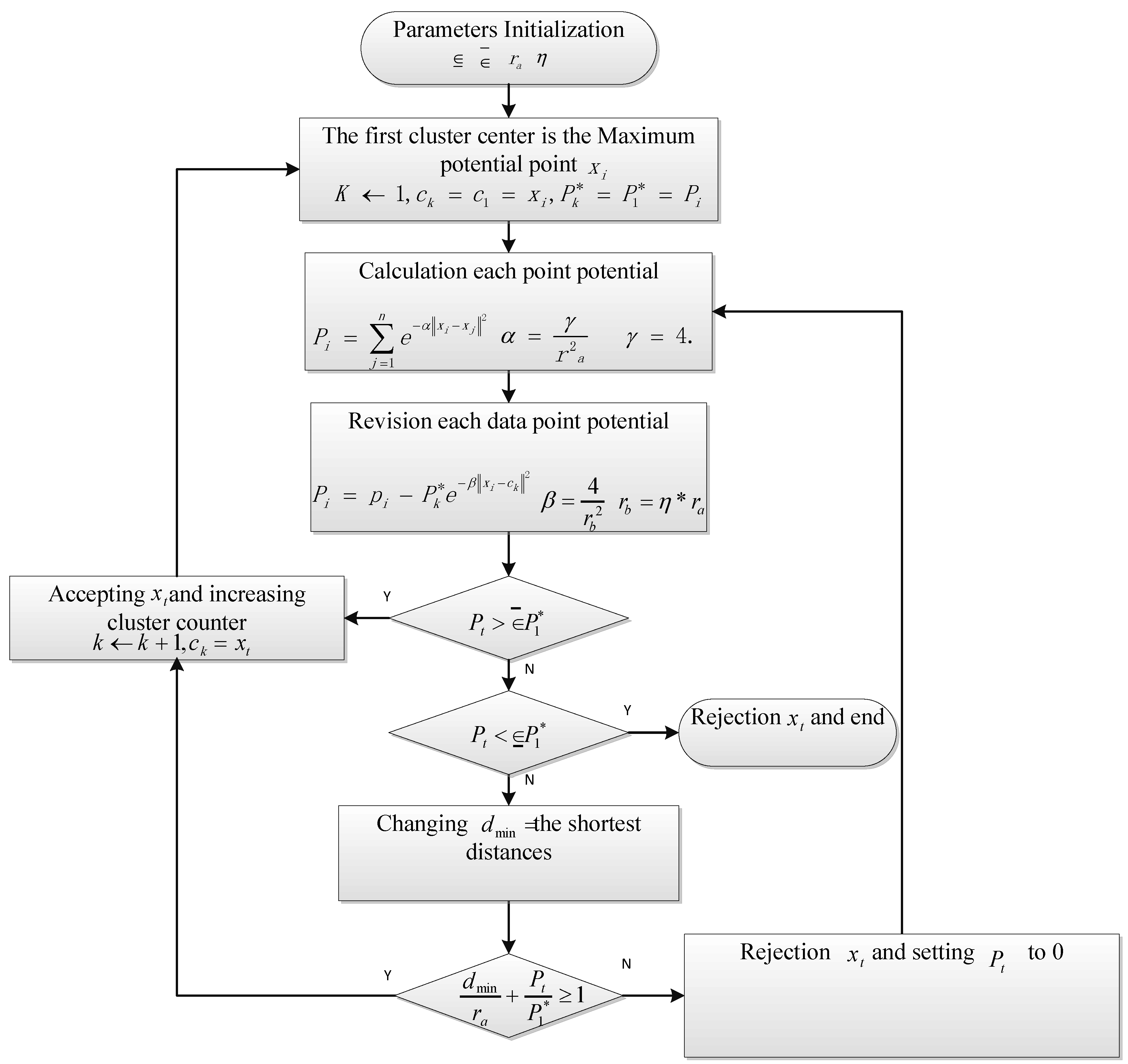
Though the Lagrange interpolation approach can obtain rough values in multi-sensors data fusion system, the method is hard to apply in the general example. This work’s major contribution is to obtain a novel, realistic, and generic method to find out optimum in data fusion. With the fuzzy clustering method’s aid, this work proposed a generic method which optimizes interpolation errors intelligently [
26].
GPS is used for vehicle stability performance testing. It can measure real-time vehicle stability parameters such as running track, distance, azimuth, sideslip angle, speed and acceleration. Differential GPS technology cannot only achieve the online dynamic testing function of motion-state parameters, it also brings the dynamic positioning precision to within the centimeter level. GPS and inertial navigation system is combined in the vehicle motion measurement system of British Oxford Technical Solutions company, in which speed precision is up to 0.05 km/h, and sideslip angle accuracy is up to 0.15°. Zhang Sumin used the inertia navigation system and GPS to estimate vehicle speed, vehicle sideslip angle, yaw rate and other status information [
27]. Kirstin L. Rock at Stanford University used GPS and auto optics test system to measure for comparative experiments, and verify the effectiveness of the GPS/INS to measure the vehicle sideslip angle and speed [
28]. Zhibin Shuai described the electrical vehicles’ lateral motion control related to on-board network-induced time delays. Co-simulations with CarSim and Simulink demonstrate the proposed controller’s effectiveness [
29]. Tommaso Goggia introduces an essential sliding mode formulation for the torque-vectoring control of a fully electric vehicle. A meaning enhancement of controlled vehicle performance is shown during all maneuvers [
30].
Binh Minh Nguyen concentrated on a novel electronic vehicles stability control system that was based on sideslip angles estimation by using Kalman filter. Through dealing with the combination of external disturbances and model flaws as prolonged states in a Kalman filter algorithm, precise sideslip angle estimation was accomplished [
31]. Jin-Oh Hahn built a novel tire road friction coefficients approximation algorithm that is based on measurements relevant to lateral dynamics of the developed vehicle. The advantage is that it does not need big longitudinal slip to provide responsible friction estimations [
32]. Auburn Bevly gauged three important vehicle stability parameters like tire sideslip angle, tire-slip ratio, and sideslip angle that was based on the GPS velocity gauging approach [
33]. They adopted the integration between GPS velocity sensors and inertial testing unit with a low update rate gyro. A new update algorithm for enhancing Kalman filtering was proposed for the tire lateral stiffness. A precise estimate of vehicle state values was provided. However, the robustness of the approach is not verified with some lateral disturbance. The vehicle multi-sensor research center of Calgary University have a research on suppressing bias and enhancing precision in details [
18]. They presented a measurement method that can decrease the accumulated errors while GPS signals are lost. Ryu at Stanford University put an approach forward to estimate vehicle stability's key parameters, which used a combination of INS and GPS sensors [
34]. The approach could enhance estimation’s precision for vehicle state parameters in consideration the influence of roll, pitch and sensors bias. Although this method can measure the key vehicle state parameters accuracy, the computation efficiency in real time is not mentioned.
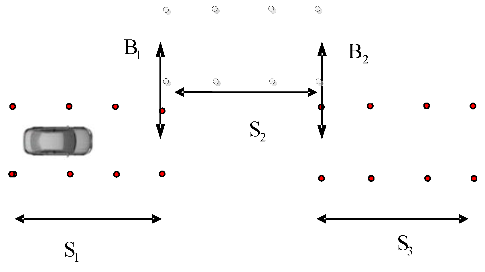
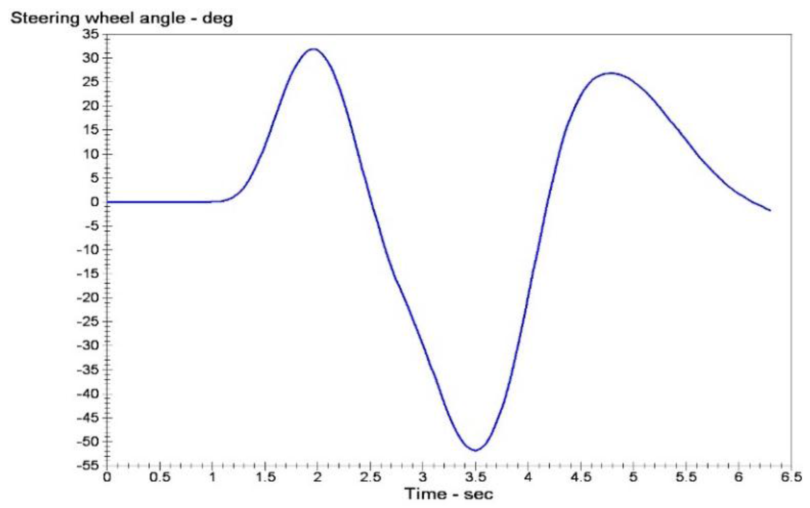
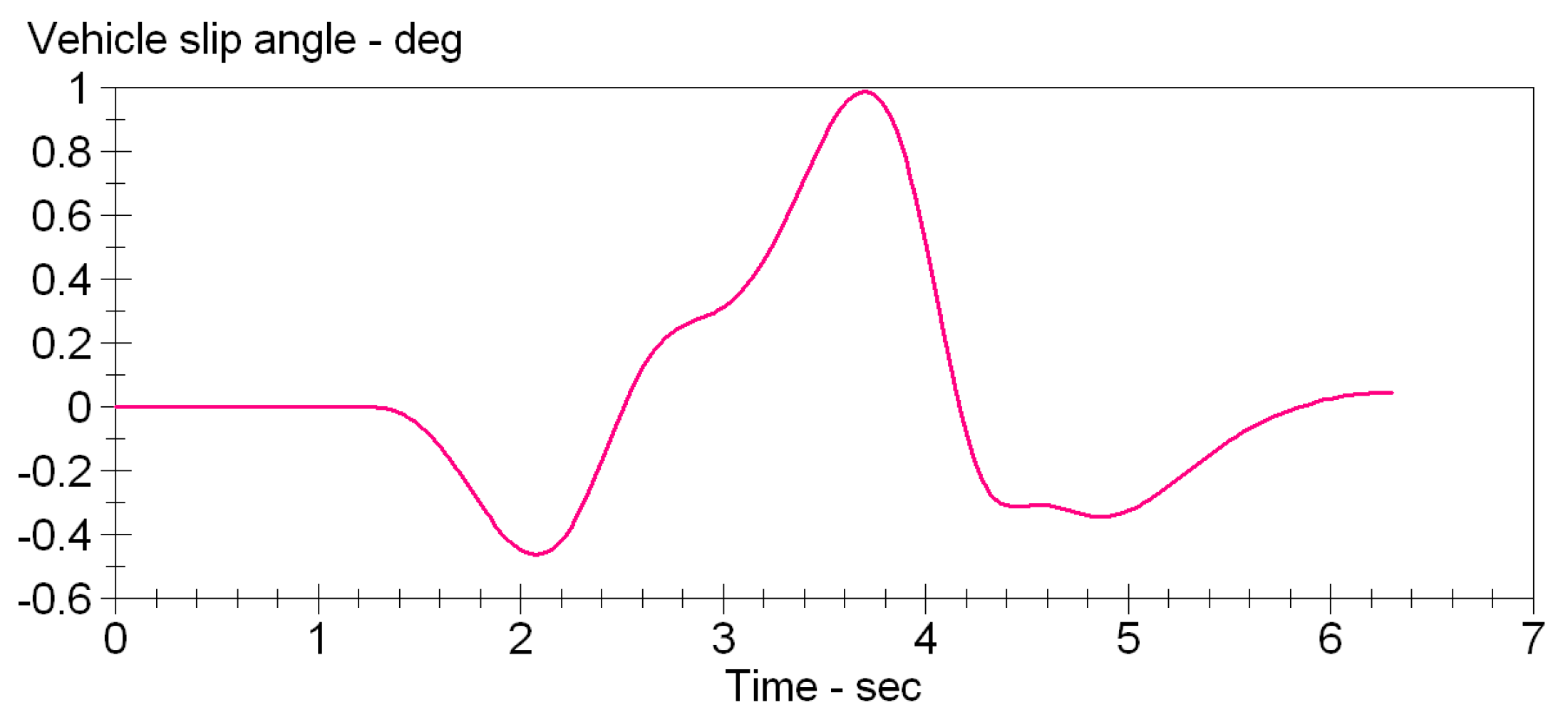
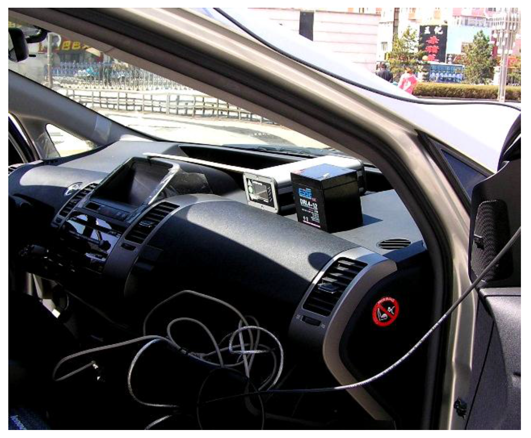
In this paper, an objective fuzzy interpolation before the Kalman algorithm is used for data synchronization. This objective fuzzy interpolation approach can work out time delays’ problem. Utilizing the integration of INS and GPS, fused by the two-stage Kalman filter, it can work out the problem of low update rate and GPS signal loss. The objective fuzzy interpolation method improves the accuracy effect of GPS/INS data fusion, and the two-stage Kalman filter is more robust. The RT3102 instrument is used to verify the effect of GPS/INS measurement and estimation of vehicle state parameters under typical driving conditions. The experimental consequences showed the approach of GPS and INS measurement for vehicle stability key parameters is accurate and robust.
4. Models of Vehicle Testing
4.1. Dynamical Model of Vehicle
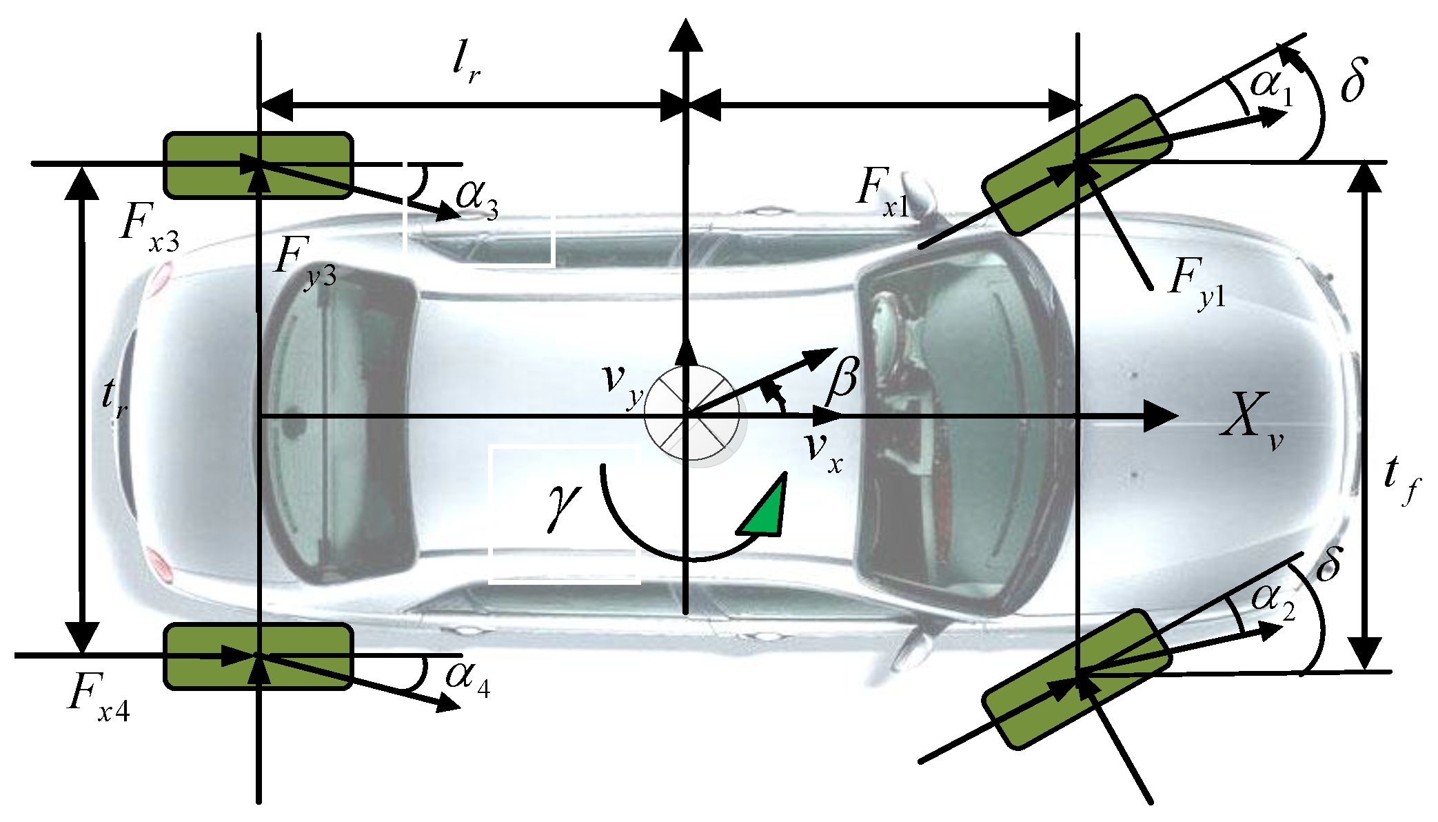
In order to reflect an automobile motion state, this paper establishes an eight degrees of freedom dynamic model including vehicle rotary motion, vehicle lateral motion, vehicle longitudinal motion, vehicle yaw motion, vehicle roll motion, four wheels rotary motion, steering wheel angle and vehicle speed. It is assumed that:
- (1)
Automobile vertical and pitch motions are ignored;
- (2)
The dynamic characteristics of the four tires are same;
- (3)
The influence of air resistance is ignored;
- (4)
The effect of sprung mass is ignored [
37].
According to
Figure 4, eight degrees of freedom dynamic equations are presented as the following:
Four wheels motion equation:
Figure 4.
Eight degrees of freedom (DOF) vehicle dynamic model.
Figure 4.
Eight degrees of freedom (DOF) vehicle dynamic model.
are wheels longitudinal resultant forces (). are wheels lateral resultant forces. is axis torque. m is vehicle mass. and are velocity components in and . and are distances between centroid to front and rear axles. and are distances between front and rear wheels. and are yaw velocity and yaw angular acceleration. is the moment of inertia around axle is the moment of inertia around . are the moments of inertia around and axle. are wheel angular velocity (). are wheel moments of inertia (). is wheel radius. are brake torque (). δ is steering wheel angle. are vehicle sprung mass. is the vertical distance from spring centroid to the roll center. is side angle. is the front suspension’s roll stiffness, and is the rear suspension’s roll stiffness. is the front suspension’s roll angle damping, and is the rear suspension’s roll angle damping.
4.2. Model of Two-Stage Kalman Filter
INS and GPS combination approaches consist of dynamic methods and kinematics methods. Kinematics approach is based on a vehicle’s movement relations, and it does not depend on estimating vehicle kinetics models. Since there is no modeling flaw, measure accurateness relies on the accurateness of the installation position and measuring apparatus, so this approach is very robust.
For the effect of discretization and time delays related to the GPS part, an important issue is the appropriate handing of the nonlinearities from uncertain time varying delays. In this work, an objective fuzzy interpolation before Kalman algorithm is used for data synchronization. This objective fuzzy interpolation method can solve the problem of time delays.
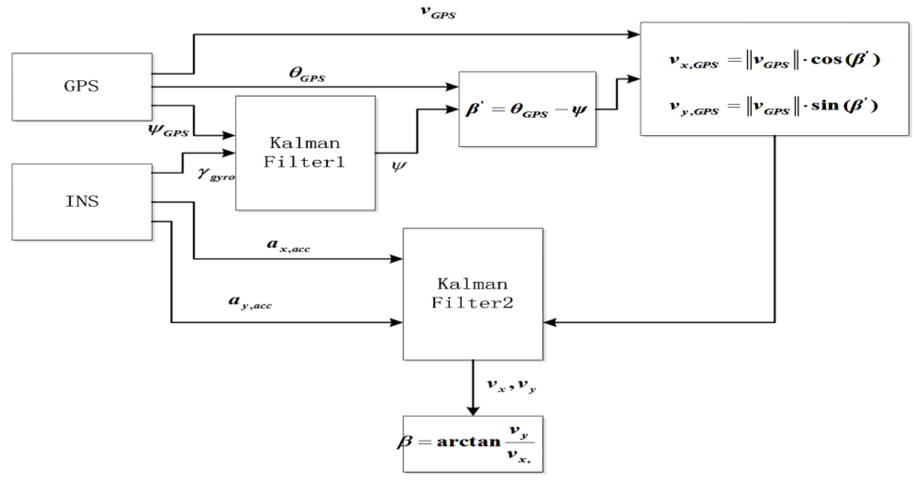
The fusion algorithm for vehicle sideslip angle that is based on the integration of GPS/INS was illustrated as
Figure 5. GPS measurement major values are azimuth angle
, speed
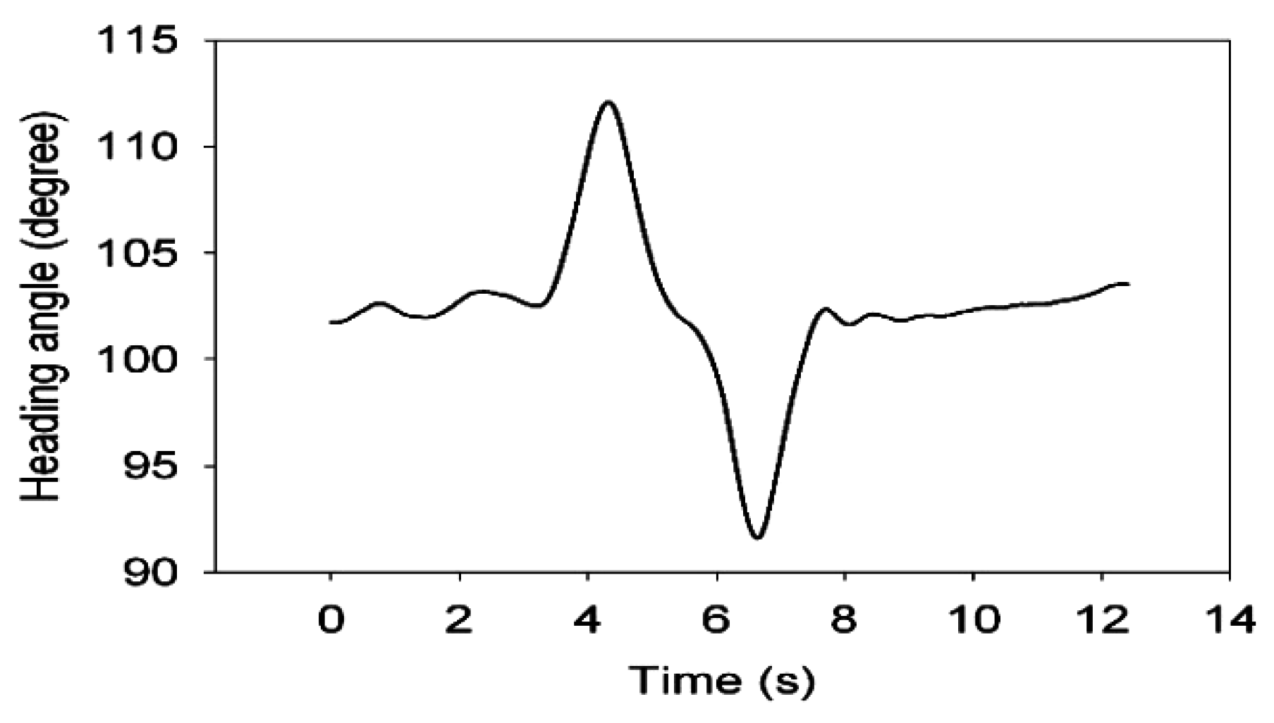
and heading angle
, and major values in INS measuring are longitudinal acceleration
, lateral acceleration
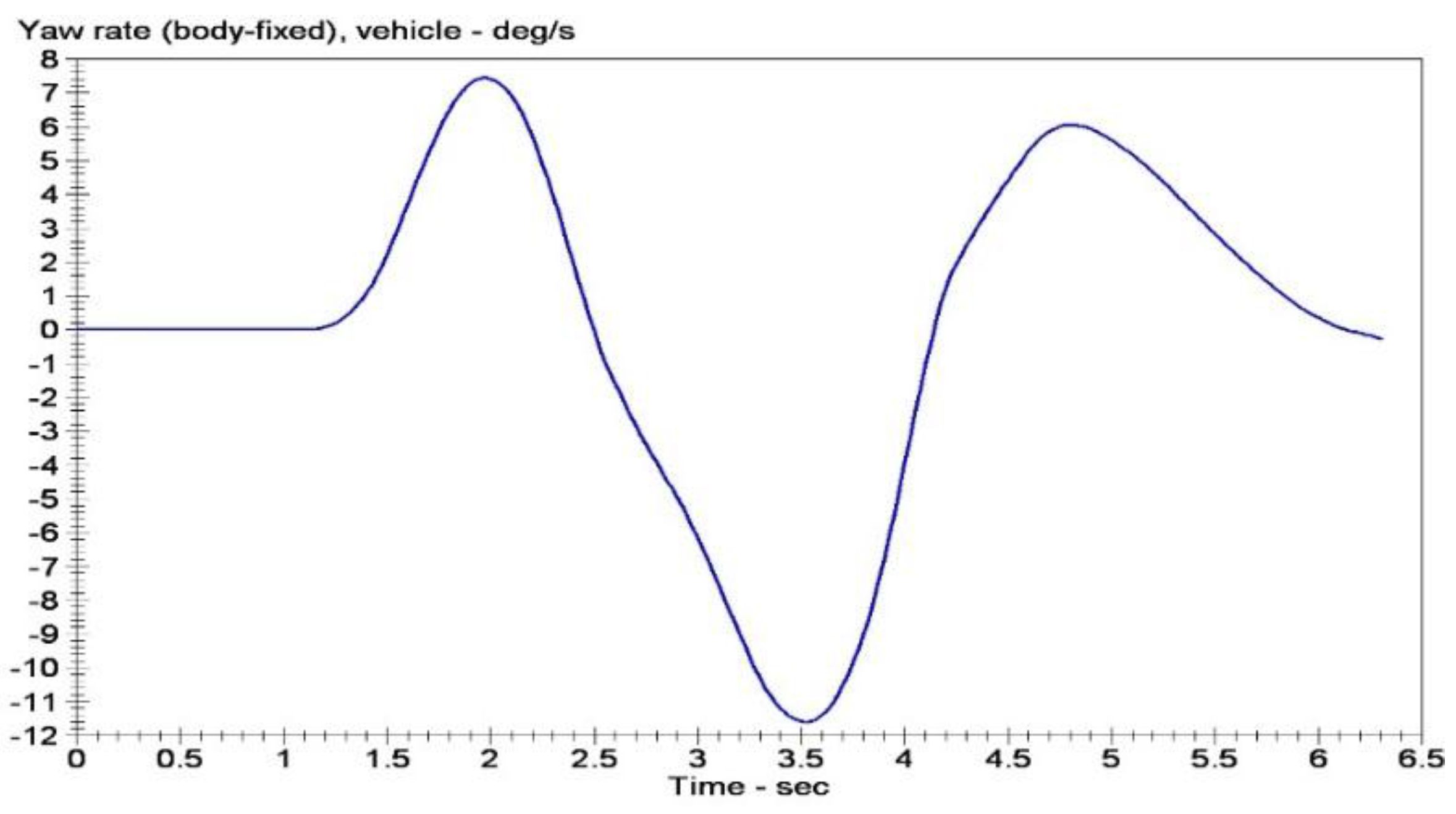
and yaw rate
.
Figure 5.
Sideslip angle two-stage Kalman filter block.
Figure 5.
Sideslip angle two-stage Kalman filter block.
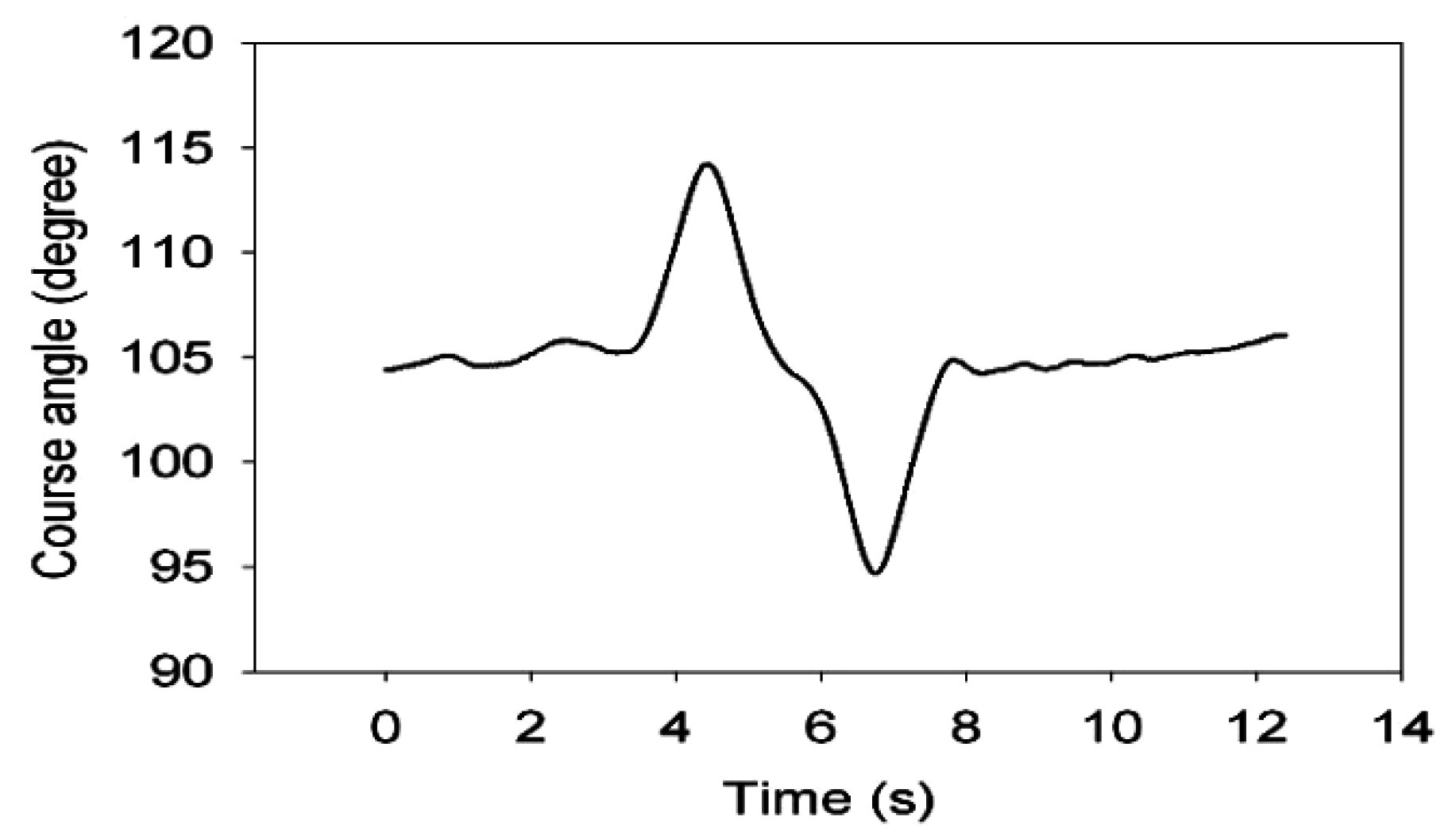
This work used two-stage Kalman filter to fuse GPS and INS measurement. First, yaw rate measured by gyro and heading angle measured by double antenna GPS receiver are fused by Kalman filter 1. The output is vehicle course angle . Longitudinal and lateral velocities are calculated according to the azimuth angle and velocity course angle . Second, the longitudinal and lateral acceleration measured by INS and the longitudinal and lateral velocities are fused by Kalman filter 2. The vehicle sideslip angle ratio can be obtained according to the vehicle sideslip angle .
Compared with the conventional GPS/INS algorithm, the algorithm has some advantages: Less state vector and computing times. Therefore, the algorithm can meet the requirement for real-time vehicle stability control. When GPS signal is lost, inertial navigation system can calculate the vehicle sideslip angle. At the same time, inertial navigation system achieves the error correction with GPS information.
4.3. Vehicle Stability Parameters Calculation
4.3.1. Vehicle Heading Angle Calculation
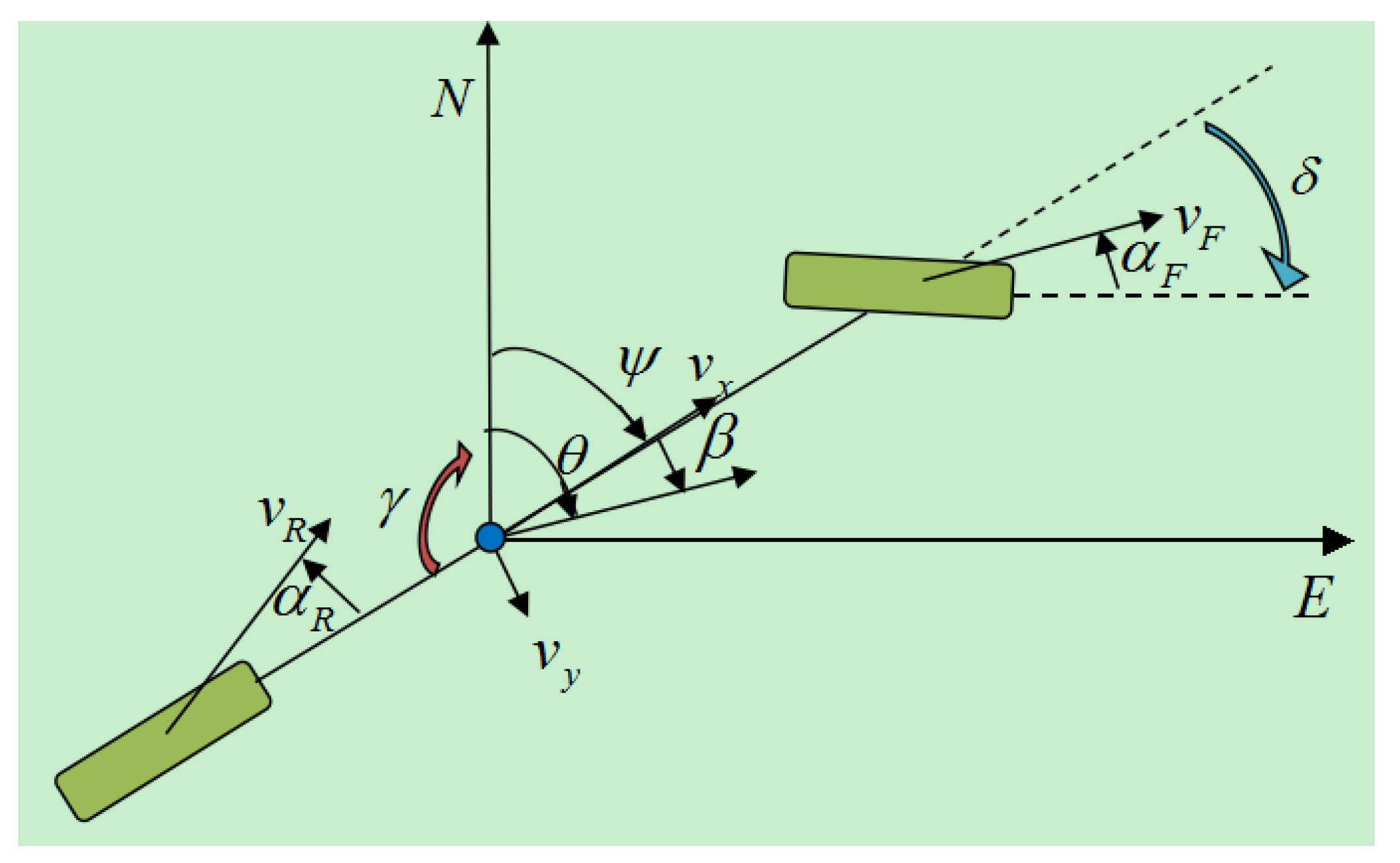
Yaw rate measured by gyro and heading angle measured by double antenna GPS receiver are fused by Kalman filter 1. In order to understand the heading, sideslip angles, azimuth and yaw and so forth,
Figure 6 shows the relationship between them.
Figure 6.
Illustrations of heading, yaw, azimuth and side slip angle.
Figure 6.
Illustrations of heading, yaw, azimuth and side slip angle.
Heading angle measured by dual antenna GPS receiver can be written as
is heading angle measured by GPS receiver. is GPS observation noise.
Yaw rate measured by gyroscope can be written as:
is yaw rate measured by gyroscopes. is heading angles. is yaw velocity deviation. is the gyro noise (the process noise).
The state equation of Kalman filter is written as the following:
Observation equation is written as:
The state vector x is , and the input is yaw rate measured by gyroscope. The observation value is the heading angle measured by GPS. If GPS is available, the observation matrix C is [1 0]. If GPS is not available, the observation matrix C is [0 0].
4.3.2. Vehicle Vertical and Horizontal Velocity Calculation
The longitudinal and lateral acceleration measured by INS and the longitudinal and lateral velocities are fused by Kalman filter 2.
(1) GPS measurement of the vehicle longitudinal and lateral velocity GPS measurement of the vehicle sideslip angle
is sideslip angle measured using INS and GPS. is the azimuth measured using GPS. is the heading angles measured by GPS and INS.
GPS measurement of the vehicle longitudinal and lateral velocity (vehicle body coordinate) can be written as:
If the main antenna of GPS is installed at the vehicle centroid, longitudinal and lateral velocity can be written as:
(2) Longitudinal and lateral velocity measured by acceleration sensor
is speed measured by GPS. and are longitudinal and lateral velocity components measured by GPS. and are longitudinal velocity and longitudinal acceleration measured through sensors. and are lateral velocity, lateral acceleration measured by sensors. and are lateral, longitudinal acceleration measured through acceleration sensors. and are lateral and longitudinal acceleration deviation. and are longitudinal and lateral GPS receiver noise. and are longitudinal and lateral acceleration sensor noise.
Kalman filter state equation:
where
Kalman filter observation equation:
is a state vector, and is observation values.
4.3.3. Vehicle Sideslip Angle Calculation
Sideslip angle measured by GPS and INS
When GPS signal is lost, no measurement can be done for , and . However, , and can be measured with an INS sensor. Then the sideslip angle can be determined.
The sideslip angle measured through GPS is the sideslip angle of GPS antenna. Usually the sideslip angle of vehicle centroid and even the wheel sideslip angle are needed. As the sideslip angle of GPS antenna is transformed into the sideslip angle of any point at vehicle, there should be a speed increment which angular velocity changes.
is the speed at P point. is the speed at main antenna of GPS. is the distance from main antenna to P. is yaw rate.
The sideslip angle of the point P is calculated by the following equation.
and is the velocity components in the vehicle body coordinates.


